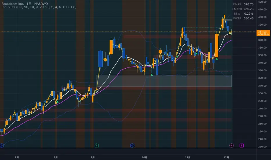
Ind-Suite: The Ultimate Strategic Dashboard [Gap/Dow/MA/SR]概要 Ind-Suiteは、トレードに必要な4つの重要な要素(窓、市場構造、移動平均線、水平線)を1つのインジケーターに統合した包括的なトレーディング・スイートです。 このツールの目的は、単一のサインに頼るのではなく、複数の根拠が重なる「コンフルエンス(Confluence)」を視覚的に発見することにあります。
機能モジュール 設定画面の「⚡ MODULE TOGGLES ⚡」から、各モジュールのON/OFFを瞬時に切り替えられます。
Module A: Gaps (窓)
未埋めの窓(Gap)をボックスで表示します。
価格が引き寄せられるターゲットとして機能します。一定期間経過した窓は自動的に非表示になります。
Module B: Dow Structure (ダウ理論と構造)
ZigZagラインによる波の描画と、トレンド状態の判定。
BOS (Break of Structure): トレンド継続のブレイクポイントにラベルを表示。
下落トレンド時は背景色が変化し、視覚的にトレンドを把握できます。
Module C: Safe Scaffold (足場と勢い)
EMA (9/20) & VWAP: トレンドフォローのための主要な移動平均線。
Bollinger Bands: ボラティリティの確認用(ON/OFF可能)。
Signal: EMAクロスとバンド幅拡大(スクイーズからのエクスパンション)を検知したロングサインを表示。
Module D: S/R Guardian (水平線)
過去のPivot点をベースに、意識されやすいサポート・レジスタンスラインを自動描画します。
強度に基づいてラインが統合され、重要度が高い価格帯を可視化します。
推奨される使い方 すべてのモジュールを常にONにする必要はありません。チャートが情報過多にならないよう、必要な機能だけを選択して表示してください。 例えば、「S/Rライン」での反発、「Dow Structure」でのBOS、「Gap」の埋め完了など、3つ以上の根拠が重なるポイントは、優位性の高いエントリーポイントとなります。
--------------
Overview Ind-Suite is a comprehensive trading suite that integrates four essential elements (Gaps, Market Structure, Moving Averages, and Support/Resistance) into a single indicator. The goal of this tool is not to rely on a single signal, but to visually identify "Confluence" where multiple factors align.
Feature Modules You can instantly toggle each module ON/OFF via the "⚡ MODULE TOGGLES ⚡" in the settings.
Module A: Gaps
Highlights unclosed gaps with boxes.
These act as price magnets/targets. Old gaps are automatically hidden after a set period.
Module B: Dow Structure (Trend & Market Structure)
Draws ZigZag waves and determines trend status based on pivot points.
BOS (Break of Structure): Labels are displayed at key breakout points confirming trend continuation.
Background color changes during downtrends for instant visual recognition.
Module C: Safe Scaffold (Momentum & MAs)
EMA (9/20) & VWAP: Key moving averages for trend following.
Bollinger Bands: For volatility analysis (Toggle available).
Signal: Displays Long signals upon EMA crossover combined with BBW expansion (volatility breakout).
Module D: S/R Guardian (Support & Resistance)
Automatically draws S/R zones based on historical pivot points.
Levels are merged based on proximity, visualizing significant price zones.
Recommended Usage It is not necessary to keep all modules ON at all times. Toggle features as needed to keep your chart clean. High-probability setups are often found where multiple factors converge (Confluence). For example: A bounce off an "S/R Line," confirmed by a "BOS" in Dow Structure, coinciding with a "Gap" fill.
Indicadores e estratégias
Self-Organized Criticality - Avalanche DistributionHere's all you need to know: This indicator applies Self-Organized Criticality (SOC) theory to financial markets, measuring the power-law exponent (alpha) of price drawdown distributions. It identifies whether markets are in stable Gaussian regimes or critical states where large cascading moves become more probable.
Self-Organized Criticality
SOC theory, introduced by Per Bak, Tang, and Wiesenfeld (1987), describes how complex systems naturally evolve toward critical (fragile) states. An example is a sand pile: adding grains creates avalanches whose sizes follow a power-law distribution rather than a normal distribution.
Financial markets exhibit similar behavior. Price movements aren't purely random walks—they display:
Fat-tailed distributions (more extreme events than Gaussian models predict)
Scale invariance (no characteristic avalanche size)
Intermittent dynamics (periods of calm punctuated by large cascades)
Power-Law Distributions
When a system is in a critical state, the probability of an avalanche of size s follows:
P(s) ∝ s^(-α)
Where:
α (alpha) is the power-law exponent
Higher α → distribution resembles Gaussian (large events rare)
Lower α → heavy tails dominate (large events common)
This indicator estimates α from the empirical distribution of price drawdowns.
Mathematical Method
1. Avalanche Detection
The indicator identifies local price peaks (highest point in a lookback window), then measures the percentage drawdown to the next trough. A dynamic ATR-based threshold filters out noise—small drops in calm markets count, but the bar rises in volatile periods.
2. Logarithmic Binning
Avalanche sizes are sorted into logarithmically-spaced bins (e.g., 1-2%, 2-4%, 4-8%) rather than linear bins. This captures power-law behavior across multiple scales - a 2% drop and 20% crash both matter. The indicator creates 12 adaptive bins spanning from your smallest to largest observed avalanche.
3. Bin-to-Bin Ratio Estimation
For each pair of adjacent bins, we calculate:
α ≈ log(N₁/N₂) / log(s₂/s₁)
Where N₁ and N₂ are avalanche counts, s₁ and s₂ are bin sizes.
Example: If 2% drops happen 4× more often than 4% drops, then α ≈ log(4)/log(2) ≈ 2.0.
We get 8-11 independent estimates and average them. This is more robust than fitting one line through all points—outliers can't dominate.
4. Rolling Window Analysis
Alpha recalculates using only recent avalanches (default: last 500 bars). Old data drops out as new avalanches occur, so the indicator tracks regime shifts in real-time.
Regime Classification
🟢 Gaussian α ≥ 2.8 Normal distribution behavior; large moves are rare outliers
🟡 Transitional 1.8 ≤ α < 2.8 Moderate fat tails; system approaching criticality
🟠 Critical 1.0 ≤ α < 1.8 Heavy tails; large avalanches increasingly common
🔴 Super-Critical α < 1.0 Extreme tail risk; system prone to cascading failures
What Alpha Tells You
Declining alpha → Market moving toward criticality; tail risk increasing
Rising alpha → Market stabilizing; returns to normal distribution
Persistent low alpha → Sustained fragility; heightened crash probability
Supporting Metrics
Heavy Tail %: Concentration of total drawdown in largest 10% of events
Populated Bins: Data coverage quality (11-12 out of 12 is ideal)
Avalanche Count: Sample size for statistical reliability
Limitations
This is a distributional measure, not a timing indicator. Low alpha indicates increased systemic risk but doesn't predict when a cascade will occur. Only that the probability distribution has shifted toward larger events.
How This Differs from the Per Bak Fragility Index
The SOC Avalanche Distribution calculates the power-law exponent (alpha) directly from price drawdown distributions - a pure mathematical analysis requiring only price data. The Per Bak Fragility Index aggregates external stress indicators (VIX, SKEW, credit spreads, put/call ratios) into a weighted composite score.
Technical Notes
Default settings optimized for daily and weekly timeframes on major indices
Requires minimum 200 bars of history for stable estimates
ATR-based dynamic sizing prevents scale-dependent bias
Alerts available for regime transitions and super-critical entry
References
Bak, P., Tang, C., & Wiesenfeld, K. (1987). Self-organized criticality: An explanation of the 1/f noise. Physical Review Letters.
Sornette, D. (2003). Why Stock Markets Crash: Critical Events in Complex Financial Systems. Princeton University Press.

50 EMA HLC Tejas50 EMA with All important sources. Made it with 50 EMA and Based on my understanding and observations.


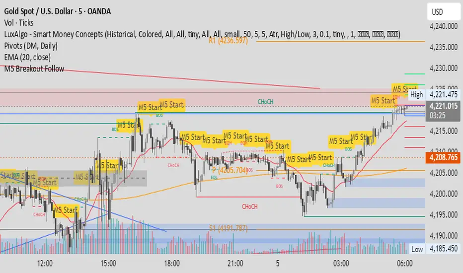
M5 Candle Follow Breakout - Teknik Gold Fanatic V2 This technique is entirely the property of Prof Sastra Gold Fanatic.
This technique uses a strategy of following breakouts from the first M5 of each hour.

Hull Moving Averages x 4Default Hull Lengths Included
The defaults are:
HMA 14
HMA 35
HMA 55
HMA 89
These are classic Fibonacci-style progression lengths, which work well for trend structure.

First Green/Red Week Day + Return SignalsWill give you the high of the first red day of the week and the low of the first green day of the week and gives you a signal when price returns and fails to breakout great signals

BigCandleAndRSIAlertChanges Candle Color to your choosing for Big Candles or Big Wick Candles or Over Bought/Oversold RSI Levels.

Jenkins OscillatorAn oscillator designed to capture price movement relative to recent intra-candle volatility. Z-score normalization is applied to smoothed price and therefore should be read in terms of standard deviation AND direction.


⚔️ The Scalpel⚔️ THE SCALPEL v2.0
━━━━━━━━━━━━━━━━━━━━━━━━━━━━━━━━━━━━━━━━━━━━━━━━━━━━━━━━
Surgical-Grade Market Structure Detection System
🔬 WHAT IS THE SCALPEL?
The Scalpel is a precision-engineered market structure analyzer that identifies and tracks critical support and resistance zones with surgical accuracy. Unlike conventional S&R tools that flood your chart with noise, The Scalpel cuts through the clutter to reveal only the most significant price structures.
━━━━━━━━━━━━━━━━━━━━━━━━━━━━━━━━━━━━━━━━━━━━━━━━━━━━━━━━
⚙️ CORE TECHNOLOGY
▸ Pivot-Based Detection Engine
Advanced pivot analysis calibrated by user-defined precision settings
▸ Tissue Integrity Validation
Filters structures based on candle body-to-range ratios
▸ Dynamic Stress Analysis
Tracks zone interactions and removes exhausted levels automatically
▸ Volatility-Adaptive Zones
Zone width scales with ATR for consistent performance across all markets
━━━━━━━━━━━━━━━━━━━━━━━━━━━━━━━━━━━━━━━━━━━━━━━━━━━━━━━━
🎨 VISUAL SPECTRUM
💜 STERILE ZONES (Electric Violet)
Fresh, untested structures with maximum potential
🔴 COMPRESSION ZONES (Magenta Fire)
Tested resistance ceilings under selling pressure
🩵 FOUNDATION ZONES (Neon Teal)
Tested support floors with proven buyer interest
✨ PLASMA AURA EFFECT
Multi-layered glow effect for enhanced visibility
━━━━━━━━━━━━━━━━━━━━━━━━━━━━━━━━━━━━━━━━━━━━━━━━━━━━━━━━
📐 PARAMETERS
🔪 Blade Precision (1-10)
Higher = fewer but sharper pivots detected
🩺 Tissue Integrity % (30-90)
Minimum candle body percentage required
📏 Incision Depth (0.1-2.0 ATR)
Controls zone thickness based on volatility
💉 Stress Threshold (1-10)
Maximum touches before zone invalidation
📐 Projection Range (10-200)
How far zones extend into the future
━━━━━━━━━━━━━━━━━━━━━━━━━━━━━━━━━━━━━━━━━━━━━━━━━━━━━━━━
💡 HOW TO USE
1. Fresh sterile zones (violet) are your highest-probability setups
2. Watch for price reaction at zone boundaries
3. Tested zones confirm structure but may have diminished strength
4. Zones auto-remove after stress threshold is reached
5. Use projection range to anticipate future tests
━━━━━━━━━━━━━━━━━━━━━━━━━━━━━━━━━━━━━━━━━━━━━━━━━━━━━━━━
🎯 BEST FOR
✓ Scalping & Day Trading
✓ Swing Trade Entries
✓ Stop Loss Placement
✓ Take Profit Targeting
✓ Multi-Timeframe Analysis
━━━━━━━━━━━━━━━━━━━━━━━━━━━━━━━━━━━━━━━━━━━━━━━━━━━━━━━━
⚠️ DISCLAIMER
This indicator is for educational purposes only. Always conduct your own analysis and use proper risk management. Past performance does not guarantee future results.
━━━━━━━━━━━━━━━━━━━━━━━━━━━━━━━━━━━━━━━━━━━━━━━━━━━━━━━━
🏷️ TAGS
support resistance zones SNR pivot points market structure scalping day trading swing trading price action order blocks smart money supply demand technical analysis

Ichimoku MTF HeatmapGreat for flying down you watchlist, getting an idea what time frame to go to. Enjoy!

Simulated Liquidation Heatmap [QuantAlgo]🟢 Overview
This indicator visualizes where clusters of stop-loss orders and liquidation levels are likely located, displayed as a 'heatmap'. It's based on the concept of market structure liquidity: large groups of stop orders tend to gather around obvious technical levels (like swing highs and lows), and these pools of orders often attract price movement from institutional traders. The indicator uses a fractal-based algorithm to identify these high-probability liquidation zones and displays them as dynamic, color-coded boxes.
The key feature is the thermal color gradient, which indicates the freshness (age) and therefore the relative relevance of the liquidity zone. Hot colors (e.g., Red/Yellow) represent fresh clusters that have just formed, suggesting strong and immediate liquidity interest. Cold colors (e.g., Blue/Purple) represent aged or decaying clusters that are becoming less relevant over time. This visualization allows traders to anticipate potential liquidity sweeps (stop hunts) and understand areas of significant retail and institutional positioning.
🟢 Key Features
1. Liquidity Zone Heatmap
The core function is the identification of swing high and swing low price points using a user-defined Lookback period. These points are where retail traders are statistically most likely to place their stop-loss orders. The indicator simulates the clustering of these orders by drawing a zone (box) around the detected swing point, with the vertical size controlled by the Stop/Liquidation Zone Width (%) setting.
▶ Cluster Lookback: Defines the sensitivity of swing point detection. Lower values detect frequent, minor zones (scalping/intraday); higher values detect major, stronger swing points (swing trading).
▶ Zone Width (%): Sets the percentage range above and below the swing point where stops are simulated to cluster, accounting for slippage and typical stop placement spread.
▶ Liquidity Decay: Zones gradually fade in color intensity and are eventually removed after the user-defined Liquidity Decay Period (Bars), ensuring the heatmap only displays relevant, current liquidity areas.
▶ Round Number Filter: An optional filter that limits the display to liquidity zones occurring only at psychologically significant round numbers (e.g., $100, $1,500.00), which typically attract higher concentrations of orders.
2. Thermal Color Gradient
The heatmap's color is a direct function of the zone's age, providing a visual proxy for immediate relevance.
▶ Freshness: Newly created zones are displayed in the Hot Color (high relevance).
▶ Decay: As bars pass, the zone color transitions along the gradient toward the Cold Color and increased transparency (lower relevance), until it is removed entirely.
▶ Color Schemes: Multiple pre-configured and custom color schemes are available to optimize the visualization for different chart themes and color preferences.
3. Liquidity Heat Thermometer
An optional visual thermometer is displayed on the chart to provide an instant, overall assessment of the current liquidation heat level in the immediate vicinity of the price.
▶ Calculation: The thermometer calculates an aggregate heat score based on the age and proximity of all liquidity zones within a user-defined Zone Detection Range (%) of the current price.
▶ Visual Feedback: A marker (triangle) points to the corresponding level on the thermometer's color gradient (Hot to Cold). A high reading indicates price is close to fresh, dense stop clusters, suggesting high volatility or an imminent liquidity sweep is probable. A low reading indicates price is in a low-density or aged liquidity area.
▶ Customization: The thermometer's resolution, position, and text size are fully customizable for optimal chart placement and readability.
🟢 Practical Applications
▶ Anticipate Sweeps: Prioritize trading in the direction of Hot (fresh) liquidity zones. For example, a hot low-side zone suggests strong sell-side liquidity (stop-losses) is available for large buyers to sweep.
▶ Filter Noise: Use the Round Number Filter to focus only on the highest probability liquidation zones, which are often at clean, psychological price levels.
▶ Validate Entries: Combine the Heat Thermometer with price action analysis. A rising heat level indicates increasing proximity to a major stop cluster, signaling a potential turn or an aggressive market move to sweep those stops.
▶ Risk Management: Understand that price often acts dynamically around these zones. High heat levels imply high risk/reward setups; stops should be placed strategically beyond the defined Liquidation Zone Width.
▶ Multi-Timeframe Context: Higher timeframes (e.g., Daily, 4-Hour) often reveal more significant, major liquidity zones. Use this indicator on lower timeframes (e.g., 5-min, 15-min) for execution, but prioritize zones that align with higher-timeframe structures.

X AVWAP DSOA powerful, non-overlay momentum indicator designed to measure the relationship between current price action and key Volume Weighted Average Price (VWAP) structures. It provides traders with a refined, configurable view of momentum by combining the **magnitude of price separation** with the **trend momentum** of the volume anchor.
---
### Core Calculation and Principle
This oscillator moves beyond simple price-vs-average separation by integrating the momentum (slope) of the volume average itself. The indicator is built around two primary components:
1. **Distance (D):** This is the magnitude of separation, calculated as the difference between the **closing price** and the selected **AVWAP Anchor Source** ($D = \text{Close} - \text{AVWAP}$).
2. **Slope (S):** This represents the **trend momentum** of the VWAP, calculated as the change in the smoothed AVWAP over a defined lookback period.
The final oscillator value is determined by the selected **Combination Method**, giving the user control over how these two factors interact:
* **Addition (Baseline):** The oscillator value is $D + S$. This provides a balanced view where the price separation is slightly adjusted by the VWAP's momentum.
* **Weighted Addition:** The oscillator value is $D + (S \times \text{Weight})$. This is a powerful feature that **allows the user to prioritize the impact of the Slope (trend momentum) over the Distance (magnitude)** using a customizable multiplier called the **Slope Weight**.
---
### Customization and Flexibility
The indicator's value lies in its deep configurability, allowing it to adapt to different trading strategies and timeframes:
* **AVWAP Anchor Source:** You can toggle between two critical VWAP reset structures for context:
* **4H Session VWAP:** Uses fixed, sequential 4-hour VWAP segments (e.g., 18:00, 22:00 NY Time) for tracking short-term structural shifts.
* **Daily AVWAP (ETH 18:00):** Uses a single, continuous VWAP anchored from the Electronic Trading Hours (ETH) open at 18:00 NY Time, providing a broader, sustained volume-weighted average context.
* **VWAP Price Source:** The underlying price used to calculate the VWAP itself is selectable (options include Close, OHLC4, HLC3, Open, High, and Low).
* **Plot Style:** Toggle between a continuous **Line** plot (for tracking fine movements) and a color-coded **Histogram** (for clear magnitude and directional reading, with Blue for positive and Red for negative).
### Trading Application
The AVWAP Distance & Slope Oscillator is a sophisticated tool best used to identify:
* **Zero-Line Crosses:** Signifying price crossing the underlying volume anchor while accounting for the anchor's own momentum.
* **Momentum Confirmation:** A high positive reading indicates price is strongly above the VWAP, and the VWAP itself is actively rising (strong bullish momentum).
* **Filtered Signals:** By adjusting the **Slope Weight** (in the Weighted Addition method), traders can amplify signals when the structural trend (VWAP slope) is strong, helping to filter out minor price fluctuations that occur when the VWAP is relatively flat.


Angular Resistance & Breakout/BreakdownAngular Resistance & Breakout/Breakdown (Dynamic Trendlines)
This indicator provides a dynamic approach to identifying major support and resistance levels by fitting Linear Regression lines to recent pivot points (swing highs and swing lows). Unlike static horizontal lines, these "Angular" trendlines adapt to the market's slope, providing continuously adjusting targets for resistance and support, along with signals for confirmed breakouts and breakdowns.
💡 Key Features
Dynamic Trendlines: Utilizes Linear Regression to automatically draw sloped trendlines based on a configurable number of the most recent swing pivots.
Confirmed Signals: Generates clear Breakout (▲) and Breakdown (▼) signals with optional buffer and sensitivity filters to reduce noise.
Customizable Inputs: Fine-tune the pivot detection period, the number of points used for regression, line extension, and signal sensitivity.
On-Chart Info Panel: A table displays real-time data, including the number of detected pivot points and the current calculated price level of the dynamic lines.
⚙️ How It Works (The Logic)
Pivot Detection: The script uses the standard ta.pivothigh() and ta.pivotlow() functions to reliably identify swing points, based on the Pivot Left and Pivot Right settings. These points are stored in dynamic arrays (highs for resistance, lows for support).
Angular Line Generation: A custom function, f_regression_from_array, performs a Linear Regression analysis using the bar index (X-axis) and the pivot price (Y-axis) for the Points to use. This calculation determines the optimal slope and intercept to draw a best-fit dynamic line through the identified pivot points.
Breakout/Breakdown Confirmation:
Breakout: Triggered when the current close price crosses above the dynamic resistance line plus the user-defined Breakout buffer.
Breakdown: Triggered when the current close price crosses below the dynamic support line minus the user-defined Breakout buffer.
Sensitivity Filter: An optional filter requires the price movement on the signal bar to exceed a minimum percentage (Label sensitivity) away from the line to confirm the momentum of the move.

Ichimoku Traffic Lights Go--no go flags for Ichimoku Cloud. For quick scanning thru your watchlist, and good for scanning through timeframes.

CANDLE_TIME_RDThis tool displays the time of each candle directly on the chart by placing a label below
the bar with an upward-pointing arrow for clear visual alignment. It helps traders quickly
identify the exact timestamp of any candle during fast intraday analysis or historical review.
OVERVIEW
The script extracts the hour and minute of each bar, formats the timestamp according to the
user’s preference, and prints it beneath the candle. This removes the need to rely on the
data window or crosshair for time inspection. It is ideal for ITI evaluation, timestamp
journaling, and precise replay study.
FEATURES
- Prints the time under each candle or every N-th candle using a simple step input.
- Supports both AM/PM and military time through a toggle input.
- Builds all hour and minute text manually to ensure consistent formatting.
- Uses label.style_label_up to draw an arrow pointing toward the candle.
- Positions labels with yloc.belowbar so they do not overlap price bars.
USE CASES
- Reviewing setups with ChatGPT where exact candle timing matters.
- Studying EMA touches, VWAP interactions, or momentum shifts that occur at specific times.
- Journaling entries and exits with precise timestamps.
- Quickly identifying candle times without zooming or opening data windows.
This script is designed for clarity and convenience, improving workflow for structured
intraday traders and replay analysts.

TWAP High LowTWAP that anchors from the daily high and low, day starting at the settlement period, 14:59:30CT

Weeknights Guppy Trend Strength OscillatorBuilt a Guppy Oscillator which takes 22 different EMA's and uses an ATR to provide slope normalisation. The goal is to help the user determine strength of trend and see if momentum is slowing
On its own I doubt it will provide a full trading system but I believe it can help provide confluence to ones trading decisions
Left it open source

TWAP OscillatorIts an oscillator for the daily TWAP, anchored from 14:59:30CT which is the settlement time for the SP500 and Emini500. There are 5 deviations ranges for the oscillator matching the 5 deviations from the other Daily TWAP script. The RSI colors the line, I stole the RSI coloring from ChartPrime, thanks.
