EMA Envelope + SMA + Purple DotThis indicator combines three tools into one:
📈 EMA Envelope with wedge and range contraction signals to highlight volatility squeezes.
🔵 SMA with optional smoothing (SMA/EMA/WMA/SMMA/VWMA) and optional Bollinger Bands.
🟣 Purple Dot “PowerBars” that mark strong momentum bars when price ROC (%) and volume exceed user-defined thresholds.
It also includes:
Background highlighting of contraction zones (bullish/bearish/neutral colors).
A summary table showing PowerBar count and return (%) over custom lookback periods.
Flexible display settings (table position, dark/light theme, highlight toggle).
Designed for traders who want to track momentum bursts, volatility contraction, and trend strength all in one tool.
Volatilidade

Theil-Sen Line Filter [BackQuant]Theil-Sen Line Filter
A robust, median-slope baseline that tracks price while resisting outliers. Designed for the chart pane as a clean, adaptive reference line with optional candle coloring and slope-flip alerts.
What this is
A trend filter that estimates the underlying slope of price using a Theil-Sen style median of past slopes, then advances a baseline by a controlled fraction of that slope each bar. The result is a smooth line that reacts to real directional change while staying calm through noise, gaps, and single-bar shocks.
Why Theil-Sen
Classical moving averages are sensitive to outliers and shape changes. Ordinary least squares is sensitive to large residuals. The Theil-Sen idea replaces a single fragile estimate with the median of many simple slopes, which is statistically robust and less influenced by a few extreme bars. That makes the baseline steadier in choppy conditions and cleaner around regime turns.
What it plots
Filtered baseline that advances by a fraction of the robust slope each bar.
Optional candle coloring by baseline slope sign for quick trend read.
Alerts when the baseline slope turns up or down.
How it behaves (high level)
Looks back over a fixed window and forms many “current vs past” bar-to-bar slopes.
Takes the median of those slopes to get a robust estimate for the bar.
Optionally caps the magnitude of that per-bar slope so a single volatile bar cannot yank the line.
Moves the baseline forward by a user-controlled fraction of the estimated slope. Lower fractions are smoother. Higher fractions are more responsive.
Inputs and what they do
Price Source — the series the filter tracks. Typical is close; HL2 or HLC3 can be smoother.
Window Length — how many bars to consider for slopes. Larger windows are steadier and slower. Smaller windows are quicker and noisier.
Response — fraction of the estimated slope applied each bar. 1.00 follows the robust slope closely; values below 1.00 dampen moves.
Slope Cap Mode — optional guardrail on each bar’s slope:
None — no cap.
ATR — cap scales with recent true range.
Percent — cap scales with price level.
Points — fixed absolute cap in price points.
ATR Length / Mult, Cap Percent, Cap Points — tune the chosen cap mode’s size.
UI Settings — show or hide the line, paint candles by slope, choose long and short colors.
How to read it
Up-slope baseline and green candles indicate a rising robust trend. Pullbacks that do not flip the slope often resolve in trend direction.
Down-slope baseline and red candles indicate a falling robust trend. Bounces against the slope are lower-probability until proven otherwise.
Flat or frequent flips suggest a range. Increase window length or decrease response if you want fewer whipsaws in sideways markets.
Use cases
Bias filter — only take longs when slope is up, shorts when slope is down. It is a simple way to gate faster setups.
Stop or trail reference — use the line as a trailing guide. If price closes beyond the line and the slope flips, consider reducing exposure.
Regime detector — widen the window on higher timeframes to define major up vs down regimes for asset rotation or risk toggles.
Noise control — enable a cap mode in very volatile symbols to retain the line’s continuity through event bars.
Tuning guidance
Quick swing trading — shorter window, higher response, optionally add a percent cap to keep it stable on large moves.
Position trading — longer window, moderate response. ATR cap tends to scale well across cycles.
Low-liquidity or gappy charts — prefer longer window and a points or ATR cap. That reduces jumpiness around discontinuities.
Alerts included
Theil-Sen Up Slope — baseline’s one-bar change crosses above zero.
Theil-Sen Down Slope — baseline’s one-bar change crosses below zero.
Strengths
Robust to outliers through median-based slope estimation.
Continuously advances with price rather than re-anchoring, which reduces lag at turns.
User-selectable slope caps to tame shock bars without over-smoothing everything.
Minimal visuals with optional candle painting for fast regime recognition.
Notes
This is a filter, not a trading system. It does not account for execution, spreads, or gaps. Pair it with entry logic, risk management, and higher-timeframe context if you plan to use it for decisions.

Ark FCI OscillatorFinancial Conditions Index Oscillator
This indicator tracks week-over-week changes in the National Financial Conditions Index (NFCI), providing a dynamic view of evolving financial conditions in the United States.
Overview
The National Financial Conditions Index (NFCI) is a comprehensive weekly composite index published by the Federal Reserve Bank of Chicago. It measures financial conditions across U.S. money markets, debt and equity markets, and the traditional and shadow banking systems.
Interpretation
Positive values indicate improving financial conditions
Negative values signal deteriorating financial conditions
Risk assets demonstrate particular sensitivity to changes in financial conditions, making this oscillator valuable for market timing and risk assessment.
Alternative Data Source
Users can modify the source to FRED:NFCIRISK to focus specifically on risk dynamics. The NFCIRISK subindex isolates volatility and funding risk measures within the financial sector, capturing market volatility indicators and liquidity shortage probabilities while excluding broader credit and leverage conditions.

Volume + RSI & MA Differential"Volume + RSI & MA Differential," integrates volume, RSI, and moving average differentials to generate trading signals. The script calculates a 14-period RSI to identify overbought or oversold conditions, with customizable thresholds for buy and sell signals. It also computes a 20-period SMA of the volume to smooth out trading activity data, helping to identify trends in market participation.
The script incorporates a fast (50-period) and a slow (200-period) SMA to analyze short-term and long-term trends, respectively. The differential between these moving averages, adjusted by the volume SMA, is used to identify potential trend changes or confirmations. Bars are colored yellow when the RSI is below the buy threshold and volume is high, indicating a potential buy signal. Conversely, bars turn red when the RSI is above the sell threshold and the fast MA is below the current close price, suggesting a potential sell signal. Neutral conditions result in grey bars.
Additionally, the script uses color-coding to plot the volume SMA and a line that changes color based on the moving average differential. A black line indicates a broadening MA cloud and a bullish trend, while a grey line suggests a narrowing MA cloud and a potential selloff. A yellow line signals the beginning of a buyback. This visual representation helps traders quickly identify potential trading opportunities and trend changes, making the script a valuable tool for technical analysis.
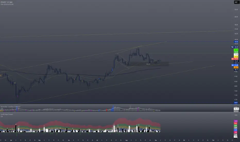
Candle Spread + ATR SMA Analysis
This indicator combines elements from two popular open-source scripts — Candle Range Compare
by @oldinvestor
and Objective Analysis of Spread (VSA)
by @Rin-Nin
— into a single tool for analyzing candle spreads (ranges and bodies) in relation to volatility benchmarks.
🔎 What It Does
Candle Decomposition:
Plots total candle ranges (high–low) in gray, for both up and down closes.
Plots up-close bodies (open–close) in white.
Plots down-close bodies in black.
This makes it easy to spot whether volatility comes from real price movement (body) or extended wicks.
ATR & SMA Volatility Bands:
Calculates ATR (Average True Range) and overlays it as a black line.
Plots four volatility envelopes derived from the SMA of the true range:
0.8× (blue, shaded)
1.3× (green)
1.8× (red)
3.0× (purple)
Colored fill zones highlight when candle spreads are below, within, or above key thresholds.
Visual Context:
Track expansion/contraction in spreads.
Compare bullish (white) vs bearish (black) bodies to gauge buying/selling pressure.
Identify when candles stretch beyond typical volatility ranges.
📈 How To Use It
VSA context: Wide down bars (black) beyond ATR bands may suggest supply; wide up bars (white) may indicate demand.
Trend confirmation: Expanding ranges above average thresholds (green/red/purple bands) often confirm momentum.
Reversal potential: Small bodies but large ranges (gray + wicks) frequently appear at turning points.
Volatility filter: Use ATR bands to filter trades — e.g., only act when candle ranges exceed 1.3× or 1.8× SMA thresholds.
🙏 Credits
This script is inspired by and combines ideas from:
Candle Range Compare
by @oldinvestor
Objective Analysis of Spread (VSA)
by @Rin-Nin
Big thanks to both authors for their valuable contributions to the TradingView community.
One thing I couldnt quite get to work is being able to display up and down wicks like in the candle range compare, so I just add that indicator to the chart as well, uncheck everything but the wick plots and there it is.
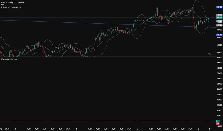
PCV (Darren.L-V2)Description:
This indicator combines Bollinger Bands, CCI, and RVI to help identify high-probability zones on M15 charts.
Features:
Bollinger Bands (BB) – displayed on the main chart in light gray. Helps visualize overbought and oversold price levels.
CCI ±100 levels + RVI – displayed in a separate sub-window:
CCI only shows the ±100 reference lines.
RVI displays a cyan main line and a red signal line.
Valid Zone Detection:
Candle closes outside the Bollinger Bands.
RVI crosses above +100 or below -100 (CCI level reference).
Candle closes back inside the BB, confirming a price rebound.
Requires two touches in the same direction to confirm the zone.
Only zones within 20–30 pips range are considered valid.
Usage:
Helps traders spot reversal or bounce zones with clear visual signals.
Suitable for all indices, Forex, and crypto on M15 timeframe.
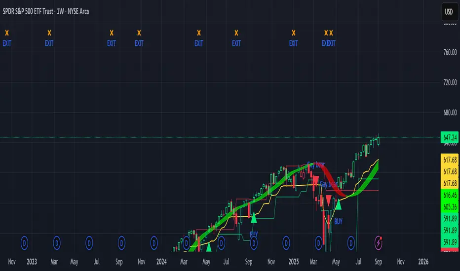
Sniper Swing — Short TF (Clean Signals) [v6]📘 How to Use the Sniper Swing Indicator
1. What It Does
It looks for short-term swing breaks in price.
It uses an oscillator (RSI/Stoch) and swing pivots to confirm moves.
It gives you 3 clear signals only:
BUY → Enter long (expecting price to go up).
Gay bear → Enter short (expecting price to go down).
EXIT → Close your trade (long or short).
Candles also change color:
Green = in a BUY trade.
Red = in a Gay bear trade.
Neutral (gray/none) = no trade.
2. When to Use
Works best on short timeframes (1m–5m) for scalping/intraday.
Use on liquid markets (MES/ES, NQ, SPY, BTC, ETH).
Avoid dead hours with no volume (like overnight futures lull or midday chop).
3. How to Trade With It
A. BUY trade
Wait for a BUY triangle below the candle.
Confirm:
Candle turned green.
Price broke a recent swing high.
Oscillator shows strength (indicator does this for you).
Enter long at the close of that candle.
Place your stop-loss:
At the yellow stop line (auto trailing stop), or
Just below the last swing low.
Stay in while candles are green.
Exit when:
An orange X appears, or
Price hits your stop.
B. Gay bear (short) trade
Wait for a Gay bear triangle above the candle.
Confirm:
Candle turned red.
Price broke a recent swing low.
Oscillator shows weakness.
Enter short at the close of that candle.
Place stop-loss:
At the yellow stop line, or
Just above the last swing high.
Stay in while candles are red.
Exit on an orange X or stop hit.
4. Pro Tips for New Traders
Only take one signal at a time → don’t double dip.
Quality > Quantity: ignore weak, sideways markets. Best signals happen during trends.
Start small: trade micros (MES) or small position sizes.
Use alerts: set TradingView alerts for BUY/Gay bear/EXIT so you don’t miss setups.
Think of the indicator like a navigator: it tells you the likely path, but you’re the driver → always manage risk.
5. Quick Mental Checklist
Signal? (BUY or Gay bear triangle)
Confirmed? (candle color + swing break)
Enter? (on close)
Stop? (yellow line or swing)
Exit? (orange X or stop)
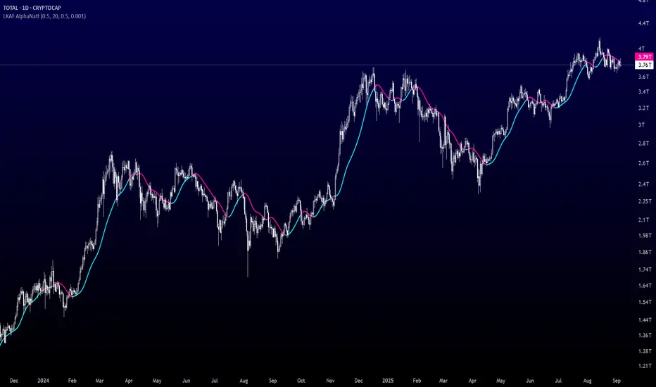
Laguerre-Kalman Adaptive Filter | AlphaNattLaguerre-Kalman Adaptive Filter |AlphaNatt
A sophisticated trend-following indicator that combines Laguerre polynomial filtering with Kalman optimal estimation to create an ultra-smooth, low-lag trend line with exceptional noise reduction capabilities.
"The perfect trend line adapts to market conditions while filtering out noise - this indicator achieves both through advanced mathematical techniques rarely seen in retail trading."
━━━━━━━━━━━━━━━━━━━━━━━━━━━━━━━━━━━━━━━━
🎯 KEY FEATURES
Dual-Filter Architecture: Combines two powerful filtering methods for superior performance
Adaptive Volatility Adjustment: Automatically adapts to market conditions
Minimal Lag: Laguerre polynomials provide faster response than traditional moving averages
Optimal Noise Reduction: Kalman filtering removes market noise while preserving trend
Clean Visual Design: Color-coded trend visualization (cyan/pink)
━━━━━━━━━━━━━━━━━━━━━━━━━━━━━━━━━━━━━━━━
📊 THE MATHEMATICS
1. Laguerre Filter Component
The Laguerre filter uses a cascade of four all-pass filters with a single gamma parameter:
4th order IIR (Infinite Impulse Response) filter
Single parameter (gamma) controls all filter characteristics
Provides smoother output than EMA with similar lag
Based on Laguerre polynomials from quantum mechanics
2. Kalman Filter Component
Implements a simplified Kalman filter for optimal estimation:
Prediction-correction algorithm from aerospace engineering
Dynamically adjusts based on estimation error
Provides mathematically optimal estimate of true price trend
Reduces noise while maintaining responsiveness
3. Adaptive Mechanism
Monitors market volatility in real-time
Adjusts filter parameters based on current conditions
More responsive in trending markets
More stable in ranging markets
━━━━━━━━━━━━━━━━━━━━━━━━━━━━━━━━━━━━━━━━
⚙️ INDICATOR SETTINGS
Laguerre Gamma (0.1-0.99): Controls filter smoothness. Higher = smoother but more lag
Adaptive Period (5-100): Lookback for volatility calculation
Kalman Noise Reduction (0.1-2.0): Higher = more noise filtering
Trend Threshold (0.0001-0.01): Minimum change to register trend shift
Recommended Settings:
Scalping: Gamma: 0.6, Period: 10, Noise: 0.3
Day Trading: Gamma: 0.8, Period: 20, Noise: 0.5 (default)
Swing Trading: Gamma: 0.9, Period: 30, Noise: 0.8
Position Trading: Gamma: 0.95, Period: 50, Noise: 1.2
━━━━━━━━━━━━━━━━━━━━━━━━━━━━━━━━━━━━━━━━
📈 TRADING SIGNALS
Primary Signals:
Cyan Line: Bullish trend - price above filter and filter ascending
Pink Line: Bearish trend - price below filter or filter descending
Color Change: Potential trend reversal point
Entry Strategies:
Trend Continuation: Enter on pullback to filter line in trending market
Trend Reversal: Enter on color change with volume confirmation
Breakout: Enter when price crosses filter with momentum
Exit Strategies:
Exit long when line turns from cyan to pink
Exit short when line turns from pink to cyan
Use filter as trailing stop in strong trends
━━━━━━━━━━━━━━━━━━━━━━━━━━━━━━━━━━━━━━━━
✨ ADVANTAGES OVER TRADITIONAL INDICATORS
Vs. Moving Averages:
Significantly less lag while maintaining smoothness
Adaptive to market conditions
Better noise filtering
Vs. Standard Filters:
Dual-filter approach provides optimal estimation
Mathematical foundation from signal processing
Self-adjusting parameters
Vs. Other Trend Indicators:
Cleaner signals with fewer whipsaws
Works across all timeframes
No repainting or lookahead bias
━━━━━━━━━━━━━━━━━━━━━━━━━━━━━━━━━━━━━━━━
🎓 MATHEMATICAL BACKGROUND
The Laguerre filter was developed by John Ehlers, applying Laguerre polynomials (used in quantum mechanics) to financial markets. These polynomials provide an elegant solution to the lag-smoothness tradeoff that plagues traditional moving averages.
The Kalman filter, developed by Rudolf Kalman in 1960, is used in everything from GPS systems to spacecraft navigation. It provides the mathematically optimal estimate of a system's state given noisy measurements.
By combining these two approaches, this indicator achieves what neither can alone: a smooth, responsive trend line that adapts to market conditions while filtering out noise.
━━━━━━━━━━━━━━━━━━━━━━━━━━━━━━━━━━━━━━━━
💡 TIPS FOR BEST RESULTS
Confirm with Volume: Strong trends should have increasing volume
Multiple Timeframes: Use higher timeframe for trend, lower for entry
Combine with Momentum: RSI or MACD can confirm filter signals
Market Conditions: Adjust noise parameter based on market volatility
Backtesting: Always test settings on your specific instrument
━━━━━━━━━━━━━━━━━━━━━━━━━━━━━━━━━━━━━━━━
⚠️ IMPORTANT NOTES
No indicator is perfect - always use proper risk management
Best suited for trending markets
May produce false signals in choppy/ranging conditions
Not financial advice - for educational purposes only
━━━━━━━━━━━━━━━━━━━━━━━━━━━━━━━━━━━━━━━━
🚀 CONCLUSION
The Laguerre-Kalman Adaptive Filter represents a significant advancement in technical analysis, bringing institutional-grade mathematical techniques to retail traders. Its unique combination of polynomial filtering and optimal estimation provides a clean, reliable trend-following tool that adapts to changing market conditions.
Whether you're scalping on the 1-minute chart or position trading on the daily, this indicator provides clear, actionable signals with minimal false positives.
"In the world of technical analysis, the edge comes from using better mathematics. This indicator delivers that edge."
━━━━━━━━━━━━━━━━━━━━━━━━━━━━━━━━━━━━━━━━
Developed by AlphaNatt | Professional Quantitative Trading Tools
Version: 1.0
Last Updated: 2025
Pine Script: v6
License: Open Source
Not financial advice. Always DYOR
PumpC ATR Line LevelsPumpC ATR Line Levels
Overview
PumpC ATR Line Levels is a volatility-based indicator that projects potential expansion levels from the previous session’s close using the Average True Range (ATR). This tool builds upon the Previous OHLC framework created by Nephew_Sam_ by extending its session-handling logic and adding ATR-based levels, statistical tracking, and flexible visualization options.
How It Works
Calculates ATR from a user-selectable higher timeframe (default: Daily).
Projects levels above and below the previous session’s close (or current close when preview mode is enabled).
Supports up to 5 ATR multiples, each with independent toggles, colors, and labels.
Optionally displays only the most recent ATR session for clarity.
Includes a data table tracking how often ATR levels are reached or closed beyond.
Features
Configurable ATR timeframe and length (default: 21).
Default multiples: 0.30, 0.60, 0.90; optional: 1.236, 2.00.
Toggle for preview mode (using current close vs. locked prior session close).
Customizable line style, width, colors, and label placement.
Visibility filter to show only on chart TF ≤ 60 minutes.
Session statistics table with counts and percentages of level interactions.
Use Cases
Identify intraday expansion targets or stop placement zones based on volatility.
Evaluate historical tendencies of price respecting or breaking ATR bands.
Support volatility-adjusted trade planning with statistical validation.
Acknowledgment
This script was developed on top of the Previous OHLC indicator by Nephew_Sam_ , with major modifications to implement ATR-driven levels, extended statistics, and customizable table output.
Notes
This indicator does not generate buy/sell signals.
Best applied to intraday charts anchored to a higher-timeframe ATR.
Keep charts clean and avoid non-standard bar types when publishing.

BTC Sigma CloudOverview
The BTC Sigma Cloud indicator calculates and displays 1, 2, and 3 sigma price movements for Bitcoin (BTC) on a rolling basis, visualized as a cloud. It shows historical volatility bands and projects them forward for the next 7 days.
Settings:
Vol Lookback: Default is 20 periods. Adjust to change the volatility calculation window.
Interpretation:
Cloud Bands: The cloud consists of three shaded layers representing 1σ, 2σ, and 3σ moves above and below the current price.
1σ (Innermost): 68% probability of price staying within this range.
2σ (Middle): 95% probability.
3σ (Outermost): 99.7% probability.
Historical View: The cloud tracks past price movements based on volatility.
Projection: The cloud extends 7 days forward, indicating potential price ranges based on current volatility.
Labels: Subtle labels (1σ, -1σ, 2σ, -2σ, 3σ, -3σ) mark the upper and lower bounds of each sigma level on the latest bar for clarity.
Trading Use:
Use the cloud to gauge potential support/resistance zones.
Monitor price behavior near sigma levels for breakout or reversal signals.
The projected cloud helps anticipate future price ranges for planning trades.
Notes
Best used on daily charts for Bitcoin.
Adjust the lookback period to suit shorter or longer-term analysis.
Combine with other indicators for confirmation.

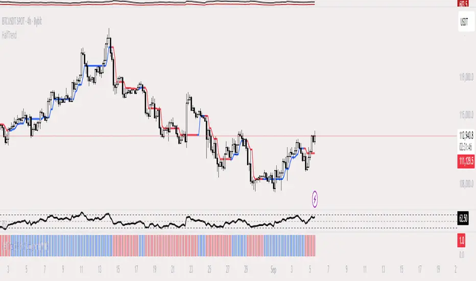
HalfTrend Histogram (MTF)This indicator shows the halftrend on a histogram (rather than a line on the chart) and has an option for Multi timeframe (MTF).
It uses the logic of the original halftrend coded by Everget.
The halftrend is a trend-following indicator that uses volatility to to determine change in bias.
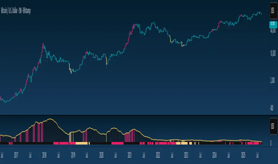
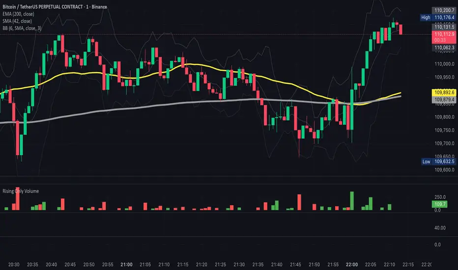
ROV - Rising Only VolumeROV - Rising Only Volume
It will show the volume only if it is above the previous period
Multi-Session High/Low Trackertable that shows rth eth and full weekly range high and low with range difference from high and low

Double Median ATR Bands | MisinkoMasterThe Double Median ATR Bands is a version of the SuperTrend that is designed to be smoother, more accurate while maintaining a good speed by combining the HMA smoothing technique and the median source.
How does it work?
Very simple!
1. Get user defined inputs:
=> Set them up however you want, for the result you want!
2. Calculate the Median of the source and the ATR
=> Very simple
3. Smooth the median with √length (for example if median length = 9, it would be smoothed over the length of 3 since 3x3 = 9)
4. Add ATR bands like so:
Upper = median + (atr*multiplier)
Lower = median - (atr*multiplier)
Trend Logic:
Source crossing over the upper band = uptrend
Source crossing below the lower band = downtrend
Enjoy G´s!

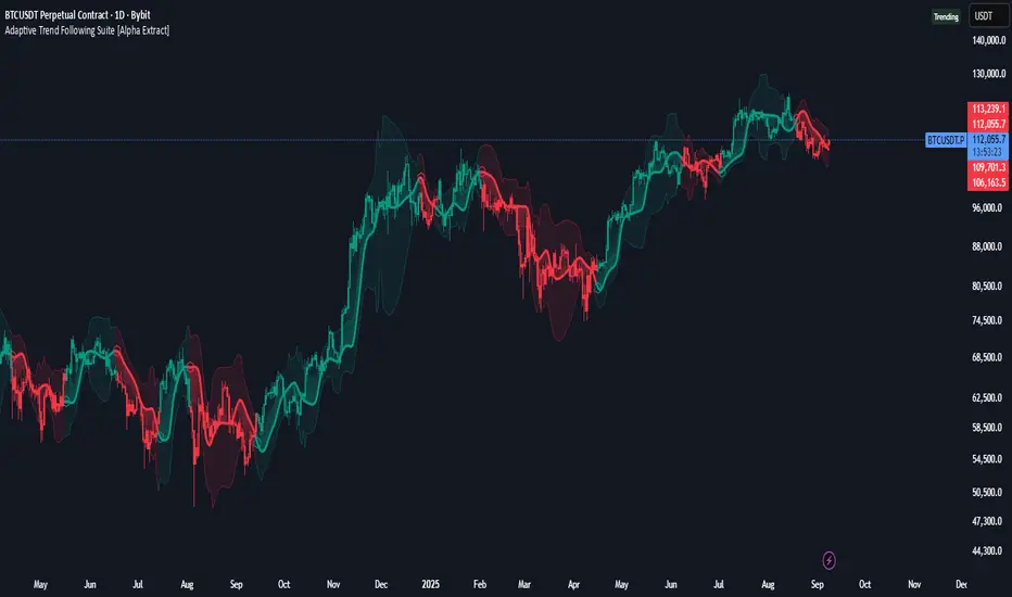
Adaptive Trend Following Suite [Alpha Extract]A sophisticated multi-filter trend analysis system that combines advanced noise reduction, adaptive moving averages, and intelligent market structure detection to deliver institutional-grade trend following signals. Utilizing cutting-edge mathematical algorithms and dynamic channel adaptation, this indicator provides crystal-clear directional guidance with real-time confidence scoring and market mode classification for professional trading execution.
🔶 Advanced Noise Reduction
Filter Eliminates market noise using sophisticated Gaussian filtering with configurable sigma values and period optimization. The system applies mathematical weight distribution across price data to ensure clean signal generation while preserving critical trend information, automatically adjusting filter strength based on volatility conditions.
advancedNoiseFilter(sourceData, filterLength, sigmaParam) =>
weightSum = 0.0
valueSum = 0.0
centerPoint = (filterLength - 1) / 2
for index = 0 to filterLength - 1
gaussianWeight = math.exp(-0.5 * math.pow((index - centerPoint) / sigmaParam, 2))
weightSum += gaussianWeight
valueSum += sourceData * gaussianWeight
valueSum / weightSum
🔶 Adaptive Moving Average Core Engine
Features revolutionary volatility-responsive averaging that automatically adjusts smoothing parameters based on real-time market conditions. The engine calculates adaptive power factors using logarithmic scaling and bandwidth optimization, ensuring optimal responsiveness during trending markets while maintaining stability during consolidation phases.
// Calculate adaptive parameters
adaptiveLength = (periodLength - 1) / 2
logFactor = math.max(math.log(math.sqrt(adaptiveLength)) / math.log(2) + 2, 0)
powerFactor = math.max(logFactor - 2, 0.5)
relativeVol = avgVolatility != 0 ? volatilityMeasure / avgVolatility : 0
adaptivePower = math.pow(relativeVol, powerFactor)
bandwidthFactor = math.sqrt(adaptiveLength) * logFactor
🔶 Intelligent Market Structure Analysis
Employs fractal dimension calculations to classify market conditions as trending or ranging with mathematical precision. The system analyzes price path complexity using normalized data arrays and geometric path length calculations, providing quantitative market mode identification with configurable threshold sensitivity.
🔶 Multi-Component Momentum Analysis
Integrates RSI and CCI oscillators with advanced Z-score normalization for statistical significance testing. Each momentum component receives independent analysis with customizable periods and significance levels, creating a robust consensus system that filters false signals while maintaining sensitivity to genuine momentum shifts.
// Z-score momentum analysis
rsiAverage = ta.sma(rsiComponent, zAnalysisPeriod)
rsiDeviation = ta.stdev(rsiComponent, zAnalysisPeriod)
rsiZScore = (rsiComponent - rsiAverage) / rsiDeviation
if math.abs(rsiZScore) > zSignificanceLevel
rsiMomentumSignal := rsiComponent > 50 ? 1 : rsiComponent < 50 ? -1 : rsiMomentumSignal
❓How It Works
🔶 Dynamic Channel Configuration
Calculates adaptive channel boundaries using three distinct methodologies: ATR-based volatility, Standard Deviation, and advanced Gaussian Deviation analysis. The system automatically adjusts channel multipliers based on market structure classification, applying tighter channels during trending conditions and wider boundaries during ranging markets for optimal signal accuracy.
dynamicChannelEngine(baselineData, channelLength, methodType) =>
switch methodType
"ATR" => ta.atr(channelLength)
"Standard Deviation" => ta.stdev(baselineData, channelLength)
"Gaussian Deviation" =>
weightArray = array.new_float()
totalWeight = 0.0
for i = 0 to channelLength - 1
gaussWeight = math.exp(-math.pow((i / channelLength) / 2, 2))
weightedVariance += math.pow(deviation, 2) * array.get(weightArray, i)
math.sqrt(weightedVariance / totalWeight)
🔶 Signal Processing Pipeline
Executes a sophisticated 10-step signal generation process including noise filtering, trend reference calculation, structure analysis, momentum component processing, channel boundary determination, trend direction assessment, consensus calculation, confidence scoring, and final signal generation with quality control validation.
🔶 Confidence Transformation System
Applies sigmoid transformation functions to raw confidence scores, providing 0-1 normalized confidence ratings with configurable threshold controls. The system uses steepness parameters and center point adjustments to fine-tune signal sensitivity while maintaining statistical robustness across different market conditions.
🔶 Enhanced Visual Presentation
Features dynamic color-coded trend lines with adaptive channel fills, enhanced candlestick visualization, and intelligent price-trend relationship mapping. The system provides real-time visual feedback through gradient fills and transparency adjustments that immediately communicate trend strength and direction changes.
🔶 Real-Time Information Dashboard
Displays critical trading metrics including market mode classification (Trending/Ranging), structure complexity values, confidence scores, and current signal status. The dashboard updates in real-time with color-coded indicators and numerical precision for instant market condition assessment.
🔶 Intelligent Alert System
Generates three distinct alert types: Bullish Signal alerts for uptrend confirmations, Bearish Signal alerts for downtrend confirmations, and Mode Change alerts for market structure transitions. Each alert includes detailed messaging and timestamp information for comprehensive trade management integration.
🔶 Performance Optimization
Utilizes efficient array management and conditional processing to maintain smooth operation across all timeframes. The system employs strategic variable caching, optimized loop structures, and intelligent update mechanisms to ensure consistent performance even during high-volatility market conditions.
This indicator delivers institutional-grade trend analysis through sophisticated mathematical modelling and multi-stage signal processing. By combining advanced noise reduction, adaptive averaging, intelligent structure analysis, and robust momentum confirmation with dynamic channel adaptation, it provides traders with unparalleled trend following precision. The comprehensive confidence scoring system and real-time market mode classification make it an essential tool for professional traders seeking consistent, high-probability trend following opportunities with mathematical certainty and visual clarity.
Deadband Hysteresis Filter [BackQuant]Deadband Hysteresis Filter
What this is
This tool builds a “debounced” price baseline that ignores small fluctuations and only reacts when price meaningfully departs from its recent path. It uses a deadband to define how much deviation matters and a hysteresis scheme to avoid rapid flip-flops around the decision boundary. The baseline’s slope provides a simple trend cue, used to color candles and to trigger up and down alerts.
Why deadband and hysteresis help
They filter micro noise so the baseline does not react to every tiny tick.
They stabilize state changes. Hysteresis means the rule to start moving is stricter than the rule to keep holding, which reduces whipsaw.
They produce a stepped, readable path that advances during sustained moves and stays flat during chop.
How it works (conceptual)
At each bar the script maintains a running baseline dbhf and compares it to the input price p .
Compute a base threshold baseTau using the selected mode (ATR, Percent, Ticks, or Points).
Build an enter band tauEnter = baseTau × Enter Mult and an exit band tauExit = baseTau × Exit Mult where typically Exit Mult < Enter Mult .
Let diff = p − dbhf .
If diff > +tauEnter , raise the baseline by response × (diff − tauEnter) .
If diff < −tauEnter , lower the baseline by response × (diff + tauEnter) .
Otherwise, hold the prior value.
Trend state is derived from slope: dbhf > dbhf → up trend, dbhf < dbhf → down trend.
Inputs and what they control
Threshold mode
ATR — baseTau = ATR(atrLen) × atrMult . Adapts to volatility. Useful when regimes change.
Percent — baseTau = |price| × pctThresh% . Scale-free across symbols of different prices.
Ticks — baseTau = syminfo.mintick × tickThresh . Good for futures where tick size matters.
Points — baseTau = ptsThresh . Fixed distance in price units.
Band multipliers and response
Enter Mult — outer band. Price must travel at least this far from the baseline before an update occurs. Larger values reject more noise but increase lag.
Exit Mult — inner band for hysteresis. Keep this smaller than Enter Mult to create a hold zone that resists small re-entries.
Response — step size when outside the enter band. Higher response tracks faster; lower response is smoother.
UI settings
Show Filtered Price — plots the baseline on price.
Paint candles — colors bars by the filtered slope using your long/short colors.
How it can be used
Trend qualifier — take entries only in the direction of the baseline slope and skip trades against it.
Debounced crossovers — use the baseline as a stabilized surrogate for price in moving-average or channel crossover rules.
Trailing logic — trail stops a small distance beyond the baseline so small pullbacks do not eject the trade.
Session aware filtering — widen Enter Mult or switch to ATR mode for volatile sessions; tighten in quiet sessions.
Parameter interactions and tuning
Enter Mult vs Response — both govern sensitivity. If you see too many flips, increase Enter Mult or reduce Response. If turns feel late, do the opposite.
Exit Mult — widening the gap between Enter and Exit expands the hold zone and reduces oscillation around the threshold.
Mode choice — ATR adapts automatically; Percent keeps behavior consistent across instruments; Ticks or Points are useful when you think in fixed increments.
Timeframe coupling — on higher timeframes you can often lower Enter Mult or raise Response because raw noise is already reduced.
Concrete starter recipes
General purpose — ATR mode, atrLen=14 , atrMult=1.0–1.5 , Enter=1.0 , Exit=0.5 , Response=0.20 . Balanced noise rejection and lag.
Choppy range filter — ATR mode, increase atrMult to 2.0, keep Response≈0.15 . Stronger suppression of micro-moves.
Fast intraday — Percent mode, pctThresh=0.1–0.3 , Enter=1.0 , Exit=0.4–0.6 , Response=0.30–0.40 . Quicker turns for scalping.
Futures ticks — Ticks mode, set tickThresh to a few spreads beyond typical noise; start with Enter=1.0 , Exit=0.5 , Response=0.25 .
Strengths
Clear, explainable logic with an explicit noise budget.
Multiple threshold modes so the same tool fits equities, futures, and crypto.
Built-in hysteresis that reduces flip-flop near the boundary.
Slope-based coloring and alerts that make state changes obvious in real time.
Limitations and notes
All filters add lag. Larger thresholds and smaller response trade faster reaction for fewer false turns.
Fixed Points or Ticks can under- or over-filter when volatility regime shifts. ATR adapts, but will also expand bands during spikes.
On extremely choppy symbols, even a well tuned band will step frequently. Widen Enter Mult or reduce Response if needed.
This is a chart study. It does not include commissions, slippage, funding, or gap risks.
Alerts
DBHF Up Slope — baseline turns from down to up on the latest bar.
DBHF Down Slope — baseline turns from up to down on the latest bar.
Implementation details worth knowing
Initialization sets the baseline to the first observed price to avoid a cold-start jump.
Slope is evaluated bar-to-bar. The up and down alerts check for a change of slope rather than raw price crossings.
Candle colors and the baseline plot share the same long/short palette with transparency applied to the line.
Practical workflow
Pick a mode that matches how you think about distance. ATR for volatility aware, Percent for scale-free, Ticks or Points for fixed increments.
Tune Enter Mult until the number of flips feels appropriate for your timeframe.
Set Exit Mult clearly below Enter Mult to create a real hold zone.
Adjust Response last to control “how fast” the baseline chases price once it decides to move.
Final thoughts
Deadband plus hysteresis gives you a principled way to “only care when it matters.” With a sensible threshold and response, the filter yields a stable, low-chop trend cue you can use directly for bias or plug into your own entries, exits, and risk rules.

2ATR / Close %Certainly. Here is the English version of the indicator description you requested.
---
### **2ATR Stop-Loss Ratio**
This indicator provides a straightforward calculation of **what percentage a 2ATR (Average True Range) move represents relative to the current price**. It's a specialized tool designed to help traders set dynamic, volatility-based stop-loss levels.
---
### **Purpose of the Indicator**
Many traders use a **2ATR** as their standard for setting a stop-loss, believing it's a good measure of a stock's typical movement. However, it can be difficult to quickly determine the exact percentage a 2ATR drop represents from the current price. This indicator solves that problem by giving you a clear, single number that shows the **anticipated percentage loss before you even enter a position**.
---
### **How It Works**
The indicator is calculated using a simple formula:
**(2 * ATR(20) / Current Price) * 100**
* `ATR(20)`: The Average True Range over the last 20 periods. This period can be customized in the indicator's settings.
* `Current Price`: The closing price at the time of calculation.
---
### **How to Use It**
* **Assess Risk**: A higher number on the indicator means greater volatility, indicating a wider stop-loss range.
* **Set a Stop-Loss**: If the indicator shows **3%**, it means a 2ATR move is roughly a 3% change from the current price. This gives you a clear understanding of the potential loss.
* **Adjust Position Size**: If the potential percentage loss is larger than you're comfortable with, you can use this information to reduce your position size, effectively managing your risk.
This tool is especially useful for trading highly volatile stocks, as it helps you establish a clear and effective risk management strategy.

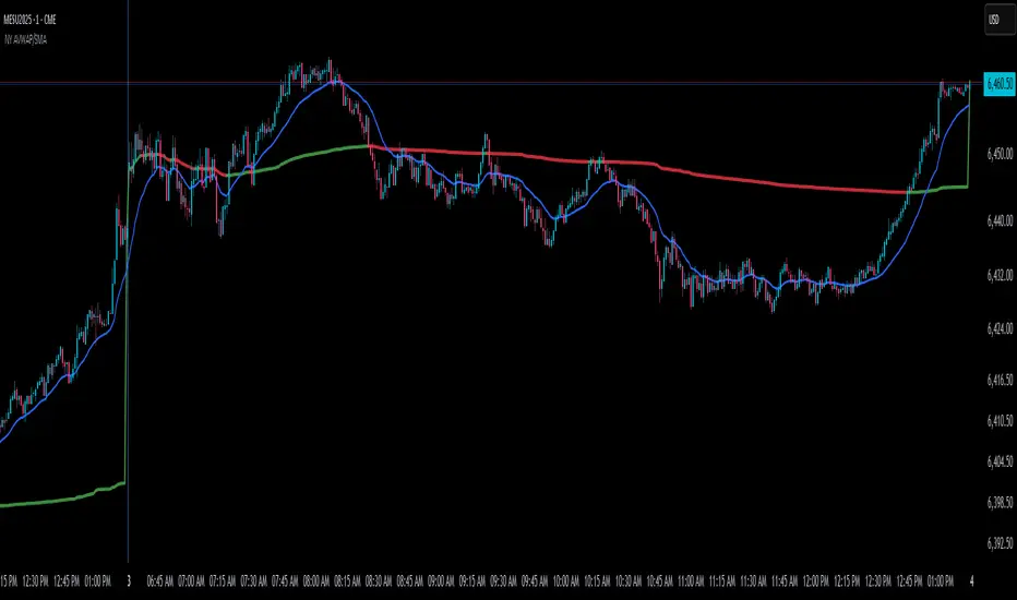
NY Anchored VWAP and Auto SMANY Anchored VWAP and Auto SMA
This script is a versatile trading indicator for the TradingView platform that combines two powerful components: a New York-anchored Volume-Weighted Average Price (VWAP) and a dynamic Simple Moving Average (SMA). Designed for traders who utilize VWAP for intraday trend analysis, this tool provides a clear visual representation of average price and volatility-adjusted moving averages, generating automated alerts for key crossover signals.
Indicator Components
1. NY Anchored VWAP
The VWAP is a crucial tool that represents the average price of a security adjusted for volume. This version is "anchored" to the start of the New York trading session, resetting at the beginning of each new session. This provides a clean, session-specific anchor point to gauge market sentiment and trend. The VWAP line changes color to reflect its slope:
Green: When the VWAP is trending upwards, indicating a bullish bias.
Red: When the VWAP is trending downwards, indicating a bearish bias.
2. Auto SMA
The Auto SMA is a moving average with a unique twist: its lookback period is not fixed. Instead, it dynamically adjusts based on market volatility. The script measures volatility using the Average True Range (ATR) and a Z-Score calculation.
When volatility is expanding, the SMA's length shortens, making it more sensitive to recent price changes.
When volatility is contracting, the SMA's length lengthens, smoothing out the price action to filter out noise.
This adaptive approach allows the SMA to react appropriately to different market conditions.
Suggested Trading Strategy
This indicator is particularly effective when used on a one-minute chart for identifying high-probability trade entries. The core of the strategy is to trade the crossover between the VWAP and the Auto SMA, with confirmation from a candle close.
The strategy works best when the entry signal aligns with the overall bias of the higher timeframe market structure. For example, if the daily or 4-hour chart is in an uptrend, you would look for bullish signals on the one-minute chart.
Bullish Entry Signal: A potential entry is signaled when the VWAP crosses above the Auto SMA, and is confirmed when the one-minute candle closes above both the VWAP and the SMA. This indicates a potential continuation of the bullish momentum.
Bearish Entry Signal: A potential entry is signaled when the VWAP crosses below the Auto SMA, and is confirmed when the one-minute candle closes below both the VWAP and the SMA. This indicates a potential continuation of the bearish momentum.
The built-in alerts for these crossovers allow you to receive notifications without having to constantly monitor the charts, ensuring you don't miss a potential setup.
Triple Tap Sniper Triple Tap Sniper v3 – EMA Retest Precision System
Triple Tap Sniper is a precision trading tool built around the 21, 34, and 55 EMAs, designed to capture high-probability retests after EMA crosses. Instead of chasing the first breakout candle, the system waits for the first pullback into the EMA21 after a trend-confirming cross — the spot where professional traders often enter.
🔑 Core Logic
EMA Alignment → Trend defined by EMA21 > EMA34 > EMA55 (bullish) or EMA21 < EMA34 < EMA55 (bearish).
Cross Detection → Signals are only armed after a fresh EMA cross.
Retest Entry → Buy/Sell signals fire only on the first retest of EMA21, with trend still intact.
Pro Filters →
📊 Higher Timeframe Confirmation: Aligns signals with larger trend.
📈 ATR Volatility Filter: Blocks weak signals in low-vol chop.
📏 EMA Spread Filter: Ignores tiny “fake crosses.”
🕯️ Price Action Filter: Requires a proper wick rejection for valid entries.
🚀 Why Use Triple Tap Sniper?
✅ Filters out most false signals from sideways markets.
✅ Focuses only on clean trend continuations after pullbacks.
✅ Beginner-friendly visuals (Buy/Sell labels) + alert-ready for automation.
✅ Flexible: works across multiple timeframes & asset classes (stocks, crypto, forex).
⚠️ Notes
This is a signal indicator, not a full strategy. For backtesting and optimization, convert to a strategy and adjust filters per market/timeframe.
No indicator guarantees profits — use with sound risk management.

Perfect Price-Anchored % Fib Grid This indicator generates support and resistance levels anchored to a fixed price of your choice.
You can also specify a percentage for the indicator to calculate potential highs and lows.
Commonly used values are 3.5% or 7%, as well as smaller decimal versions like 0.35% or 0.7%, depending on the volatility you expect.
In addition, the indicator can highlight potential stop-run levels in multiples of 27 — ranging from 0 up to 243. This automatically places the 243 GB range directly onto your chart.
The tool is versatile and can be applied not only to equities, but also to ES futures and Forex markets.
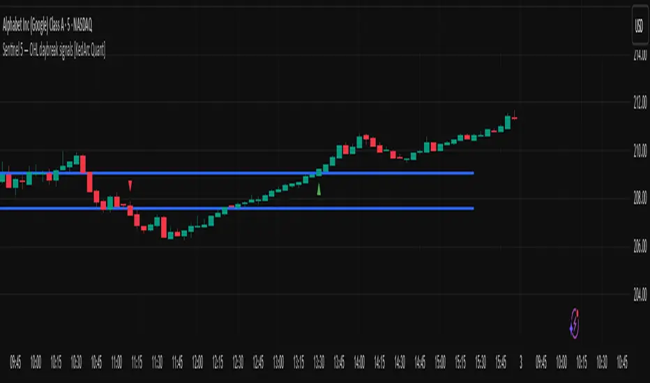
Sentinel 5 — OHL daybreak signals [KedArc Quant]Overview
Sentinel 5 plots the first-bar high/low of each trading session and gives clean, rules-based signals in two ways:
1) OHL Setups at the close of the first bar (Open equals/near High for potential short; Open equals/near Low for potential long).
2) Breakout Signals later in the session when price breaks the first-bar High/Low, with optional body/penetration filters.
Basic workflow
1. Wait for the first session bar to finish.
*If O≈H (optionally by proximity) → short setup. •
*If O≈L → long setup. • If neither happens, optionally allow later breakouts.
2. Optional: Act only on breakouts that penetrate a minimum % of that bar’s range/body.
3. Skip the day automatically if the first bar is abnormally large (marubozu-like / extreme ATR / outsized vs yesterday).
Signals & Markers
Markers on the chart:
▲ O=L (exact) / O near L (proximity) – long setup at first-bar close.
▼ O=H (exact) / O near H (proximity) – short setup at first-bar close.
▲ Breakout Long – later bar breaks above first-bar High meeting your penetration rule.
▼ Breakout Short – later bar breaks below first-bar Low meeting your penetration rule.
ATR% | Volatility NormalizerThis indicator measures true volatility by expressing the Average True Range (ATR) as a percentage of price. Unlike basic ATR plots, which show raw values, this version normalizes volatility to make it directly comparable across instruments and timeframes.
How it works:
Uses True Range (High–Low plus gaps) to capture actual market movement.
Normalizes by dividing ATR by the chosen price base (default: Close).
Multiplies by 100 to output a clean ATR% line.
Smoothing is flexible: choose from RMA, SMA, EMA, or WMA.
Optional Feature:
For comparison, you can toggle an auxiliary line showing the average absolute close-to-close % move, highlighting the difference between simplified and true volatility.
Why use it:
Track regime shifts: identify when volatility expands or contracts in % terms.
Compare volatility across different markets (equities, crypto, forex, commodities).
Integrate into risk management: position sizing, stop placement, or volatility filters for entries.
Interpretation:
Rising ATR% → expanding volatility, potential breakouts or unstable ranges.
Falling ATR% → contracting volatility, possible consolidation or range-bound conditions.
Sudden spikes → market “shocks” worth paying attention to.

Volatility % Bands (O→C)Volatility % Bands (O→C) is an indicator designed to visualize the percentage change from Open to Close of each candle, providing a clear view of short-term momentum and volatility.
**Histogram**: Displays bar-by-bar % change (Close vs Open). Green bars indicate positive changes, while red bars indicate negative ones, making momentum shifts easy to identify.
**Moving Average Line**: Plots the Simple Moving Average (SMA) of the absolute % change, helping traders track the average volatility over a chosen period.
**Background Bands**: Based on the user-defined Level Step, ±1 to ±5 zones are highlighted as shaded bands, allowing quick recognition of whether volatility is low, moderate, or extreme.
**Label**: Shows the latest candle’s % change and the current SMA value as a floating label on the right, making it convenient for real-time monitoring.
This tool can be useful for volatility breakout strategies, day trading, and short-term momentum analysis.