Prophet Model [TakingProphets]The Prophet Model — context pipeline (HTF PDA → Sweep → CISD → EPE) with dynamic risk
Purpose
Informational overlay for organizing institutional context in real time. It does not issue buy/sell signals and is not financial advice. Use it to structure analysis and checklist-driven execution—not to automate decisions.
What it does (modules at a glance)
Projects HTF PD Arrays (FVGs) onto your current chart and maintains only the nearest active array.
Validates directional bias using Candle Range Theory (CRT) on the same HTF.
Tracks Liquidity Sweeps (BSL/SSL) on HTF-aware pivots.
Confirms Change in State of Delivery (CISD) via displacement after a sweep.
Optionally refines entries with EPE when a local (internal) imbalance forms right after CISD.
Derives dynamic TP/BE/SL from measured displacement and recent extremes (not fixed distances).
Keeps a rules checklist (PDA tap → CRT → Sweep → CISD) and a relationships table (common HTF↔LTF pairings) to enforce process.
How it works (integration, not a mashup)
The modules are sequenced on one HTF time base so each step gates the next:
HTF PD Arrays (context zone). The model identifies valid HTF FVGs, filters tiny/weekend gaps, removes arrays that are invalidated by clean trades-through, and persists only the nearest PDA. This focuses attention on the institutional zone most likely to matter now.
CRT (directional gating). CRT on the same HTF establishes a provisional bias. No entries are implied; CRT simply permits or forbids the following steps. If CRT disagrees with the PDA context, the checklist remains incomplete.
Liquidity Sweep (event). The model tracks HTF-aware BSL/SSL pivots. A sweep only “counts” if it occurs in relation to the active PDA (tap/engagement). This prevents generic swing-high/low tags from triggering downstream logic.
CISD (confirmation). After a qualified sweep, the tool looks for displacement through the sequence open (the open of the impulsive leg beginning at or immediately after the sweep). Crossing that threshold confirms CISD, which marks a structural delivery shift consistent with the CRT bias.
EPE (refinement, optional). Immediately following CISD, the model scans for a fresh internal imbalance. If found quickly, it promotes that price area as the Easiest Point of Entry (EPE) and relabels the reference. If not, the CISD level remains primary.
Dynamic risk levels. TP/BE/SL are derived from the measured displacement around the CISD leg (e.g., BE ≈ 1× leg, TP ≈ 2.25× stretch; SL aligned to nearby structural extremes rather than a fixed pip offset). Levels update with structure and can display prices.
By chaining PDA → CRT → Sweep → CISD → (EPE) → Risk on a single HTF backbone, the tool creates a coherent workflow where later signals simply do not appear without earlier context. That’s why this is not a bundle of independent features: each module’s output is another module’s input.
Concepts & operational rules (high level)
HTF PD Arrays (FVGs)
Uses a standard three-candle gap definition on the chosen HTF, with filters for weekend/tiny gaps.
Inverse mitigation: if price trades cleanly through an array, the box is removed and internal state resets.
Nearest-PDA persistence: when multiple arrays exist, only the closest remains visible to reduce clutter.
Optional right-extension draws lingering influence X bars forward.
Candle Range Theory (CRT)
Bullish CRT: candle 2 wicks below candle 1’s low but closes back inside candle 1’s range, without taking its high.
Bearish CRT: candle 2 wicks above candle 1’s high but closes back inside candle 1’s range, without taking its low.
Role: bias validation paired to CISD when alignments match the active PDA.
Liquidity Sweeps (BSL/SSL)
Tracks candidate HTF pivots as buy-/sell-side liquidity.
A sweep registers when price takes a tracked pivot in the vicinity of the active PDA.
CISD (Change in State of Delivery)
Finds the sequence open for the impulsive leg that begins at/after the sweep.
Bearish path (after BSL sweep): CISD when close < sequence-open.
Bullish path (after SSL sweep): CISD when close > sequence-open.
On confirmation, the model plots a CISD line, checks the box in the Strategy Checklist, and triggers risk calc.
EPE (Easiest Point of Entry)
Within a short window after CISD, scans for a local imbalance; if present, promotes that level as EPE.
If no imbalance forms, CISD remains the operative reference.
Dynamic TP / BE / SL
Built from the measured leg around CISD (not fixed pip steps).
Approximate geometry: BE ≈ 1× leg, TP ≈ 2.25× leg; SL respects nearby structural extremes.
Labels and price markers are optional.
Architecture notes
Maps the current chart to a higher timeframe (e.g., 15s→M5, M1→M15, M5→H1, M15→H4, H1→D, H4→W, D→M).
Retrieves HTF OHLC/time with no lookahead so structures update intrabar until the HTF bar closes.
Periodic cleanup clears obsolete lines/labels/boxes to keep charts responsive.
Inputs (summary)
FVGs/PD Arrays: show/hide, colors, borders, label size, right-extension, nearest-only toggle.
CRT: enable/disable, label style.
Sweeps/CISD/EPE: enable/disable, line/label styles, EPE window.
Risk Levels (TP/BE/SL): enable each, price labels on/off, colors.
Tables/Checklist: strategy checklist on/off; relationships table (common HTF↔LTF pairings); text sizes and header colors.
Alerts (optional)
You may add alertconditions aligned with these events in your own workspace:
HTF PDA tap (bullish/bearish box)
CRT detected (bullish/bearish)
CISD confirmed (bullish/bearish)
EPE set/updated
Example messages:
“Prophet: CISD confirmed on {{ticker}} / {{interval}}”
“Prophet: EPE refined at {{close}} ({{time}})”
Notes & limitations
HTF values are provisional until the HTF bar closes; labels/levels can update while forming.
CISD/EPE are live conditions; they can form and later invalidate within the same HTF bar.
Liquidity relationships vary by market/regime; thin sessions and large gaps can affect clarity.
Educational tool only. No performance claims; no trade signals.
Originality & scope (for protected/invite-only publications)
A single HTF-synchronized engine sequences PDA → CRT → Sweep → CISD → (EPE) and withholds later steps unless prerequisites are met.
Nearest-PDA persistence and inverse-mitigation enforce focus on the most relevant institutional zone.
Displacement-based risk math ties TP/BE/SL to structure instead of static offsets.
Checklist + relationships table promote consistent, rules-first behavior and reduce discretionary drift.
Attribution: Concepts inspired by ICT (PD arrays/FVGs, CRT, sweeps, displacement, refined entries). Design, integration logic, and risk framework by TakingProphets.
Pesquisar nos scripts por "track"

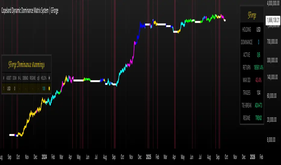
Copeland Dynamic Dominance Matrix System | GForgeCopeland Dynamic Dominance Matrix System | GForge - v1
---
📊 COMPREHENSIVE SYSTEM OVERVIEW
The GForge Dynamic BB% TrendSync System represents a revolutionary approach to algorithmic portfolio management, combining cutting-edge statistical analysis, momentum detection, and regime identification into a unified framework. This system processes up to 39 different cryptocurrency assets simultaneously, using advanced mathematical models to determine optimal capital allocation across dynamic market conditions.
Core Innovation: Multi-Dimensional Analysis
Unlike traditional single-asset indicators, this system operates on multiple analytical dimensions:
Momentum Analysis: Dual Bollinger Band Modified Deviation (DBBMD) calculations
Relative Strength: Comprehensive dominance matrix with head-to-head comparisons
Fundamental Screening: Alpha and Beta statistical filtering
Market Regime Detection: Five-component statistical testing framework
Portfolio Optimization: Dynamic weighting and allocation algorithms
Risk Management: Multi-layered protection and regime-based positioning
---
🔧 DETAILED COMPONENT BREAKDOWN
1. Dynamic Bollinger Band % Modified Deviation Engine (DBBMD)
The foundation of this system is an advanced oscillator that combines two independent Bollinger Band systems with asymmetric parameters to create unique momentum readings.
Technical Implementation:
[
// BB System 1: Fast-reacting with extended standard deviation
primary_bb1_ma_len = 40 // Shorter MA for responsiveness
primary_bb1_sd_len = 65 // Longer SD for stability
primary_bb1_mult = 1.0 // Standard deviation multiplier
// BB System 2: Complementary asymmetric design
primary_bb2_ma_len = 8 // Longer MA for trend following
primary_bb2_sd_len = 66 // Shorter SD for volatility sensitivity
primary_bb2_mult = 1.7 // Wider bands for reduced noise
Key Features:
Asymmetric Design: The intentional mismatch between MA and Standard Deviation periods creates unique oscillation characteristics that traditional Bollinger Bands cannot achieve
Percentage Scale: All readings are normalized to 0-100% scale for consistent interpretation across assets
Multiple Combination Modes:
BB1 Only: Fast/reactive system
BB2 Only: Smooth/stable system
Average: Balanced blend (recommended)
Both Required: Conservative (both must agree)
Either One: Aggressive (either can trigger)
Mean Deviation Filter: Additional volatility-based layer that measures the standard deviation of the DBBMD% itself, creating dynamic trigger bands
Signal Generation Logic:
// Primary thresholds
primary_long_threshold = 71 // DBBMD% level for bullish signals
primary_short_threshold = 33 // DBBMD% level for bearish signals
// Mean Deviation creates dynamic bands around these thresholds
upper_md_band = combined_bb + (md_mult * bb_std)
lower_md_band = combined_bb - (md_mult * bb_std)
// Signal triggers when DBBMD crosses these dynamic bands
long_signal = lower_md_band > long_threshold
short_signal = upper_md_band < short_threshold
For more information on this BB% indicator, find it here:
2. Revolutionary Dominance Matrix System
This is the system's most sophisticated innovation - a comprehensive framework that compares every asset against every other asset to determine relative strength hierarchies.
Mathematical Foundation:
The system constructs a mathematical matrix where each cell represents whether asset i dominates asset j:
// Core dominance matrix (39x39 for maximum assets)
var matrix dominance_matrix = matrix.new(39, 39, 0)
// For each qualifying asset pair (i,j):
for i = 0 to active_count - 1
for j = 0 to active_count - 1
if i != j
// Calculate price ratio BB% TrendSync for asset_i/asset_j
ratio_array = calculate_price_ratios(asset_i, asset_j)
ratio_dbbmd = calculate_dbbmd(ratio_array)
// Asset i dominates j if ratio is in uptrend
if ratio_dbbmd_state == 1
matrix.set(dominance_matrix, i, j, 1)
Copeland Scoring Algorithm:
Each asset receives a dominance score calculated as:
Dominance Score = Total Wins - Total Losses
// Calculate net dominance for each asset
for i = 0 to active_count - 1
wins = 0
losses = 0
for j = 0 to active_count - 1
if i != j
if matrix.get(dominance_matrix, i, j) == 1
wins += 1
else
losses += 1
copeland_score = wins - losses
array.set(dominance_scores, i, copeland_score)
Head-to-Head Analysis Process:
Ratio Construction: For each asset pair, calculate price_asset_A / price_asset_B
DBBMD Application: Apply the same DBBMD analysis to these ratios
Trend Determination: If ratio DBBMD shows uptrend, Asset A dominates Asset B
Matrix Population: Store dominance relationships in mathematical matrix
Score Calculation: Sum wins minus losses for final ranking
This creates a tournament-style ranking where each asset's strength is measured against all others, not just against a benchmark.
3. Advanced Alpha & Beta Filtering System
The system incorporates fundamental analysis through Capital Asset Pricing Model (CAPM) calculations to filter assets based on risk-adjusted performance.
Alpha Calculation (Excess Return Analysis):
// CAPM Alpha calculation
f_calc_alpha(asset_prices, benchmark_prices, alpha_length, beta_length, risk_free_rate) =>
// Calculate asset and benchmark returns
asset_returns = calculate_returns(asset_prices, alpha_length)
benchmark_returns = calculate_returns(benchmark_prices, alpha_length)
// Get beta for expected return calculation
beta = f_calc_beta(asset_prices, benchmark_prices, beta_length)
// Average returns over period
avg_asset_return = array_average(asset_returns) * 100
avg_benchmark_return = array_average(benchmark_returns) * 100
// Expected return using CAPM: E(R) = Beta * Market_Return + Risk_Free_Rate
expected_return = beta * avg_benchmark_return + risk_free_rate
// Alpha = Actual Return - Expected Return
alpha = avg_asset_return - expected_return
Beta Calculation (Volatility Relationship):
// Beta measures how much an asset moves relative to benchmark
f_calc_beta(asset_prices, benchmark_prices, length) =>
// Calculate return series for both assets
asset_returns =
benchmark_returns =
// Populate return arrays
for i = 0 to length - 1
asset_return = (current_price - previous_price) / previous_price
benchmark_return = (current_bench - previous_bench) / previous_bench
// Calculate covariance and variance
covariance = calculate_covariance(asset_returns, benchmark_returns)
benchmark_variance = calculate_variance(benchmark_returns)
// Beta = Covariance(Asset, Market) / Variance(Market)
beta = covariance / benchmark_variance
Filtering Applications:
Alpha Filter: Only includes assets with alpha above specified threshold (e.g., >0.5% monthly excess return)
Beta Filter: Screens for desired volatility characteristics (e.g., beta >1.0 for aggressive assets)
Combined Screening: Both filters must pass for asset qualification
Dynamic Thresholds: User-configurable parameters for different market conditions
4. Intelligent Tie-Breaking Resolution System
When multiple assets have identical dominance scores, the system employs sophisticated methods to determine final rankings.
Standard Tie-Breaking Hierarchy:
// Primary tie-breaking logic
if score_i == score_j // Tied dominance scores
// Level 1: Compare Beta values (higher beta wins)
beta_i = array.get(beta_values, i)
beta_j = array.get(beta_values, j)
if beta_j > beta_i
swap_positions(i, j)
else if beta_j == beta_i
// Level 2: Compare Alpha values (higher alpha wins)
alpha_i = array.get(alpha_values, i)
alpha_j = array.get(alpha_values, j)
if alpha_j > alpha_i
swap_positions(i, j)
Advanced Tie-Breaking (Head-to-Head Analysis):
For the top 3 performers, an enhanced tie-breaking mechanism analyzes direct head-to-head price ratio performance:
// Advanced tie-breaker for top performers
f_advanced_tiebreaker(asset1_idx, asset2_idx, lookback_period) =>
// Calculate price ratio over lookback period
ratio_history =
for k = 0 to lookback_period - 1
price_ratio = price_asset1 / price_asset2
array.push(ratio_history, price_ratio)
// Apply simplified trend analysis to ratio
current_ratio = array.get(ratio_history, 0)
average_ratio = calculate_average(ratio_history)
// Asset 1 wins if current ratio > average (trending up)
if current_ratio > average_ratio
return 1 // Asset 1 dominates
else
return -1 // Asset 2 dominates
5. Five-Component Aggregate Market Regime Filter
This sophisticated framework combines multiple statistical tests to determine whether market conditions favor trending strategies or require defensive positioning.
Component 1: Augmented Dickey-Fuller (ADF) Test
Tests for unit root presence to distinguish between trending and mean-reverting price series.
// Simplified ADF implementation
calculate_adf_statistic(price_series, lookback) =>
// Calculate first differences
differences =
for i = 0 to lookback - 2
diff = price_series - price_series
array.push(differences, diff)
// Statistical analysis of differences
mean_diff = calculate_mean(differences)
std_diff = calculate_standard_deviation(differences)
// ADF statistic approximation
adf_stat = mean_diff / std_diff
// Compare against threshold for trend determination
is_trending = adf_stat <= adf_threshold
Component 2: Directional Movement Index (DMI)
Classic Wilder indicator measuring trend strength through directional movement analysis.
// DMI calculation for trend strength
calculate_dmi_signal(high_data, low_data, close_data, period) =>
// Calculate directional movements
plus_dm_sum = 0.0
minus_dm_sum = 0.0
true_range_sum = 0.0
for i = 1 to period
// Directional movements
up_move = high_data - high_data
down_move = low_data - low_data
// Accumulate positive/negative movements
if up_move > down_move and up_move > 0
plus_dm_sum += up_move
if down_move > up_move and down_move > 0
minus_dm_sum += down_move
// True range calculation
true_range_sum += calculate_true_range(i)
// Calculate directional indicators
di_plus = 100 * plus_dm_sum / true_range_sum
di_minus = 100 * minus_dm_sum / true_range_sum
// ADX calculation
dx = 100 * math.abs(di_plus - di_minus) / (di_plus + di_minus)
adx = dx // Simplified for demonstration
// Trending if ADX above threshold
is_trending = adx > dmi_threshold
Component 3: KPSS Stationarity Test
Complementary test to ADF that examines stationarity around trend components.
// KPSS test implementation
calculate_kpss_statistic(price_series, lookback, significance_level) =>
// Calculate mean and variance
series_mean = calculate_mean(price_series, lookback)
series_variance = calculate_variance(price_series, lookback)
// Cumulative sum of deviations
cumulative_sum = 0.0
cumsum_squared_sum = 0.0
for i = 0 to lookback - 1
deviation = price_series - series_mean
cumulative_sum += deviation
cumsum_squared_sum += math.pow(cumulative_sum, 2)
// KPSS statistic
kpss_stat = cumsum_squared_sum / (lookback * lookback * series_variance)
// Compare against critical values
critical_value = significance_level == 0.01 ? 0.739 :
significance_level == 0.05 ? 0.463 : 0.347
is_trending = kpss_stat >= critical_value
Component 4: Choppiness Index
Measures market directionality using fractal dimension analysis of price movement.
// Choppiness Index calculation
calculate_choppiness(price_data, period) =>
// Find highest and lowest over period
highest = price_data
lowest = price_data
true_range_sum = 0.0
for i = 0 to period - 1
if price_data > highest
highest := price_data
if price_data < lowest
lowest := price_data
// Accumulate true range
if i > 0
true_range = calculate_true_range(price_data, i)
true_range_sum += true_range
// Choppiness calculation
range_high_low = highest - lowest
choppiness = 100 * math.log10(true_range_sum / range_high_low) / math.log10(period)
// Trending if choppiness below threshold (typically 61.8)
is_trending = choppiness < 61.8
Component 5: Hilbert Transform Analysis
Phase-based cycle detection and trend identification using mathematical signal processing.
// Hilbert Transform trend detection
calculate_hilbert_signal(price_data, smoothing_period, filter_period) =>
// Smooth the price data
smoothed_price = calculate_moving_average(price_data, smoothing_period)
// Calculate instantaneous phase components
// Simplified implementation for demonstration
instant_phase = smoothed_price
delayed_phase = calculate_moving_average(price_data, filter_period)
// Compare instantaneous vs delayed signals
phase_difference = instant_phase - delayed_phase
// Trending if instantaneous leads delayed
is_trending = phase_difference > 0
Aggregate Regime Determination:
// Combine all five components
regime_calculation() =>
trending_count = 0
total_components = 0
// Test each enabled component
if enable_adf and adf_signal == 1
trending_count += 1
if enable_adf
total_components += 1
// Repeat for all five components...
// Calculate trending proportion
trending_proportion = trending_count / total_components
// Market is trending if proportion above threshold
regime_allows_trading = trending_proportion >= regime_threshold
The system only allows asset positions when the specified percentage of components indicate trending conditions. During choppy or mean-reverting periods, the system automatically positions in USD to preserve capital.
6. Dynamic Portfolio Weighting Framework
Six sophisticated allocation methodologies provide flexibility for different market conditions and risk preferences.
Weighting Method Implementations:
1. Equal Weight Distribution:
// Simple equal allocation
if weighting_mode == "Equal Weight"
weight_per_asset = 1.0 / selection_count
for i = 0 to selection_count - 1
array.push(weights, weight_per_asset)
2. Linear Dominance Scaling:
// Linear scaling based on dominance scores
if weighting_mode == "Linear Dominance"
// Normalize scores to 0-1 range
min_score = array.min(dominance_scores)
max_score = array.max(dominance_scores)
score_range = max_score - min_score
total_weight = 0.0
for i = 0 to selection_count - 1
score = array.get(dominance_scores, i)
normalized = (score - min_score) / score_range
weight = 1.0 + normalized * concentration_factor
array.push(weights, weight)
total_weight += weight
// Normalize to sum to 1.0
for i = 0 to selection_count - 1
current_weight = array.get(weights, i)
array.set(weights, i, current_weight / total_weight)
3. Conviction Score (Exponential):
// Exponential scaling for high conviction
if weighting_mode == "Conviction Score"
// Combine dominance score with DBBMD strength
conviction_scores =
for i = 0 to selection_count - 1
dominance = array.get(dominance_scores, i)
dbbmd_strength = array.get(dbbmd_values, i)
conviction = dominance + (dbbmd_strength - 50) / 25
array.push(conviction_scores, conviction)
// Exponential weighting
total_weight = 0.0
for i = 0 to selection_count - 1
conviction = array.get(conviction_scores, i)
normalized = normalize_score(conviction)
weight = math.pow(1 + normalized, concentration_factor)
array.push(weights, weight)
total_weight += weight
// Final normalization
normalize_weights(weights, total_weight)
Advanced Features:
Minimum Position Constraint: Prevents dust allocations below specified threshold
Concentration Factor: Adjustable parameter controlling weight distribution aggressiveness
Dominance Boost: Extra weight for assets exceeding specified dominance thresholds
Dynamic Rebalancing: Automatic weight recalculation on portfolio changes
7. Intelligent USD Management System
The system treats USD as a competing asset with its own dominance score, enabling sophisticated cash management.
USD Scoring Methodologies:
Smart Competition Mode (Recommended):
f_calculate_smart_usd_dominance() =>
usd_wins = 0
// USD beats assets in downtrends or weak uptrends
for i = 0 to active_count - 1
asset_state = get_asset_state(i)
asset_dbbmd = get_asset_dbbmd(i)
// USD dominates shorts and weak longs
if asset_state == -1 or (asset_state == 1 and asset_dbbmd < long_threshold)
usd_wins += 1
// Calculate Copeland-style score
base_score = usd_wins - (active_count - usd_wins)
// Boost during weak market conditions
qualified_assets = count_qualified_long_assets()
if qualified_assets <= active_count * 0.2
base_score := math.round(base_score * usd_boost_factor)
base_score
Auto Short Count Mode:
// USD dominance based on number of bearish assets
usd_dominance = count_assets_in_short_state()
// Apply boost during low activity
if qualified_long_count <= active_count * 0.2
usd_dominance := usd_dominance * usd_boost_factor
Regime-Based USD Positioning:
When the five-component regime filter indicates unfavorable conditions, the system automatically overrides all asset signals and positions 100% in USD, protecting capital during choppy markets.
8. Multi-Asset Infrastructure & Data Management
The system maintains comprehensive data structures for up to 39 assets simultaneously.
Data Collection Framework:
// Full OHLC data matrices (200 bars depth for performance)
var matrix open_data = matrix.new(39, 200, na)
var matrix high_data = matrix.new(39, 200, na)
var matrix low_data = matrix.new(39, 200, na)
var matrix close_data = matrix.new(39, 200, na)
// Real-time data collection
if barstate.isconfirmed
for i = 0 to active_count - 1
ticker = array.get(assets, i)
= request.security(ticker, timeframe.period,
[open , high , low , close ],
lookahead=barmerge.lookahead_off)
// Store in matrices with proper shifting
matrix.set(open_data, i, 0, nz(o, 0))
matrix.set(high_data, i, 0, nz(h, 0))
matrix.set(low_data, i, 0, nz(l, 0))
matrix.set(close_data, i, 0, nz(c, 0))
Asset Configuration:
The system comes pre-configured with 39 major cryptocurrency pairs across multiple exchanges:
Major Pairs: BTC, ETH, XRP, SOL, DOGE, ADA, etc.
Exchange Coverage: Binance, KuCoin, MEXC for optimal liquidity
Configurable Count: Users can activate 2-39 assets based on preferences
Custom Tickers: All asset selections are user-modifiable
---
⚙️ COMPREHENSIVE CONFIGURATION GUIDE
Portfolio Management Settings
Maximum Portfolio Size (1-10):
Conservative (1-2): High concentration, captures strong trends
Balanced (3-5): Moderate diversification with trend focus
Diversified (6-10): Lower concentration, broader market exposure
Dominance Clarity Threshold (0.1-1.0):
Low (0.1-0.4): Prefers diversification, holds multiple assets frequently
Medium (0.5-0.7): Balanced approach, context-dependent allocation
High (0.8-1.0): Concentration-focused, single asset preference
Signal Generation Parameters
DBBMD Thresholds:
// Standard configuration
primary_long_threshold = 71 // Conservative: 75+, Aggressive: 65-70
primary_short_threshold = 33 // Conservative: 25-30, Aggressive: 35-40
// BB System parameters
bb1_ma_len = 40 // Fast system: 20-50
bb1_sd_len = 65 // Stability: 50-80
bb2_ma_len = 8 // Trend: 60-100
bb2_sd_len = 66 // Sensitivity: 10-20
Risk Management Configuration
Alpha/Beta Filters:
Alpha Threshold: 0.0-2.0% (higher = more selective)
Beta Threshold: 0.5-2.0 (1.0+ for aggressive assets)
Calculation Periods: 20-50 bars (longer = more stable)
Regime Filter Settings:
Trending Threshold: 0.3-0.8 (higher = stricter trend requirements)
Component Lookbacks: 30-100 bars (balance responsiveness vs stability)
Enable/Disable: Individual component control for customization
---
📊 PERFORMANCE TRACKING & VISUALIZATION
Real-Time Dashboard Features
The compact dashboard provides essential information:
Current Holdings: Asset names and allocation percentages
Dominance Score: Current position's relative strength ranking
Active Assets: Qualified long signals vs total asset count
Returns: Total portfolio performance percentage
Maximum Drawdown: Peak-to-trough decline measurement
Trade Count: Total portfolio transitions executed
Regime Status: Current market condition assessment
Comprehensive Ranking Table
The left-side table displays detailed asset analysis:
Ranking Position: Numerical order by dominance score
Asset Symbol: Clean ticker identification with color coding
Dominance Score: Net wins minus losses in head-to-head comparisons
Win-Loss Record: Detailed breakdown of dominance relationships
DBBMD Reading: Current momentum percentage with threshold highlighting
Alpha/Beta Values: Fundamental analysis metrics when filters enabled
Portfolio Weight: Current allocation percentage in signal portfolio
Execution Status: Visual indicator of actual holdings vs signals
Visual Enhancement Features
Color-Coded Assets: 39 distinct colors for easy identification
Regime Background: Red tinting during unfavorable market conditions
Dynamic Equity Curve: Portfolio value plotted with position-based coloring
Status Indicators: Symbols showing execution vs signal states
---
🔍 ADVANCED TECHNICAL FEATURES
State Persistence System
The system maintains asset states across bars to prevent excessive switching:
// State tracking for each asset and ratio combination
var array asset_states = array.new(1560, 0) // 39 * 40 ratios
// State changes only occur on confirmed threshold breaks
if long_crossover and current_state != 1
current_state := 1
array.set(asset_states, asset_index, 1)
else if short_crossover and current_state != -1
current_state := -1
array.set(asset_states, asset_index, -1)
Transaction Cost Integration
Realistic modeling of trading expenses:
// Transaction cost calculation
transaction_fee = 0.4 // Default 0.4% (fees + slippage)
// Applied on portfolio transitions
if should_execute_transition
was_holding_assets = check_current_holdings()
will_hold_assets = check_new_signals()
// Charge fees for meaningful transitions
if transaction_fee > 0 and (was_holding_assets or will_hold_assets)
fee_amount = equity * (transaction_fee / 100)
equity -= fee_amount
total_fees += fee_amount
Dynamic Memory Management
Optimized data structures for performance:
200-Bar History: Sufficient for calculations while maintaining speed
Matrix Operations: Efficient storage and retrieval of multi-asset data
Array Recycling: Memory-conscious data handling for long-running backtests
Conditional Calculations: Skip unnecessary computations during initialization
12H 30 assets portfolio
---
🚨 SYSTEM LIMITATIONS & TESTING STATUS
CURRENT DEVELOPMENT PHASE: ACTIVE TESTING & OPTIMIZATION
This system represents cutting-edge algorithmic trading technology but remains in continuous development. Key considerations:
Known Limitations:
Requires significant computational resources for 39-asset analysis
Performance varies significantly across different market conditions
Complex parameter interactions may require extensive optimization
Slippage and liquidity constraints not fully modeled for all assets
No consideration for market impact in large position sizes
Areas Under Active Development:
Enhanced regime detection algorithms
Improved transaction cost modeling
Additional portfolio weighting methodologies
Machine learning integration for parameter optimization
Cross-timeframe analysis capabilities
---
🔒 ANTI-REPAINTING ARCHITECTURE & LIVE TRADING READINESS
One of the most critical aspects of any trading system is ensuring that signals and calculations are based on confirmed, historical data rather than current bar information that can change throughout the trading session. This system implements comprehensive anti-repainting measures to ensure 100% reliability for live trading .
The Repainting Problem in Trading Systems
Repainting occurs when an indicator uses current, unconfirmed bar data in its calculations, causing:
False Historical Signals: Backtests appear better than reality because calculations change as bars develop
Live Trading Failures: Signals that looked profitable in testing fail when deployed in real markets
Inconsistent Results: Different results when running the same indicator at different times during a trading session
Misleading Performance: Inflated win rates and returns that cannot be replicated in practice
GForge Anti-Repainting Implementation
This system eliminates repainting through multiple technical safeguards:
1. Historical Data Usage for All Calculations
// CRITICAL: All calculations use PREVIOUS bar data (note the offset)
= request.security(ticker, timeframe.period,
[open , high , low , close , close],
lookahead=barmerge.lookahead_off)
// Store confirmed previous bar OHLC for calculations
matrix.set(open_data, i, 0, nz(o1, 0)) // Previous bar open
matrix.set(high_data, i, 0, nz(h1, 0)) // Previous bar high
matrix.set(low_data, i, 0, nz(l1, 0)) // Previous bar low
matrix.set(close_data, i, 0, nz(c1, 0)) // Previous bar close
// Current bar close only for visualization
matrix.set(current_prices, i, 0, nz(c0, 0)) // Live price display
2. Confirmed Bar State Processing
// Only process data when bars are confirmed and closed
if barstate.isconfirmed
// All signal generation and portfolio decisions occur here
// using only historical, unchanging data
// Shift historical data arrays
for i = 0 to active_count - 1
for bar = math.min(data_bars, 199) to 1
// Move confirmed data through historical matrices
old_data = matrix.get(close_data, i, bar - 1)
matrix.set(close_data, i, bar, old_data)
// Process new confirmed bar data
calculate_all_signals_and_dominance()
3. Lookahead Prevention
// Explicit lookahead prevention in all security calls
request.security(ticker, timeframe.period, expression,
lookahead=barmerge.lookahead_off)
// This ensures no future data can influence current calculations
// Essential for maintaining signal integrity across all timeframes
4. State Persistence with Historical Validation
// Asset states only change based on confirmed threshold breaks
// using historical data that cannot change
var array asset_states = array.new(1560, 0)
// State changes use only confirmed, previous bar calculations
if barstate.isconfirmed
=
f_calculate_enhanced_dbbmd(confirmed_price_array, ...)
// Only update states after bar confirmation
if long_crossover_confirmed and current_state != 1
current_state := 1
array.set(asset_states, asset_index, 1)
Live Trading vs. Backtesting Consistency
The system's architecture ensures identical behavior in both environments:
Backtesting Mode:
Uses historical offset data for all calculations
Processes confirmed bars with `barstate.isconfirmed`
Maintains identical signal generation logic
No access to future information
Live Trading Mode:
Uses same historical offset data structure
Waits for bar confirmation before signal updates
Identical mathematical calculations and thresholds
Real-time price display without affecting signals
Technical Implementation Details
Data Collection Timing
// Example of proper data collection timing
if barstate.isconfirmed // Wait for bar to close
// Collect PREVIOUS bar's confirmed OHLC data
for i = 0 to active_count - 1
ticker = array.get(assets, i)
// Get confirmed previous bar data (note offset)
=
request.security(ticker, timeframe.period,
[open , high , low , close , close],
lookahead=barmerge.lookahead_off)
// ALL calculations use prev_* values
// current_close only for real-time display
portfolio_calculations_use_previous_bar_data()
Signal Generation Process
// Signal generation workflow (simplified)
if barstate.isconfirmed and data_bars >= minimum_required_bars
// Step 1: Calculate DBBMD using historical price arrays
for i = 0 to active_count - 1
historical_prices = get_confirmed_price_history(i) // Uses offset data
= calculate_dbbmd(historical_prices)
update_asset_state(i, state)
// Step 2: Build dominance matrix using confirmed data
calculate_dominance_relationships() // All historical data
// Step 3: Generate portfolio signals
new_portfolio = generate_target_portfolio() // Based on confirmed calculations
// Step 4: Compare with previous signals for changes
if portfolio_signals_changed()
execute_portfolio_transition()
Verification Methods for Users
Users can verify the anti-repainting behavior through several methods:
1. Historical Replay Test
Run the indicator on historical data
Note signal timing and portfolio changes
Replay the same period - signals should be identical
No retroactive changes in historical signals
2. Intraday Consistency Check
Load indicator during active trading session
Observe that previous day's signals remain unchanged
Only current day's final bar should show potential signal changes
Refresh indicator - historical signals should be identical
Live Trading Deployment Considerations
Data Quality Assurance
Exchange Connectivity: Ensure reliable data feeds for all 39 assets
Missing Data Handling: System includes safeguards for data gaps
Price Validation: Automatic filtering of obvious price errors
Timeframe Synchronization: All assets synchronized to same bar timing
Performance Impact of Anti-Repainting Measures
The robust anti-repainting implementation requires additional computational resources:
Memory Usage: 200-bar historical data storage for 39 assets
Processing Delay: Signals update only after bar confirmation
Calculation Overhead: Multiple historical data validations
Alert Timing: Slight delay compared to current-bar indicators
However, these trade-offs are essential for reliable live trading performance and accurate backtesting results.
Critical: Equity Curve Anti-Repainting Architecture
The most sophisticated aspect of this system's anti-repainting design is the temporal separation between signal generation and performance calculation . This creates a realistic trading simulation that perfectly matches live trading execution.
The Timing Sequence
// STEP 1: Store what we HELD during the current bar (for performance calc)
if barstate.isconfirmed
// Record positions that were active during this bar
array.clear(held_portfolio)
array.clear(held_weights)
for i = 0 to array.size(execution_portfolio) - 1
array.push(held_portfolio, array.get(execution_portfolio, i))
array.push(held_weights, array.get(execution_weights, i))
// STEP 2: Calculate performance based on what we HELD
portfolio_return = 0.0
for i = 0 to array.size(held_portfolio) - 1
held_asset = array.get(held_portfolio, i)
held_weight = array.get(held_weights, i)
// Performance from current_price vs reference_price
// This is what we ACTUALLY earned during this bar
if held_asset != "USD"
current_price = get_current_price(held_asset) // End of bar
reference_price = get_reference_price(held_asset) // Start of bar
asset_return = (current_price - reference_price) / reference_price
portfolio_return += asset_return * held_weight
// STEP 3: Apply return to equity (realistic timing)
equity := equity * (1 + portfolio_return)
// STEP 4: Generate NEW signals for NEXT period (using confirmed data)
= f_generate_target_portfolio()
// STEP 5: Execute transitions if signals changed
if signal_changed
// Update execution_portfolio for NEXT bar
array.clear(execution_portfolio)
array.clear(execution_weights)
for i = 0 to array.size(new_signal_portfolio) - 1
array.push(execution_portfolio, array.get(new_signal_portfolio, i))
array.push(execution_weights, array.get(new_signal_weights, i))
Why This Prevents Equity Curve Repainting
Performance Attribution: Returns are calculated based on positions that were **actually held** during each bar, not future signals
Signal Timing: New signals are generated **after** performance calculation, affecting only **future** bars
Realistic Execution: Mimics real trading where you earn returns on current positions while planning future moves
No Retroactive Changes: Once a bar closes, its performance contribution to equity is permanent and unchangeable
The One-Bar Offset Mechanism
This system implements a critical one-bar timing offset:
// Bar N: Performance Calculation
// ================================
// 1. Calculate returns on positions held during Bar N
// 2. Update equity based on actual holdings during Bar N
// 3. Plot equity point for Bar N (based on what we HELD)
// Bar N: Signal Generation
// ========================
// 4. Generate signals for Bar N+1 (using confirmed Bar N data)
// 5. Send alerts for what will be held during Bar N+1
// 6. Update execution_portfolio for Bar N+1
// Bar N+1: The Cycle Continues
// =============================
// 1. Performance calculated on positions from Bar N signals
// 2. New signals generated for Bar N+2
Alert System Timing
The alert system reflects this sophisticated timing:
Transaction Cost Realism
Even transaction costs follow realistic timing:
// Fees applied when transitioning between different portfolios
if should_execute_transition
// Charge fees BEFORE taking new positions (realistic timing)
if transaction_fee > 0
fee_amount = equity * (transaction_fee / 100)
equity -= fee_amount // Immediate cost impact
total_fees += fee_amount
// THEN update to new portfolio
update_execution_portfolio(new_signals)
transitions += 1
// Fees reduce equity immediately, affecting all future calculations
// This matches real trading where fees are deducted upon execution
LIVE TRADING CERTIFICATION:
This system has been specifically designed and tested for live trading deployment. The comprehensive anti-repainting measures ensure that:
Backtesting results accurately represent real trading potential
Signals are generated using only confirmed, historical data
No retroactive changes can occur to previously generated signals
Portfolio transitions are based on reliable, unchanging calculations
Performance metrics reflect realistic trading outcomes including proper timing
Users can deploy this system with confidence that live trading results will closely match backtesting performance, subject to normal market execution factors such as slippage and liquidity.
---
⚡ ALERT SYSTEM & AUTOMATION
The system provides comprehensive alerting for automation and monitoring:
Available Alert Conditions
Portfolio Signal Change: Triggered when new portfolio composition is generated
Regime Override Active: Alerts when market regime forces USD positioning
Individual Asset Signals: Can be configured for specific asset transitions
Performance Thresholds: Drawdown or return-based notifications
---
📈 BACKTESTING & PERFORMANCE ANALYSIS
8 Comprehensive Metrics Tracking
The system maintains detailed performance statistics:
Equity Curve: Real-time portfolio value progression
Returns Calculation: Total and annualized performance metrics
Drawdown Analysis: Peak-to-trough decline measurements
Transaction Counting: Portfolio transition frequency
Fee Tracking: Cumulative transaction cost impact
Win Rate Analysis: Success rate of position changes
Backtesting Configuration
// Backtesting parameters
initial_capital = 10000.0 // Starting capital
use_custom_start = true // Enable specific start date
custom_start = timestamp("2023-09-01") // Backtest beginning
transaction_fee = 0.4 // Combined fees and slippage %
// Performance calculation
total_return = (equity - initial_capital) / initial_capital * 100
current_drawdown = (peak_equity - equity) / peak_equity * 100
---
🔧 TROUBLESHOOTING & OPTIMIZATION
Common Configuration Issues
Insufficient Data: Ensure 100+ bars available before start date
[*} Not Compiling: Go on an asset's price chart with 2 or 3 years of data to
make the system compile or just simply reapply the indicator again
Too Many Assets: Reduce active count if experiencing timeouts
Regime Filter Too Strict: Lower trending threshold if always in USD
Excessive Switching: Increase MD multiplier or adjust thresholds
---
💡 USER FEEDBACK & ENHANCEMENT REQUESTS
The continuous evolution of this system depends heavily on user experience and community feedback. Your insights will help motivate me for new improvements and new feature developments.
---
⚖️ FINAL COMPREHENSIVE RISK DISCLAIMER
TRADING INVOLVES SUBSTANTIAL RISK OF LOSS
This indicator is a sophisticated analytical tool designed for educational and research purposes. Important warnings and considerations:
System Limitations:
No algorithmic system can guarantee profitable outcomes
Complex systems may fail in unexpected ways during extreme market events
Historical backtesting does not account for all real-world trading challenges
Slippage, liquidity constraints, and market impact can significantly affect results
System parameters require careful optimization and ongoing monitoring
The creator and distributor of this indicator assume no liability for any financial losses, system failures, or adverse outcomes resulting from its use. This tool is provided "as is" without any warranties, express or implied.
By using this indicator, you acknowledge that you have read, understood, and agreed to assume all risks associated with algorithmic trading and cryptocurrency investments.
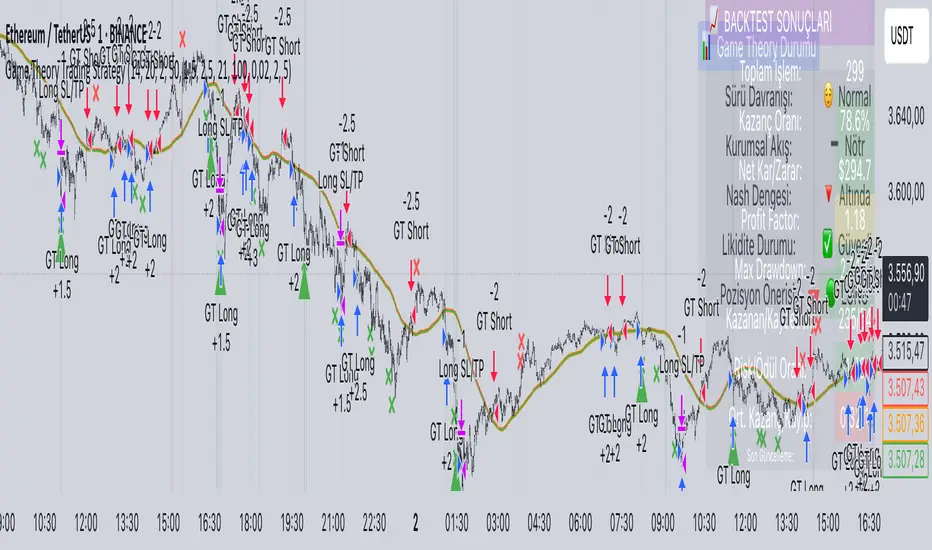
Game Theory Trading StrategyGame Theory Trading Strategy: Explanation and Working Logic
This Pine Script (version 5) code implements a trading strategy named "Game Theory Trading Strategy" in TradingView. Unlike the previous indicator, this is a full-fledged strategy with automated entry/exit rules, risk management, and backtesting capabilities. It uses Game Theory principles to analyze market behavior, focusing on herd behavior, institutional flows, liquidity traps, and Nash equilibrium to generate buy (long) and sell (short) signals. Below, I'll explain the strategy's purpose, working logic, key components, and usage tips in detail.
1. General Description
Purpose: The strategy identifies high-probability trading opportunities by combining Game Theory concepts (herd behavior, contrarian signals, Nash equilibrium) with technical analysis (RSI, volume, momentum). It aims to exploit market inefficiencies caused by retail herd behavior, institutional flows, and liquidity traps. The strategy is designed for automated trading with defined risk management (stop-loss/take-profit) and position sizing based on market conditions.
Key Features:
Herd Behavior Detection: Identifies retail panic buying/selling using RSI and volume spikes.
Liquidity Traps: Detects stop-loss hunting zones where price breaks recent highs/lows but reverses.
Institutional Flow Analysis: Tracks high-volume institutional activity via Accumulation/Distribution and volume spikes.
Nash Equilibrium: Uses statistical price bands to assess whether the market is in equilibrium or deviated (overbought/oversold).
Risk Management: Configurable stop-loss (SL) and take-profit (TP) percentages, dynamic position sizing based on Game Theory (minimax principle).
Visualization: Displays Nash bands, signals, background colors, and two tables (Game Theory status and backtest results).
Backtesting: Tracks performance metrics like win rate, profit factor, max drawdown, and Sharpe ratio.
Strategy Settings:
Initial capital: $10,000.
Pyramiding: Up to 3 positions.
Position size: 10% of equity (default_qty_value=10).
Configurable inputs for RSI, volume, liquidity, institutional flow, Nash equilibrium, and risk management.
Warning: This is a strategy, not just an indicator. It executes trades automatically in TradingView's Strategy Tester. Always backtest thoroughly and use proper risk management before live trading.
2. Working Logic (Step by Step)
The strategy processes each bar (candle) to generate signals, manage positions, and update performance metrics. Here's how it works:
a. Input Parameters
The inputs are grouped for clarity:
Herd Behavior (🐑):
RSI Period (14): For overbought/oversold detection.
Volume MA Period (20): To calculate average volume for spike detection.
Herd Threshold (2.0): Volume multiplier for detecting herd activity.
Liquidity Analysis (💧):
Liquidity Lookback (50): Bars to check for recent highs/lows.
Liquidity Sensitivity (1.5): Volume multiplier for trap detection.
Institutional Flow (🏦):
Institutional Volume Multiplier (2.5): For detecting large volume spikes.
Institutional MA Period (21): For Accumulation/Distribution smoothing.
Nash Equilibrium (⚖️):
Nash Period (100): For calculating price mean and standard deviation.
Nash Deviation (0.02): Multiplier for equilibrium bands.
Risk Management (🛡️):
Use Stop-Loss (true): Enables SL at 2% below/above entry price.
Use Take-Profit (true): Enables TP at 5% above/below entry price.
b. Herd Behavior Detection
RSI (14): Checks for extreme conditions:
Overbought: RSI > 70 (potential herd buying).
Oversold: RSI < 30 (potential herd selling).
Volume Spike: Volume > SMA(20) x 2.0 (herd_threshold).
Momentum: Price change over 10 bars (close - close ) compared to its SMA(20).
Herd Signals:
Herd Buying: RSI > 70 + volume spike + positive momentum = Retail buying frenzy (red background).
Herd Selling: RSI < 30 + volume spike + negative momentum = Retail selling panic (green background).
c. Liquidity Trap Detection
Recent Highs/Lows: Calculated over 50 bars (liquidity_lookback).
Psychological Levels: Nearest round numbers (e.g., $100, $110) as potential stop-loss zones.
Trap Conditions:
Up Trap: Price breaks recent high, closes below it, with a volume spike (volume > SMA x 1.5).
Down Trap: Price breaks recent low, closes above it, with a volume spike.
Visualization: Traps are marked with small red/green crosses above/below bars.
d. Institutional Flow Analysis
Volume Check: Volume > SMA(20) x 2.5 (inst_volume_mult) = Institutional activity.
Accumulation/Distribution (AD):
Formula: ((close - low) - (high - close)) / (high - low) * volume, cumulated over time.
Smoothed with SMA(21) (inst_ma_length).
Accumulation: AD > MA + high volume = Institutions buying.
Distribution: AD < MA + high volume = Institutions selling.
Smart Money Index: (close - open) / (high - low) * volume, smoothed with SMA(20). Positive = Smart money buying.
e. Nash Equilibrium
Calculation:
Price mean: SMA(100) (nash_period).
Standard deviation: stdev(100).
Upper Nash: Mean + StdDev x 0.02 (nash_deviation).
Lower Nash: Mean - StdDev x 0.02.
Conditions:
Near Equilibrium: Price between upper and lower Nash bands (stable market).
Above Nash: Price > upper band (overbought, sell potential).
Below Nash: Price < lower band (oversold, buy potential).
Visualization: Orange line (mean), red/green lines (upper/lower bands).
f. Game Theory Signals
The strategy generates three types of signals, combined into long/short triggers:
Contrarian Signals:
Buy: Herd selling + (accumulation or down trap) = Go against retail panic.
Sell: Herd buying + (distribution or up trap).
Momentum Signals:
Buy: Below Nash + positive smart money + no herd buying.
Sell: Above Nash + negative smart money + no herd selling.
Nash Reversion Signals:
Buy: Below Nash + rising close (close > close ) + volume > MA.
Sell: Above Nash + falling close + volume > MA.
Final Signals:
Long Signal: Contrarian buy OR momentum buy OR Nash reversion buy.
Short Signal: Contrarian sell OR momentum sell OR Nash reversion sell.
g. Position Management
Position Sizing (Minimax Principle):
Default: 1.0 (10% of equity).
In Nash equilibrium: Reduced to 0.5 (conservative).
During institutional volume: Increased to 1.5 (aggressive).
Entries:
Long: If long_signal is true and no existing long position (strategy.position_size <= 0).
Short: If short_signal is true and no existing short position (strategy.position_size >= 0).
Exits:
Stop-Loss: If use_sl=true, set at 2% below/above entry price.
Take-Profit: If use_tp=true, set at 5% above/below entry price.
Pyramiding: Up to 3 concurrent positions allowed.
h. Visualization
Nash Bands: Orange (mean), red (upper), green (lower).
Background Colors:
Herd buying: Red (90% transparency).
Herd selling: Green.
Institutional volume: Blue.
Signals:
Contrarian buy/sell: Green/red triangles below/above bars.
Liquidity traps: Red/green crosses above/below bars.
Tables:
Game Theory Table (Top-Right):
Herd Behavior: Buying frenzy, selling panic, or normal.
Institutional Flow: Accumulation, distribution, or neutral.
Nash Equilibrium: In equilibrium, above, or below.
Liquidity Status: Trap detected or safe.
Position Suggestion: Long (green), Short (red), or Wait (gray).
Backtest Table (Bottom-Right):
Total Trades: Number of closed trades.
Win Rate: Percentage of winning trades.
Net Profit/Loss: In USD, colored green/red.
Profit Factor: Gross profit / gross loss.
Max Drawdown: Peak-to-trough equity drop (%).
Win/Loss Trades: Number of winning/losing trades.
Risk/Reward Ratio: Simplified Sharpe ratio (returns / drawdown).
Avg Win/Loss Ratio: Average win per trade / average loss per trade.
Last Update: Current time.
i. Backtesting Metrics
Tracks:
Total trades, winning/losing trades.
Win rate (%).
Net profit ($).
Profit factor (gross profit / gross loss).
Max drawdown (%).
Simplified Sharpe ratio (returns / drawdown).
Average win/loss ratio.
Updates metrics on each closed trade.
Displays a label on the last bar with backtest period, total trades, win rate, and net profit.
j. Alerts
No explicit alertconditions defined, but you can add them for long_signal and short_signal (e.g., alertcondition(long_signal, "GT Long Entry", "Long Signal Detected!")).
Use TradingView's alert system with Strategy Tester outputs.
3. Usage Tips
Timeframe: Best for H1-D1 timeframes. Shorter frames (M1-M15) may produce noisy signals.
Settings:
Risk Management: Adjust sl_percent (e.g., 1% for volatile markets) and tp_percent (e.g., 3% for scalping).
Herd Threshold: Increase to 2.5 for stricter herd detection in choppy markets.
Liquidity Lookback: Reduce to 20 for faster markets (e.g., crypto).
Nash Period: Increase to 200 for longer-term analysis.
Backtesting:
Use TradingView's Strategy Tester to evaluate performance.
Check win rate (>50%), profit factor (>1.5), and max drawdown (<20%) for viability.
Test on different assets/timeframes to ensure robustness.
Live Trading:
Start with a demo account.
Combine with other indicators (e.g., EMAs, support/resistance) for confirmation.
Monitor liquidity traps and institutional flow for context.
Risk Management:
Always use SL/TP to limit losses.
Adjust position_size for risk tolerance (e.g., 5% of equity for conservative trading).
Avoid over-leveraging (pyramiding=3 can amplify risk).
Troubleshooting:
If no trades are executed, check signal conditions (e.g., lower herd_threshold or liquidity_sensitivity).
Ensure sufficient historical data for Nash and liquidity calculations.
If tables overlap, adjust position.top_right/bottom_right coordinates.
4. Key Differences from the Previous Indicator
Indicator vs. Strategy: The previous code was an indicator (VP + Game Theory Integrated Strategy) focused on visualization and alerts. This is a strategy with automated entries/exits and backtesting.
Volume Profile: Absent in this strategy, making it lighter but less focused on high-volume zones.
Wick Analysis: Not included here, unlike the previous indicator's heavy reliance on wick patterns.
Backtesting: This strategy includes detailed performance metrics and a backtest table, absent in the indicator.
Simpler Signals: Focuses on Game Theory signals (contrarian, momentum, Nash reversion) without the "Power/Ultra Power" hierarchy.
Risk Management: Explicit SL/TP and dynamic position sizing, not present in the indicator.
5. Conclusion
The "Game Theory Trading Strategy" is a sophisticated system leveraging herd behavior, institutional flows, liquidity traps, and Nash equilibrium to trade market inefficiencies. It’s designed for traders who understand Game Theory principles and want automated execution with robust risk management. However, it requires thorough backtesting and parameter optimization for specific markets (e.g., forex, crypto, stocks). The backtest table and visual aids make it easy to monitor performance, but always combine with other analysis tools and proper capital management.
If you need help with backtesting, adding alerts, or optimizing parameters, let me know!
TIME-SPLT ACADEMY INDICATOR# TIME-SPLT ACADEMY CISD + FVG + TSM FRACTALS - Comprehensive Market Structure Analysis Tool
## Overview
This indicator combines three essential market structure analysis components into a unified trading tool: Change in State Direction (CISD), Fair Value Gaps (FVG), and TSM Fractals. This integration provides traders with a complete framework for identifying market structure breaks, price imbalances, and key pivot levels on any timeframe.
## Component 1: CISD (Change in State Direction)
**What it is:** CISD identifies significant breaks in market structure by tracking when price decisively breaks above previous swing highs (bullish CISD) or below previous swing lows (bearish CISD). This concept is fundamental to understanding trend changes and continuation patterns.
**How it works:**
- Monitors swing highs and lows using customizable pivot periods
- Tracks when price closes above a previous swing high (bullish structure break)
- Tracks when price closes below a previous swing low (bearish structure break)
- Draws horizontal lines from the pivot point to the break point with "CISD" labels
- Works on multiple timeframes simultaneously
**Trading Applications:**
- Identifies trend changes and continuation signals
- Provides entry signals on structure breaks
- Helps determine market bias and direction
## Component 2: FVG (Fair Value Gaps)
**What it is:** Fair Value Gaps are price imbalances that occur when there's a gap between the high of one candle and the low of another candle two periods later, with the middle candle not filling this gap. These represent areas where price moved inefficiently and often return to "fill" the gap.
**How it works:**
- Analyzes 3-candle patterns to identify gaps
- Bearish FVG: Gap between low and high where price dropped leaving unfilled space above
- Bullish FVG: Gap between high and low where price rose leaving unfilled space below
- Tracks 8 different candle body combinations for each direction (up, down, doji patterns)
- Monitors gap mitigation when price returns to fill the imbalance
- Changes color when gaps are partially or fully mitigated
**Gap Detection Logic:**
- Bearish FVG patterns: DDD, DDJ, JDD, UDJ, JDU, UDD, DDU, UDU
- Bullish FVG patterns: DUD, DUJ, JUD, UUJ, JUU, UUD, DUU, UUU
- (D=Down candle, U=Up candle, J=Doji candle)
**Trading Applications:**
- High-probability reversal zones when price returns to FVGs
- Support and resistance levels
- Target areas for limit orders
- Risk management reference points
## Component 3: TSM Fractals
**What it is:** TSM Fractals identify significant pivot highs and lows using Williams Fractal methodology. These mark potential reversal points and key support/resistance levels.
**How it works:**
- Identifies fractal highs: peaks where the center candle's high is higher than surrounding candles
- Identifies fractal lows: valleys where the center candle's low is lower than surrounding candles
- Uses customizable lookback periods (default 15) for fractal identification
- Displays horizontal lines with "$" symbols at fractal levels
- Maintains a configurable number of recent fractals on the chart
**Trading Applications:**
- Key support and resistance levels
- Potential reversal zones
- Confluence with other analysis tools
- Stop loss placement reference points
## Why This Combination Works
**Synergistic Analysis:** Each component provides different but complementary information:
1. **CISD** shows when market structure changes, indicating trend shifts or continuation
2. **FVGs** reveal where price has moved inefficiently and may return for rebalancing
3. **Fractals** highlight key pivot points that often act as support/resistance
**Trading Edge:** The combination allows for:
- **Entry Confirmation:** Wait for CISD breaks near unfilled FVGs at fractal levels
- **Risk Management:** Use FVG boundaries and fractal levels for stop placement
- **Target Selection:** Project moves to opposite FVGs or fractal levels
- **Market Context:** Understand whether you're trading with or against structure
## Key Features
**Multi-Timeframe CISD:**
- Customizable timeframe settings (Minute, Hour, Day, Week, Month)
- Adjustable swing length for pivot identification
- Customizable line styles, widths, and colors
- Optional alerts on structure breaks
**Advanced FVG Management:**
- Automatic gap size filtering
- Real-time mitigation tracking
- Color-coded active vs. mitigated gaps
- Optional pip value labels
- Large gap alerts for significant imbalances
**Intelligent Fractal Display:**
- Configurable fractal periods
- Maximum fractal count management
- Clean visual presentation
- Historical fractal preservation
## Settings & Customization
**CISD Settings:**
- Timeframe selection and multipliers
- Swing length adjustment (default 7)
- Line styling options
- Color customization for bullish/bearish breaks
- Alert toggle options
**FVG Settings:**
- Show/hide toggles for each direction
- Minimum gap size filtering
- Alert threshold for large gaps
- Color schemes for active and mitigated gaps
- Optional size labels in pips
**Fractal Settings:**
- Fractal period adjustment (default 15)
- Maximum display count (default 10)
- Show/hide toggle
## Educational Value
This indicator teaches traders to:
- Understand market structure concepts
- Recognize price inefficiencies
- Identify key pivot points
- Combine multiple analysis methods
- Develop systematic trading approaches
## Use Cases
**Swing Trading:** Identify major structure breaks with FVG confluence
**Day Trading:** Use lower timeframe CISDs with intraday FVGs
**Scalping:** Quick entries at FVG mitigation near fractal levels
**Position Trading:** Higher timeframe structure analysis with major FVGs
## Technical Implementation
- Utilizes Pine Script v6 for optimal performance
- Efficient array management for historical data
- Real-time calculations without repainting
- Memory-optimized box and line management
- Multi-timeframe data handling with proper security functions
This comprehensive tool eliminates the need for multiple separate indicators, providing everything needed for complete market structure analysis in one cohesive package. The educational component helps traders understand not just what the signals are, but why they work and how to use them effectively in different market conditions.

Kijun Shifting Band Oscillator | QuantMAC🎯 Kijun Shifting Band Oscillator | QuantMAC
📊 **Revolutionary Technical Analysis Tool Combining Ancient Ichimoku Wisdom with Cutting-Edge Statistical Methods**
🌟 Overview
The Kijun Shifting Band Oscillator represents a sophisticated fusion of traditional Japanese technical analysis and modern statistical theory. Built upon the foundational concepts of the Ichimoku Kinko Hyo system, this indicator transforms the classic Kijun-sen (base line) into a dynamic, multi-dimensional analysis tool that provides traders with unprecedented market insights.
This advanced oscillator doesn't just show you where price has been – it reveals the underlying momentum dynamics and volatility patterns that drive market movements, giving you a statistical edge in your trading decisions.
🔥 Key Features & Innovations
Dual Trading Modes for Maximum Flexibility: 🚀
Long/Short Mode: Full bidirectional trading capability for aggressive traders seeking to capitalize on both bullish and bearish market conditions
Long/Cash Mode: Conservative approach perfect for risk-averse traders, taking long positions during uptrends and moving to cash during downtrends (avoiding short exposure)
Advanced Visual Intelligence: 🎨
9 Professional Color Schemes: From classic blue/navy to vibrant orange/purple combinations, each optimized for different chart backgrounds and personal preferences
Dynamic Gradient Histogram: Color intensity reflects oscillator strength, providing instant visual feedback on momentum magnitude
Intelligent Overlay Bands: Semi-transparent fills create clear visual boundaries without cluttering your chart
Smart Candle Coloring: Real-time color changes reflect current market state and trend direction
Customizable Threshold Lines: Clearly marked entry and exit levels with contrasting colors
Professional-Grade Analytics: 📊
Real-Time Performance Metrics: Live calculation of 9 key performance indicators
Risk-Adjusted Returns: Sharpe, Sortino, and Omega ratios for comprehensive performance evaluation
Position Sizing Guidance: Half-Kelly percentage for optimal risk management
Drawdown Analysis: Maximum drawdown tracking for risk assessment
📈 Deep Technical Foundation
Kijun-Based Mathematical Framework: 🧮
The indicator begins with the traditional Kijun-sen calculation but extends it significantly:
Statistical Enhancements: 📉
Adaptive Volatility: Bands expand and contract based on market volatility
Momentum Filtering: EMA smoothing of oscillator for trend confirmation
State Management: Intelligent signal filtering prevents whipsaws and false signals
Multi-Timeframe Compatibility: Optimized algorithms work across all timeframes
⚙️ Comprehensive Parameter Control
Kijun Core Settings: 🎛️
Kijun Length (Default: 30): Controls the lookback period for the base calculation. Shorter periods = more responsive, longer periods = smoother signals
Source Selection: Choose from Close, Open, High, Low, or HL2. Close price recommended for most applications
Calculation Method: Uses traditional Ichimoku methodology ensuring compatibility with classic analysis
Advanced Oscillator Configuration: 📊
Standard Deviation Length (Default: 36): Determines volatility measurement period. Affects band width and sensitivity
SD Multiplier (Default: 2.1): Fine-tune band distance from basis line. Higher values = wider bands, lower values = tighter bands
Oscillator Multiplier (Default: 100): Scales the final oscillator output. Useful for matching other indicators or personal preference
Smoothing Algorithm: Built-in EMA smoothing prevents noise while maintaining responsiveness
Signal Threshold Optimization: 🎯
Long Threshold (Default: 83): Oscillator level that triggers long entries. Higher values = fewer but stronger signals
Short Threshold (Default: 42): Oscillator level that triggers short entries. Lower values = fewer but stronger signals
Threshold Logic: Crossover-based system with state management prevents signal overlap
Customization Range: Fully adjustable to match your trading style and risk tolerance
Precision Date Control: 📅
Start Date/Month/Year: Precise backtesting control down to the day
Historical Analysis: Test strategies on specific market periods or events
Strategy Validation: Isolate performance during different market conditions
📊 Professional Metrics Dashboard
Risk Assessment Metrics: 💼
Maximum Drawdown %: Largest peak-to-trough decline in portfolio value. Critical for understanding worst-case scenarios and position sizing
Sortino Ratio: Risk-adjusted return measure focusing only on downside volatility. Superior to Sharpe ratio for asymmetric return distributions
Sharpe Ratio: Classic risk-adjusted performance metric. Values above 1.0 considered good, above 2.0 excellent
Omega Ratio: Probability-weighted ratio capturing all moments of return distribution. More comprehensive than Sharpe or Sortino
Performance Analytics: 📈
Profit Factor: Gross Profit ÷ Gross Loss. Values above 1.0 indicate profitability, above 2.0 considered excellent
Win Rate %: Percentage of profitable trades. Consider alongside average win/loss size for complete picture
Net Profit %: Total return on initial capital. Accounts for compounding effects
Total Trades: Sample size for statistical significance assessment
Advanced Position Sizing: 🎯
Half Kelly %: Optimal position size based on Kelly Criterion, reduced by 50% for safety margin
Risk Management: Helps determine appropriate position size relative to account equity
Mathematical Foundation: Based on win probability and profit factor calculations
Practical Application: Directly usable percentage for position sizing decisions
🎨 Advanced Display Options
Flexible Interface Design: 🖥️
6 Positioning Options: Top/Bottom/Middle × Left/Right combinations for optimal chart organization
Toggle Functionality: Show/hide metrics table for clean chart presentation during analysis
Color Coordination: Metrics table colors match selected oscillator color scheme
Professional Styling: Clean, readable format with proper spacing and alignment
Visual Hierarchy: 🎭
Oscillator Histogram: Primary focus with gradient intensity showing momentum strength
Threshold Lines: Clear horizontal references for entry/exit levels
Zero Line: Neutral reference point for trend bias determination
Background Bands: Subtle overlay context without chart clutter
🚀 Advanced Signal Generation System
Multi-Layer Signal Logic: ⚡
Primary Signal Generation: Oscillator crossover above Long Threshold (default 83) triggers long entries
Exit Signal Processing: Oscillator crossunder below Short Threshold (default 42) triggers position exits
State Management System: Prevents duplicate signals and ensures clean position transitions
Mode-Specific Logic: Different behavior for Long/Short vs Long/Cash modes
Date Range Filtering: Signals only generated within specified backtesting period
Confirmation Requirements: Bar confirmation prevents false signals from intrabar price spikes
Intelligent Position Management: 🧠
Entry Tracking: Precise entry price recording for accurate P&L calculations
Position State Monitoring: Continuous tracking of long/short/cash positions
Automatic Exit Logic: Seamless position closure and new position initiation
Performance Calculation: Real-time P&L tracking with compounding effects
📉📈 Comprehensive Band Interpretation Guide
Dynamic Band Analysis: 🔍
Upper Band Function: Represents dynamic resistance based on recent volatility. Price approaching upper band suggests potential reversal or breakout
Lower Band Function: Represents dynamic support with volatility adjustment. Price near lower band indicates oversold conditions or support testing
Middle Line (Basis): Trend direction indicator. Price above = bullish bias, price below = bearish bias
Band Width Interpretation: Wide bands = high volatility, narrow bands = low volatility/potential breakout setup
Band Slope Analysis: Rising bands = strengthening trend, falling bands = weakening trend
Oscillator Interpretation: 📊
Values Above 50: Price in upper half of recent range, bullish momentum
Values Below 50: Price in lower half of recent range, bearish momentum
Extreme Values (>80 or <20): Overbought/oversold conditions, potential reversal zones
Momentum Divergence: Oscillator direction vs price direction for early reversal signals
Trend Confirmation: Oscillator direction confirming or contradicting price trends
💡 Strategic Trading Applications
Primary Trading Strategies: 🎯
Trend Following: Use threshold crossovers to capture major directional moves. Best in trending markets with clear directional bias
Mean Reversion: Identify extreme oscillator readings for counter-trend opportunities. Effective in range-bound markets
Breakout Trading: Monitor band compressions followed by expansions for breakout signals
Swing Trading: Combine oscillator signals with band interactions for swing position entries/exits
Risk Management: Use metrics dashboard for position sizing and risk assessment
Market Condition Optimization: 🌊
Trending Markets: Increase threshold separation for fewer, stronger signals
Choppy Markets: Decrease threshold separation for more responsive signals
High Volatility: Increase SD multiplier for wider bands
Low Volatility: Decrease SD multiplier for tighter bands and earlier signals
⚙️ Advanced Configuration Tips
Parameter Optimization Guidelines: 🔧
Kijun Length Adjustment: Shorter periods (10-20) for faster signals, longer periods (50-100) for smoother trends
SD Length Tuning: Match to your trading timeframe - shorter for responsive, longer for stability
Threshold Calibration: Backtest different levels to find optimal entry/exit points for your market
Color Scheme Selection: Choose schemes that provide best contrast with your chart background and other indicators
Integration with Other Indicators: 🔗
Volume Indicators: Confirm oscillator signals with volume spikes
Support/Resistance: Use key levels to filter oscillator signals
Momentum Indicators: RSI, MACD confirmation for signal strength
Trend Indicators: Moving averages for overall trend bias confirmation
⚠️ Important Usage Notes & Limitations
Indicator Characteristics: ⚡
Lagging Nature: Based on historical price data - signals occur after moves have begun
Best Practice: Combine with leading indicators and price action analysis
Market Dependency: Performance varies across different market conditions and instruments
Backtesting Essential: Always validate parameters on historical data before live implementation
Optimization Recommendations: 🎯
Parameter Testing: Systematically test different combinations on your preferred instruments
Walk-Forward Analysis: Regularly re-optimize parameters to maintain effectiveness
Market Regime Awareness: Adjust parameters for different market conditions (trending vs ranging)
Risk Controls: Implement maximum drawdown limits and position size controls
🔧 Technical Specifications
Performance Optimization: ⚡
Efficient Algorithms: Optimized calculations for smooth real-time operation
Memory Management: Smart array handling for metrics calculations
Visual Optimization: Balanced detail vs performance for responsive charts
Multi-Symbol Ready: Consistent performance across different assets
---
The Kijun Shifting Band Oscillator represents the evolution of technical analysis, bridging the gap between traditional methods and modern quantitative approaches. This indicator provides traders with a comprehensive toolkit for market analysis, combining the intuitive wisdom of Japanese candlestick analysis with the precision of statistical mathematics.
🎯 Designed for serious traders who demand professional-grade analysis tools with institutional-quality metrics and risk management capabilities. Whether you're a discretionary trader seeking visual confirmation or a systematic trader building quantitative strategies, this indicator provides the foundation for informed trading decisions.
⚠️ IMPORTANT DISCLAIMER
Past Performance Warning: 📉⚠️
PAST PERFORMANCE IS NOT INDICATIVE OF FUTURE RESULTS. Historical backtesting results, while useful for strategy development and parameter optimization, do not guarantee similar performance in live trading conditions. Market conditions change continuously, and what worked in the past may not work in the future.
Remember: Successful trading requires discipline, continuous learning, and adaptation to changing market conditions. No indicator or strategy guarantees profits, and all trading involves substantial risk of loss.

Machine Learning | Adaptive Trend Signals [Bitwardex]⚙️🧠Machine Learning | Adaptive Trend Signals
🔷Overview
Machine Learning | Adaptive Trend Signals is a Pine Script™ v6 indicator designed to visualize market trends and generate signals through a combination of volatility clustering, Gaussian smoothing, and adaptive trend calculations. Built as an overlay indicator, it integrates advanced techniques inspired by machine learning concepts, such as K-Means clustering, to adapt to changing market conditions. The script is highly customizable, includes a backtesting module, and supports alert conditions, making it suitable for traders exploring trend-based strategies and developers studying volatility-driven indicator design.
🔷Functionality
The indicator performs the following core functions:
• Volatility Clustering: Uses K-Means clustering to categorize market volatility into high, medium, and low states, adjusting trend sensitivity accordingly.
• Trend Calculation: Computes adaptive trend lines (SmartTrend) based on volatility-adjusted standard deviation, smoothed RSI, and ADX filters.
• Signal Generation: Identifies potential buy and sell points through trend line crossovers and directional confirmation.
• Backtesting Module: Tracks trade outcomes based on the SmartTrend3 value, displaying win rate and total trades.
• Visualization: Plots trend lines with gradient colors and optional signal markers (bullish 🐮 and bearish 🐻).
• Alerts: Provides configurable alerts for trend shifts and volatility state changes.
🔷Technical Methodology
Volatility Clustering with K-Means
The indicator employs a K-Means clustering algorithm to classify market volatility, measured via the Average True Range (ATR), into three distinct clusters:
• Data Collection: Gathers ATR values over a user-defined training period (default: 100 bars).
• Centroid Initialization: Sets initial centroids at the highest, lowest, and midpoint ATR values within the training period.
• Iterative Clustering: Assigns ATR data points to the nearest centroid, recalculates centroid means, and repeats until convergence.
• Dynamic Adjustment: Assigns a volatility state (high, medium, or low) based on the closest centroid, adjusting the trend factor (e.g., tighter for high volatility, wider for low volatility).
This approach allows the indicator to adapt its sensitivity to varying market conditions, providing a data-driven foundation for trend calculations.
🔷Gaussian Smoothing
To enhance signal clarity and reduce noise, the indicator applies Gaussian kernel smoothing to:
• RSI: Smooths the Relative Strength Index (calculated from OHLC4) to filter short-term fluctuations.
• SmartTrend: Smooths the primary trend line for a more stable output.
The Gaussian kernel uses a sigma value derived from the user-defined smoothing length, ensuring mathematically consistent noise reduction.
🔷SmartTrend Calculation
The pineSmartTrend function is the core of the indicator, producing three trend lines:
• SmartTrend: The primary trend line, calculated using a volatility-adjusted standard deviation, smoothed RSI, and ADX conditions.
• SmartTrend2: A secondary trend line with a wider factor (base factor * 1.382) for signal confirmation.
SmartTrend3: The average of SmartTrend and SmartTrend2, used for plotting and backtesting.
Key components of the calculation include:
• Dynamic Standard Deviation: Scales based on ATR relative to its 50-period smoothed average, with multipliers (1.0 to 1.4) applied according to volatility thresholds.
• RSI and ADX Filters: Requires RSI > 50 for bullish trends or < 50 for bearish trends, alongside ADX > 15 and rising to confirm trend strength.
Volatility-Adjusted Bands: Constructs upper and lower bands around price action, adjusted by the volatility cluster’s dynamic factor.
🔷Signal Generation
The generate_signals function generates signals as follows:
• Buy Signal: Triggered when SmartTrend crosses above SmartTrend2 and the price is above SmartTrend, with directional confirmation.
• Sell Signal: Triggered when SmartTrend crosses below SmartTrend2 and the price is below SmartTrend, with directional confirmation.
Directional Logic: Tracks trend direction to filter out conflicting signals, ensuring alignment with the broader market context.
Signals are visualized as small circles with bullish (🐮) or bearish (🐻) emojis, with an option to toggle visibility.
🔷Backtesting
The get_backtest function evaluates signal outcomes using the SmartTrend3 value (rather than closing prices) to align with the trend-based methodology.
It tracks:
• Total Trades: Counts completed long and short trades.
• Win Rate: Calculates the percentage of trades where SmartTrend3 moves favorably (higher for longs, lower for shorts).
Position Management: Closes opposite positions before opening new ones, simulating a single-position trading system.
Results are displayed in a table at the top-right of the chart, showing win rate and total trades. Note that backtest results reflect the indicator’s internal logic and should not be interpreted as predictive of real-world performance.
🔷Visualization and Alerts
• Trend Lines: SmartTrend3 is plotted with gradient colors reflecting trend direction and volatility cluster, accompanied by a secondary line for visual clarity.
• Signal Markers: Optional buy/sell signals are plotted as small circles with customizable colors.
• Alerts: Supports alerts for:
• Bullish and bearish trend shifts (confirmed on bar close).
Transitions to high, medium, or low volatility states.
🔷Input Parameters
• ATR Length (default: 14): Period for ATR calculation, used in volatility clustering.
• Period (default: 21): Common period for RSI, ADX, and standard deviation calculations.
• Base SmartTrend Factor (default: 2.0): Base multiplier for volatility-adjusted bands.
• SmartTrend Smoothing Length (default: 10): Length for Gaussian smoothing of the trend line.
• Show Buy/Sell Signals? (default: true): Enables/disables signal markers.
• Bullish/Bearish Color: Customizable colors for trend lines and signals.
🔷Usage Instructions
• Apply to Chart: Add the indicator to any TradingView chart.
• Configure Inputs: Adjust parameters to align with your trading style or market conditions (e.g., shorter ATR length for faster markets).
• Interpret Output:
• Trend Lines: Use SmartTrend3’s direction and color to gauge market bias.
• Signals: Monitor bullish (🐮) and bearish (🐻) markers for potential entry/exit points.
• Backtest Table: Review win rate and total trades to understand the indicator’s behavior in historical data.
• Set Alerts: Configure alerts for trend shifts or volatility changes to support manual or automated trading workflows.
• Combine with Analysis: Use the indicator alongside other tools or market context, as it is designed to complement, not replace, comprehensive analysis.
🔷Technical Notes
• Data Requirements: Requires at least 100 bars for accurate volatility clustering. Ensure sufficient historical data is loaded.
• Market Suitability: The indicator is designed for trend detection and may perform differently in ranging or volatile markets due to its reliance on RSI and ADX filters.
• Backtesting Scope: The backtest module uses SmartTrend3 values, which may differ from price-based outcomes. Results are for informational purposes only.
• Computational Intensity: The K-Means clustering and Gaussian smoothing may increase processing time on lower timeframes or with large datasets.
🔷For Developers
The script is modular, well-commented, encouraging reuse and modification with proper attribution.
Key functions include:
• gaussianSmooth: Applies Gaussian kernel smoothing to any data series.
• pineSmartTrend: Computes adaptive trend lines with volatility and momentum filters.
• getDynamicFactor: Adjusts trend sensitivity based on volatility clusters.
• get_backtest: Evaluates signal performance using SmartTrend3.
Developers can extend these functions for custom indicators or strategies, leveraging the volatility clustering and smoothing methodologies. The K-Means implementation is particularly useful for adaptive volatility analysis.
🔷Limitations
• The indicator is not predictive and should be used as part of a broader trading strategy.
• Performance varies by market, timeframe, and parameter settings, requiring user experimentation.
• Backtest results are based on historical data and internal logic, not real-world trading conditions.
• Volatility clustering assumes sufficient historical data; incomplete data may affect accuracy.
🔷Acknowledgments
Developed by Bitwardex, inspired by machine learning concepts and adaptive trading methodologies. Community feedback is welcome via TradingView’s platform.
🔷 Risk Disclaimer
Trading involves significant risks, and most traders may incur losses. Bitwardex AI Algo is provided for informational and educational purposes only and does not constitute financial advice or a recommendation to buy or sell any financial instrument . The signals, metrics, and features are tools for analysis and do not guarantee profits or specific outcomes. Past performance is not indicative of future results. Always conduct your own due diligence and consult a financial advisor before making trading decisions.

Volume Profile & Smart Money Explorer🔍 Volume Profile & Smart Money Explorer: Decode Institutional Footprints
Master the art of institutional trading with this sophisticated volume analysis tool. Track smart money movements, identify peak liquidity windows, and align your trades with major market participants.
🌟 Key Features:
📊 Triple-Layer Volume Analysis
• Total Volume Patterns
• Directional Volume Split (Up/Down)
• Institutional Flow Detection
• Real-time Smart Money Tracking
• Historical Pattern Recognition
⚡ Smart Money Detection
• Institutional Trade Identification
• Large Block Order Tracking
• Smart Money Concentration Periods
• Whale Activity Alerts
• Volume Threshold Analysis
📈 Advanced Profiling
• Hourly Volume Distribution
• Directional Bias Analysis
• Liquidity Heat Maps
• Volume Pattern Recognition
• Custom Threshold Settings
🎯 Strategic Applications:
Institutional Trading:
• Track Big Player Movements
• Identify Accumulation/Distribution
• Follow Smart Money Flow
• Detect Institutional Trading Windows
• Monitor Block Orders
Risk Management:
• Identify High Liquidity Windows
• Avoid Thin Market Periods
• Optimize Position Sizing
• Track Market Participation
• Monitor Volume Quality
Market Analysis:
• Volume Pattern Recognition
• Smart Money Flow Analysis
• Liquidity Window Identification
• Institutional Activity Cycles
• Market Depth Analysis
💡 Perfect For:
• Professional Traders
• Volume Profile Traders
• Institutional Traders
• Risk Managers
• Algorithmic Traders
• Smart Money Followers
• Day Traders
• Swing Traders
📊 Key Metrics:
• Normalized Volume Profiles
• Institutional Thresholds
• Directional Volume Split
• Smart Money Concentration
• Historical Patterns
• Real-time Analysis
⚡ Trading Edge:
• Trade with Institution Flow
• Identify Optimal Entry Points
• Recognize Distribution Patterns
• Follow Smart Money Positioning
• Avoid Thin Markets
• Capitalize on Peak Liquidity
🎓 Educational Value:
• Understand Market Structure
• Learn Volume Analysis
• Master Institutional Patterns
• Develop Market Intuition
• Track Smart Money Flow
🛠️ Customization:
• Adjustable Time Windows
• Flexible Volume Thresholds
• Multiple Timeframe Analysis
• Custom Alert Settings
• Visual Preference Options
Whether you're tracking institutional flows in crypto markets or following smart money in traditional markets, the Volume Profile & Smart Money Explorer provides the deep insights needed to trade alongside the biggest players.
Transform your trading from retail guesswork to institutional precision. Know exactly when and where smart money moves, and position yourself ahead of major market shifts.
#VolumeProfile #SmartMoney #InstitutionalTrading #MarketAnalysis #TradingView #VolumeAnalysis #CryptoTrading #ForexTrading #TechnicalAnalysis #Trading #PriceAction #MarketStructure #OrderFlow #Liquidity #RiskManagement #TradingStrategy #DayTrading #SwingTrading #AlgoTrading #QuantitativeTrading
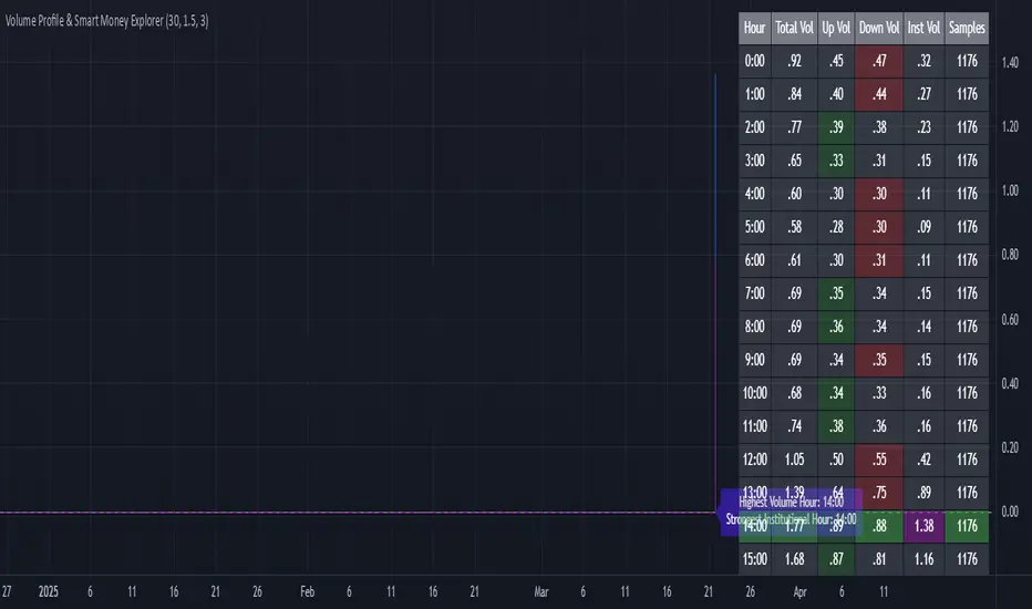
X Levels [Pro+] (TradeX)Introduction:
The X-Levels Indicator is a cutting-edge trading tool to help identify key price levels around Premium / Discount Arrays (PD arrays) at Higher Timeframe Points of Interest. It aids the trader by automatically measuring dealing ranges across multiple Timeframes and highlighting the percentages within which define a Premium & Discount Range. These percentages, known as X-Levels, are where the trader seeks an entry around a relevant PD array. This approach allows a trader to optimize entry and exit points around X-Levels. Suitable for traders of all levels, X-Levels enhances analysts' trade location and framework, providing crucial insights into market movements.
What is an X-Level? A specific percentage within any given dealing range that defines a premium and discount. X Levels are defined as the following percents: 0,12,21,29.5,38,50,61.8,70.5,79,88,100. Percentages below 50% indicate a discount and above 50% indicate a premium.
Foundation: This methodology, developed by TradeX, defines a consistent way for defining dealing ranges and his key percentage levels. Built upon Inner Circle Trader (ICT)’s principles of price delivery, it recognizes that price moves between premium and discount levels, seeking liquidity and inefficiencies.
After extensive refinements, this tool now automates the identification of these dealing ranges across any Timeframe, whilst presenting the X-Levels in a clear and precise manner allowing traders to track price movements with precision and efficiency across multiple time frames.
As price moves between X-Levels, it is the trader’s role to analyze which PD Array offers the best entry opportunity around a given X-Level. The true value of this tool lies in its ability to automatically update Dealing Ranges in real Time, eliminating the need for manual measurement or adjustment. This not only saves Time but also allows analysts to focus on trading rather than manually drawing and updating dealing ranges, removing guess work from defining the correct X Levels dealing range.
When X-Levels are applied across multiple Timeframes, traders gain a comprehensive view of the current market conditions. A key principle of this approach is aligning with price at Higher Timeframe (HTF) Point of Interest. By tracking dealing ranges from HTF while operating in Lower Timeframes, analysts can maintain a granular view while keeping track of the HTF framework.
Explanation of Killzones
Killzones refer to the times when major financial markets are open and active, particularly the London and New York sessions. For example, the London Open Killzone typically runs from 2:00 AM to 4:00 AM Eastern Time, while the New York Killzone is often from 8:00 AM to 10:00 AM Eastern Time. During these times, traders can expect more significant price movements due to higher trading volumes and the overlap of market participants.
The X-Levels indicator includes customizable killzone delineations, allowing traders to tailor this setting to their preferred trading sessions.
Key Opening Prices
Finally, the X-Levels indicator also includes Opening Price Delineations in both Horizontal and Vertical delineation. The "opening price" in trading refers to the first price at which a security is traded when the market opens. This price is significant because it can set the tone for the day's trading and is often used as a reference point for analyzing market movements. We are tracking midnight open, 8:30am and 9:30am. This is due to Midnight Theory.
Midnight Theory:
This is following the principles of Power of 3 (PO3) where if a trader is seeking a bullish expansion on a daily candle he is looking to frame entries below the midnight opening price. The principle of midnight theory comes in the form of buying at a hypothetical discount. A trade entering below midnight would be considered a discount, below midnight and 9:30am on a bullish day would be considered a deep discount.
Settings Summary:
Dealing Ranges: Traders can choose which Timeframe to track and can choose up to a maximum of 3 per chart. The styles of which are fully customizable. Solid lines, dotted lines or dashed lines are all available options for presenting each X-Level on each Dealing Range.
Dealing Range Labels: Above and below each Dealing Range extreme, analysts can find a label marking what Timeframe it originates from to differentiate between multiple Dealing Ranges. The size of this label can be hidden, and if shown its size can be customized.
Customizable Colors: Each Dealing Range Discount, Fair Value, and Premium, can be customized at the choice of the trader to suit their preferences.
Manual Dealing Range: If a trader would like to manually set their own Dealing Range, they can do so by marking the beginning of the Dealing Range view window visually through a tailored Manual Dealing Range setting.
Table Presentation: A table that can be presented in different locations on the chart, showing the percentages in relation to where price is trading in any given active Dealing Range. This is an incredibly useful tool for those wanting to see where they sit across Timeframes quickly.
Killzone Delineations: Traders can customize the Times of their preferred Killzones, whether conventional sessions, or their own preference. Their individual colors can also be customized to the trader's liking and preference.
Opening Prices: Traders can customize the colours to suit preferences and change the line thickness, plus adjust and label size.
Conclusion
The X-Levels Indicator is a powerful tool designed to streamline and enhance a trader’s ability to identify key price levels, track Dealing Ranges automatically, and highlight opportunities around Premium and Discount. By automating the measurement of dealing ranges and dynamically updating X-Levels across multiple Timeframes, this indicator eliminates the need for manual calculations, saving Time and allowing traders to focus on narrative.
When combined with Killzone delineations and Opening Prices, the indicator provides a comprehensive framework for aligning trades within the broader market context.
Whether used by beginners or experienced traders, the X-Levels Indicator empowers market participants with a structured approach to price action, liquidity dynamics, and trade location.
Usage Guidance:
Add X Levels° (TradeX) to your TradingView chart.
Select your preferred Timeframes for Dealing Ranges, Killzones, and Opening Prices.
Automate your analysis process with X Levels° (TradeX) and leverage it into your existing strategies to fine-tune your view through automatic Dealing Range tracking and charting.
Terms and Conditions
Our charting tools are products provided for informational and educational purposes only and do not constitute financial, investment, or trading advice. Our charting tools are not designed to predict market movements or provide specific recommendations. Users should be aware that past performance is not indicative of future results and should not be relied upon for making financial decisions. By using our charting tools, the purchaser agrees that the seller and the creator are not responsible for any decisions made based on the information provided by these charting tools. The purchaser assumes full responsibility and liability for any actions taken and the consequences thereof, including any loss of money or investments that may occur as a result of using these products. Hence, by purchasing these charting tools, the customer accepts and acknowledges that the seller and the creator are not liable nor responsible for any unwanted outcome that arises from the development, the sale, or the use of these products. Finally, the purchaser indemnifies the seller from any and all liability. If the purchaser was invited through the Friends and Family Program, they acknowledge that the provided discount code only applies to the first initial purchase of the Toodegrees Premium Suite subscription. The purchaser is therefore responsible for cancelling – or requesting to cancel – their subscription in the event that they do not wish to continue using the product at full retail price. If the purchaser no longer wishes to use the products, they must unsubscribe from the membership service, if applicable. We hold no reimbursement, refund, or chargeback policy. Once these Terms and Conditions are accepted by the Customer, before purchase, no reimbursements, refunds or chargebacks will be provided under any circumstances.
By continuing to use these charting tools, the user acknowledges and agrees to the Terms and Conditions outlined in this legal disclaimer.

AMD Session Structure Levels# Market Structure & Manipulation Probability Indicator
## Overview
This advanced indicator is designed for traders who want a systematic approach to analyzing market structure, identifying manipulation, and assessing probability-based trade setups. It incorporates four core components:
### 1. Session Price Action Analysis
- Tracks **OHLC (Open, High, Low, Close)** within defined sessions.
- Implements a **dual tracking system**:
- **Official session levels** (fixed from the session open to close).
- **Real-time max/min tracking** to differentiate between temporary spikes and real price acceptance.
### 2. Market Manipulation Detection
- Identifies **manipulative price action** using the relationship between the open and close:
- If **price closes below open** → assumes **upward manipulation**, followed by **downward distribution**.
- If **price closes above open** → assumes **downward manipulation**, followed by **upward distribution**.
- Normalized using **ATR**, ensuring adaptability across different volatility conditions.
### 3. Probability Engine
- Tracks **historical wick ratios** to assess trend vs. reversal conditions.
- Calculates **conditional probabilities** for price moves.
- Uses a **special threshold system (0.45 and 0.03)** for reversal signals.
- Provides **real-time probability updates** to enhance trade decision-making.
### 4. Market Condition Classification
- Classifies market conditions using a **wick-to-body ratio**:
```pine
wick_to_body_ratio = open > close ? upper_wick / (high - low) : lower_wick / (high - low)
```
- **Low ratio (<0.25)** → Likely a **trend day**.
- **High ratio (>0.25)** → Likely a **range day**.
---
## Why This Indicator Stands Out
### ✅ Smarter Level Detection
- Uses **ATR-based dynamic levels** instead of static support/resistance.
- Differentiates **manipulation from distribution** for better decision-making.
- Updates probabilities **in real-time**.
### ✅ Memory-Efficient Design
- Implements **circular buffers** to maintain efficiency:
```pine
var float manipUp = array.new_float(lookbackPeriod, 0.0)
var float manipDown = array.new_float(lookbackPeriod, 0.0)
```
- Ensures **constant memory usage**, even over extended trading sessions.
### ✅ Advanced Probability Calculation
- Utilizes **conditional probabilities** instead of simple averages.
- Incorporates **market context** through wick analysis.
- Provides **actionable signals** via a probability table.
---
## Trading Strategy Guide
### **Best Entry Setups**
✅ Wait for **price to approach manipulation levels**.
✅ Confirm using the **probability table**.
✅ Check the **wick ratio for context**.
✅ Enter when **conditional probability aligns**.
### **Smart Exit Management**
✅ Use **distribution levels** as **profit targets**.
✅ Scale out **when probabilities shift**.
✅ Monitor **wick percentiles** for confirmation.
### **Risk Management**
✅ Size positions based on **probability readings**.
✅ Place stops at **manipulation levels**.
✅ Adjust position size based on **trend vs. range classification**.
---
## Configuration Tips
### **Session Settings**
```pine
sessionTime = input.session("0830-1500", "Session Hours")
weekDays = input.string("23456", "Active Days")
```
- Match these to your **primary trading session**.
- Adjust for different **market opens** if needed.
### **Analysis Parameters**
```pine
lookbackPeriod = input.int(50, "Lookback Period")
low_threshold = input.float(0.25, "Trend/Range Threshold")
```
- **50 periods** is a good starting point but can be optimized per instrument.
- The **0.25 threshold** is ideal for most markets but may need adjustments.
---
## Market Structure Breakdown
### **Trend/Continuation Days**
- **Characteristics:**
✅ Small **opposing wicks** (minimal counter-pressure).
✅ Clean, **directional price movement**.
- **Bullish Trend Day Example:**
✅ Small **lower wicks** (minimal downward pressure).
✅ Strong **closes near the highs** → **Buyers in control**.
- **Bearish Trend Day Example:**
✅ Small **upper wicks** (minimal upward pressure).
✅ Strong **closes near the lows** → **Sellers in control**.
### **Reversal Days**
- **Characteristics:**
✅ **Large opposing wicks** → Failed momentum in the initial direction.
- **Bullish Reversal Example:**
✅ **Large upper wick early**.
✅ **Strong close from the lows** → **Sellers failed to maintain control**.
- **Bearish Reversal Example:**
✅ **Large lower wick early**.
✅ **Weak close from the highs** → **Buyers failed to maintain control**.
---
## Summary
This indicator systematically quantifies market structure by measuring **manipulation, distribution, and probability-driven trade setups**. Unlike traditional indicators, it adapts dynamically using **ATR, historical probabilities, and real-time tracking** to offer a structured, data-driven approach to trading.
🚀 **Use this tool to enhance your decision-making and gain an objective edge in the market!**
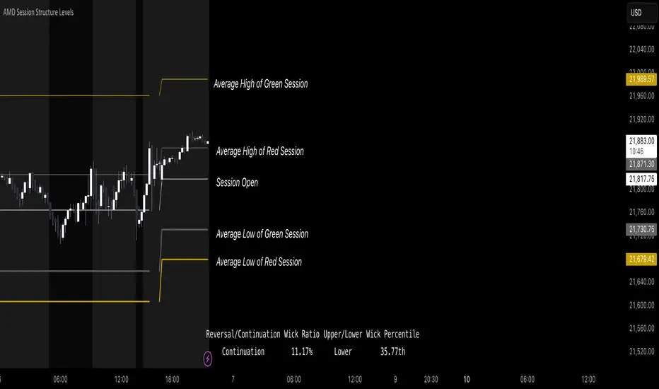
Liquidations Zones [ChartPrime]The Liquidation Zones indicator is designed to detect potential liquidation zones based on common leverage levels such as 10x, 25x, 50x, and 100x. By calculating percentage distances from recent pivot points, the indicator shows where leveraged positions are most likely to get liquidated. It also tracks buy and sell volumes in these zones, helping traders assess market pressure and predict liquidation scenarios. Additionally, the indicator features a heat map mode to highlight areas where orders and stop-losses might be clustered.
⯁ KEY FEATURES AND HOW TO USE
⯌ Leverage Zones Detection :
The indicator identifies zones where positions with leverage ratios of 100x, 50x, 25x, and 10x are at risk of liquidation. These zones are based on percentage moves from recent pivots: a 1% move can liquidate 100x positions, a 4% move affects 25x positions, and so on.
⯌ Liquidated Zones and Volume Tracking :
The indicator displays liquidated zones by plotting gray areas where the price potentually liquidate positons. It calculates the volume needed to liquidate positions in these zones, showing volume from bullish candles if short positions were liquidated and volume from bearish candles for long positions. This feature helps traders assess the risk of liquidation as the price approaches these zones.
⯌ Buy/Sell Volume Calculation :
Buy and sell volumes are calculated from the most recent pivot high or low. For buy volume, only bullish candles are considered, while for sell volume, only bearish candles are summed. This data helps traders gauge the strength of potential liquidation in different zones.
Example of buy and sell volume tracking in active zones:
⯌ Liquidity Heat Map :
In heat map mode, the indicator visualizes potential liquidity areas where orders and stop-losses may be clustered. This map highlights zones that are likely to experience liquidations based on leverage ratios. Additionally, it tracks the highest and lowest price levels for the past 100 bars, while also displaying buy and sell volumes. This feature is useful for predicting market moves driven by liquidation events.
⯁ USER INPUTS
Length : Determines the number of bars used to calculate pivots for liquidation zones.
Extend : Controls how far the liquidation zones are extended on the chart.
Leverage Options : Toggle options to display zones for different leverage levels: 10x, 25x, 50x, and 100x.
Display Heat Map : Enables or disables the liquidity heat map feature.
⯁ CONCLUSION
The Liquidation Zones indicator provides a powerful tool for identifying potential liquidation zones, tracking volume pressure, and visualizing liquidity areas on the chart. With its real-time updates and multiple features, this indicator offers valuable insights for managing risk and anticipating market moves driven by leveraged positions.

Multi-Step FlexiMA - Strategy [presentTrading]It's time to come back! hope I can not to be busy for a while.
█ Introduction and How It Is Different
The FlexiMA Variance Tracker is a unique trading strategy that calculates a series of deviations between the price (or another indicator source) and a variable-length moving average (MA). Unlike traditional strategies that use fixed-length moving averages, the length of the MA in this system varies within a defined range. The length changes dynamically based on a starting factor and an increment factor, creating a more adaptive approach to market conditions.
This strategy integrates Multi-Step Take Profit (TP) levels, allowing for partial exits at predefined price increments. It enables traders to secure profits at different stages of a trend, making it ideal for volatile markets where taking full profits at once might lead to missed opportunities if the trend continues.
BTCUSD 6hr Performance
█ Strategy, How It Works: Detailed Explanation
🔶 FlexiMA Concept
The FlexiMA (Flexible Moving Average) is at the heart of this strategy. Unlike traditional MA-based strategies where the MA length is fixed (e.g., a 50-period SMA), the FlexiMA varies its length with each iteration. This is done using a **starting factor** and an **increment factor**.
The formula for the moving average length at each iteration \(i\) is:
`MA_length_i = indicator_length * (starting_factor + i * increment_factor)`
Where:
- `indicator_length` is the user-defined base length.
- `starting_factor` is the initial multiplier of the base length.
- `increment_factor` increases the multiplier in each iteration.
Each iteration applies a **simple moving average** (SMA) to the chosen **indicator source** (e.g., HLC3) with a different length based on the above formula. The deviation between the current price and the moving average is then calculated as follows:
`deviation_i = price_current - MA_i`
These deviations are normalized using one of the following methods:
- **Max-Min normalization**:
`normalized_i = (deviation_i - min(deviations)) / range(deviations)`
- **Absolute Sum normalization**:
`normalized_i = deviation_i / sum(|deviation_i|)`
The **median** and **standard deviation (stdev)** of the normalized deviations are then calculated as follows:
`median = median(normalized deviations)`
For the standard deviation:
`stdev = sqrt((1/(N-1)) * sum((normalized_i - mean)^2))`
These values are plotted to provide a clear indication of how the price is deviating from its variable-length moving averages.
For more detail:
🔶 Multi-Step Take Profit
This strategy uses a multi-step take profit system, allowing for exits at different stages of a trade based on the percentage of price movement. Three take-profit levels are defined:
- Take Profit Level 1 (TP1): A small, quick profit level (e.g., 2%).
- Take Profit Level 2 (TP2): A medium-level profit target (e.g., 8%).
- Take Profit Level 3 (TP3): A larger, more ambitious target (e.g., 18%).
At each level, a corresponding percentage of the trade is exited:
- TP Percent 1: E.g., 30% of the position.
- TP Percent 2: E.g., 20% of the position.
- TP Percent 3: E.g., 15% of the position.
This approach ensures that profits are locked in progressively, reducing the risk of market reversals wiping out potential gains.
Local
🔶 Trade Entry and Exit Conditions
The entry and exit signals are determined by the interaction between the **SuperTrend Polyfactor Oscillator** and the **median** value of the normalized deviations:
- Long entry: The SuperTrend turns bearish, and the median value of the deviations is positive.
- Short entry: The SuperTrend turns bullish, and the median value is negative.
Similarly, trades are exited when the SuperTrend flips direction.
* The SuperTrend Toolkit is made by @EliCobra
█ Trade Direction
The strategy allows users to specify the desired trade direction:
- Long: Only long positions will be taken.
- Short: Only short positions will be taken.
- Both: Both long and short positions are allowed based on the conditions.
This flexibility allows the strategy to adapt to different market conditions and trading styles, whether you're looking to buy low and sell high, or sell high and buy low.
█ Usage
This strategy can be applied across various asset classes, including stocks, cryptocurrencies, and forex. The primary use case is to take advantage of market volatility by using a flexible moving average and multiple take-profit levels to capture profits incrementally as the market moves in your favor.
How to Use:
1. Configure the Inputs: Start by adjusting the **Indicator Length**, **Starting Factor**, and **Increment Factor** to suit your chosen asset. The defaults work well for most markets, but fine-tuning them can improve performance.
2. Set the Take Profit Levels: Adjust the three **TP levels** and their corresponding **percentages** based on your risk tolerance and the expected volatility of the market.
3. Monitor the Strategy: The SuperTrend and the FlexiMA variance tracker will provide entry and exit signals, automatically managing the positions and taking profits at the pre-set levels.
█ Default Settings
The default settings for the strategy are configured to provide a balanced approach that works across different market conditions:
Indicator Length (10):
This controls the base length for the moving average. A lower length makes the moving average more responsive to price changes, while a higher length smooths out fluctuations, making the strategy less sensitive to short-term price movements.
Starting Factor (1.0):
This determines the initial multiplier applied to the moving average length. A higher starting factor will increase the average length, making it slower to react to price changes.
Increment Factor (1.0):
This increases the moving average length in each iteration. A larger increment factor creates a wider range of moving average lengths, allowing the strategy to track both short-term and long-term trends simultaneously.
Normalization Method ('None'):
Three methods of normalization can be applied to the deviations:
- None: No normalization applied, using raw deviations.
- Max-Min: Normalizes based on the range between the maximum and minimum deviations.
- Absolute Sum: Normalizes based on the total sum of absolute deviations.
Take Profit Levels:
- TP1 (2%): A quick exit to capture small price movements.
- TP2 (8%): A medium-term profit target for stronger trends.
- TP3 (18%): A long-term target for strong price moves.
Take Profit Percentages:
- TP Percent 1 (30%): Exits 30% of the position at TP1.
- TP Percent 2 (20%): Exits 20% of the position at TP2.
- TP Percent 3 (15%): Exits 15% of the position at TP3.
Effect of Variables on Performance:
- Short Indicator Lengths: More responsive to price changes but prone to false signals.
- Higher Starting Factor: Slows down the response, useful for longer-term trend following.
- Higher Increment Factor: Widens the variability in moving average lengths, making the strategy adapt to both short-term and long-term price trends.
- Aggressive Take Profit Levels: Allows for quick profit-taking in volatile markets but may exit positions prematurely in strong trends.
The default configuration offers a moderate balance between short-term responsiveness and long-term trend capturing, suitable for most traders. However, users can adjust these variables to optimize performance based on market conditions and personal preferences.
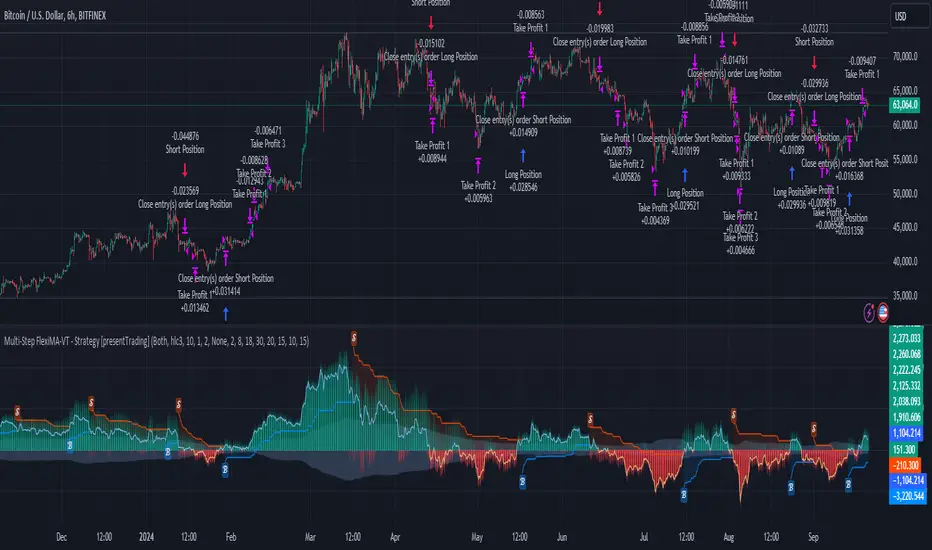
ICT Killzones and Sessions W/ Silver Bullet + MacrosForex and Equity Session Tracker with Killzones, Silver Bullet, and Macro Times
This Pine Script indicator is a comprehensive timekeeping tool designed specifically for ICT traders using any time-based strategy. It helps you visualize and keep track of forex and equity session times, kill zones, macro times, and silver bullet hours.
Features:
Session and Killzone Lines:
Green: London Open (LO)
White: New York (NY)
Orange: Australian (AU)
Purple: Asian (AS)
Includes AM and PM session markers.
Dotted/Striped Lines indicate overlapping kill zones within the session timeline.
Customization Options:
Display sessions and killzones in collapsed or full view.
Hide specific sessions or killzones based on your preferences.
Customize colors, texts, and sizes.
Option to hide drawings older than the current day.
Automatic Updates:
The indicator draws all lines and boxes at the start of a new day.
Automatically adjusts time-based boxes according to the New York timezone.
Killzone Time Windows (for indices):
London KZ: 02:00 - 05:00
New York AM KZ: 07:00 - 10:00
New York PM KZ: 13:30 - 16:00
Silver Bullet Times:
03:00 - 04:00
10:00 - 11:00
14:00 - 15:00
Macro Times:
02:33 - 03:00
04:03 - 04:30
08:50 - 09:10
09:50 - 10:10
10:50 - 11:10
11:50 - 12:50
Latest Update:
January 15:
Added option to automatically change text coloring based on the chart.
Included additional optional macro times per user request:
12:50 - 13:10
13:50 - 14:15
14:50 - 15:10
15:50 - 16:15
Usage:
To maximize your experience, minimize the pane where the script is drawn. This minimizes distractions while keeping the essential time markers visible. The script is designed to help traders by clearly annotating key trading periods without overwhelming their charts.
Originality and Justification:
This indicator uniquely integrates various time-based strategies essential for ICT traders. Unlike other indicators, it consolidates session times, kill zones, macro times, and silver bullet hours into one comprehensive tool. This allows traders to have a clear and organized view of critical trading periods, facilitating better decision-making.
Credits:
This script incorporates open-source elements with significant improvements to enhance functionality and user experience.
Forex and Equity Session Tracker with Killzones, Silver Bullet, and Macro Times
This Pine Script indicator is a comprehensive timekeeping tool designed specifically for ICT traders using any time-based strategy. It helps you visualize and keep track of forex and equity session times, kill zones, macro times, and silver bullet hours.
Features:
Session and Killzone Lines:
Green: London Open (LO)
White: New York (NY)
Orange: Australian (AU)
Purple: Asian (AS)
Includes AM and PM session markers.
Dotted/Striped Lines indicate overlapping kill zones within the session timeline.
Customization Options:
Display sessions and killzones in collapsed or full view.
Hide specific sessions or killzones based on your preferences.
Customize colors, texts, and sizes.
Option to hide drawings older than the current day.
Automatic Updates:
The indicator draws all lines and boxes at the start of a new day.
Automatically adjusts time-based boxes according to the New York timezone.
Killzone Time Windows (for indices):
London KZ: 02:00 - 05:00
New York AM KZ: 07:00 - 10:00
New York PM KZ: 13:30 - 16:00
Silver Bullet Times:
03:00 - 04:00
10:00 - 11:00
14:00 - 15:00
Macro Times:
02:33 - 03:00
04:03 - 04:30
08:50 - 09:10
09:50 - 10:10
10:50 - 11:10
11:50 - 12:50
Latest Update:
January 15:
Added option to automatically change text coloring based on the chart.
Included additional optional macro times per user request:
12:50 - 13:10
13:50 - 14:15
14:50 - 15:10
15:50 - 16:15
ICT Sessions and Kill Zones
What They Are:
ICT Sessions: These are specific times during the trading day when market activity is expected to be higher, such as the London Open, New York Open, and the Asian session.
Kill Zones: These are specific time windows within these sessions where the probability of significant price movements is higher. For example, the New York AM Kill Zone is typically from 8:30 AM to 11:00 AM EST.
How to Use Them:
Identify the Session: Determine which trading session you are in (London, New York, or Asian).
Focus on Kill Zones: Within that session, focus on the kill zones for potential trade setups. For instance, during the New York session, look for setups between 8:30 AM and 11:00 AM EST.
Silver Bullets
What They Are:
Silver Bullets: These are specific, high-probability trade setups that occur within the kill zones. They are designed to be "one shot, one kill" trades, meaning they aim for precise and effective entries and exits.
How to Use Them:
Time-Based Setup: Look for these setups within the designated kill zones. For example, between 10:00 AM and 11:00 AM for the New York AM session .
Chart Analysis: Start with higher time frames like the 15-minute chart and then refine down to 5-minute and 1-minute charts to identify imbalances or specific patterns .
Macros
What They Are:
Macros: These are broader market conditions and trends that influence your trading decisions. They include understanding the overall market direction, seasonal tendencies, and the Commitment of Traders (COT) reports.
How to Use Them:
Understand Market Conditions: Be aware of the macroeconomic factors and market conditions that could affect price movements.
Seasonal Tendencies: Know the seasonal patterns that might influence the market direction.
COT Reports: Use the Commitment of Traders reports to understand the positioning of large traders and commercial hedgers .
Putting It All Together
Preparation: Understand the macro conditions and review the COT reports.
Session and Kill Zone: Identify the trading session and focus on the kill zones.
Silver Bullet Setup: Look for high-probability setups within the kill zones using refined chart analysis.
Execution: Execute the trade with precision, aiming for a "one shot, one kill" outcome.
By following these steps, you can effectively use ICT sessions, kill zones, silver bullets, and macros to enhance your trading strategy.
Usage:
To maximize your experience, shrink the pane where the script is drawn. This minimizes distractions while keeping the essential time markers visible. The script is designed to help traders by clearly annotating key trading periods without overwhelming their charts.
Originality and Justification:
This indicator uniquely integrates various time-based strategies essential for ICT traders. Unlike other indicators, it consolidates session times, kill zones, macro times, and silver bullet hours into one comprehensive tool. This allows traders to have a clear and organized view of critical trading periods, facilitating better decision-making.
Credits:
This script incorporates open-source elements with significant improvements to enhance functionality and user experience. All credit goes to itradesize for the SB + Macro boxes

Heikin Ashi RSI + OTT [Erebor]Relative Strength Index (RSI)
The Relative Strength Index (RSI) is a popular momentum oscillator used in technical analysis to measure the speed and change of price movements. Developed by J. Welles Wilder, the RSI is calculated using the average gains and losses over a specified period, typically 14 days. Here's how it works:
Description and Calculation:
1. Average Gain and Average Loss Calculation:
- Calculate the average gain and average loss over the chosen period (e.g., 14 days).
- The average gain is the sum of gains divided by the period, and the average loss is the sum of losses divided by the period.
2. Relative Strength (RS) Calculation:
- The relative strength is the ratio of average gain to average loss.
The RSI oscillates between 0 and 100. Traditionally, an RSI above 70 indicates overbought conditions, suggesting a potential sell signal, while an RSI below 30 suggests oversold conditions, indicating a potential buy signal.
Pros of RSI:
- Identifying Overbought and Oversold Conditions: RSI helps traders identify potential reversal points in the market due to overbought or oversold conditions.
- Confirmation Tool: RSI can be used in conjunction with other technical indicators or chart patterns to confirm signals, enhancing the reliability of trading decisions.
- Versatility: RSI can be applied to various timeframes, from intraday to long-term charts, making it adaptable to different trading styles.
Cons of RSI:
- Whipsaws: In ranging markets, RSI can generate false signals, leading to whipsaws (rapid price movements followed by a reversal).
- Not Always Accurate: RSI may give false signals, especially in strongly trending markets where overbought or oversold conditions persist for extended periods.
- Subjectivity: Interpretation of RSI levels (e.g., 70 for overbought, 30 for oversold) is somewhat subjective and can vary depending on market conditions and individual preferences.
Checking RSIs in Different Periods:
Traders often use multiple timeframes to analyze RSI for a more comprehensive view:
- Fast RSI (e.g., 8-period): Provides more sensitive signals, suitable for short-term trading and quick decision-making.
- Slow RSI (e.g., 32-period): Offers a smoother representation of price movements, useful for identifying longer-term trends and reducing noise.
By comparing RSI readings across different periods, traders can gain insights into the momentum and strength of price movements over various timeframes, helping them make more informed trading decisions. Additionally, divergence between fast and slow RSI readings may signal potential trend reversals or continuation patterns.
Heikin Ashi Candles
Let's consider a modification to the traditional “Heikin Ashi Candles” where we introduce a new parameter: the period of calculation. The traditional HA candles are derived from the open 01, high 00 low 00, and close 00 prices of the underlying asset.
Now, let's introduce a new parameter, period, which will determine how many periods are considered in the calculation of the HA candles. This period parameter will affect the smoothing and responsiveness of the resulting candles.
In this modification, instead of considering just the current period, we're averaging or aggregating the prices over a specified number of periods . This will result in candles that reflect a longer-term trend or sentiment, depending on the chosen period value.
For example, if period is set to 1, it would essentially be the same as traditional Heikin Ashi candles. However, if period is set to a higher value, say 5, each candle will represent the average price movement over the last 5 periods, providing a smoother representation of the trend but potentially with delayed signals compared to lower period values.
Traders can adjust the period parameter based on their trading style, the timeframe they're analyzing, and the level of smoothing or responsiveness they prefer in their candlestick patterns.
Optimized Trend Tracker
The "Optimized Trend Tracker" is a proprietary trading indicator developed by TradingView user ANIL ÖZEKŞİ. It is designed to identify and track trends in financial markets efficiently. The indicator attempts to smooth out price fluctuations and provide clear signals for trend direction.
The Optimized Trend Tracker uses a combination of moving averages and adaptive filters to detect trends. It aims to reduce lag and noise typically associated with traditional moving averages, thereby providing more timely and accurate signals.
Some of the key features and applications of the OTT include:
• Trend Identification: The indicator helps traders identify the direction of the prevailing trend in a market. It distinguishes between uptrends, downtrends, and sideways consolidations.
• Entry and Exit Signals: The OTT generates buy and sell signals based on crossovers and direction changes of the trend. Traders can use these signals to time their entries and exits in the market.
• Trend Strength: It also provides insights into the strength of the trend by analyzing the slope and momentum of price movements. This information can help traders assess the conviction behind the trend and adjust their trading strategies accordingly.
• Filter Noise: By employing adaptive filters, the indicator aims to filter out market noise and false signals, thereby enhancing the reliability of trend identification.
• Customization: Traders can customize the parameters of the OTT to suit their specific trading preferences and market conditions. This flexibility allows for adaptation to different timeframes and asset classes.
Overall, the OTT can be a valuable tool for traders seeking to capitalize on trending market conditions while minimizing false signals and noise. However, like any trading indicator, it is essential to combine its signals with other forms of analysis and risk management strategies for optimal results. Additionally, traders should thoroughly back-test the indicator and practice using it in a demo environment before applying it to live trading.
The following types of moving average have been included: "SMA", "EMA", "SMMA (RMA)", "WMA", "VWMA", "HMA", "KAMA", "LSMA", "TRAMA", "VAR", "DEMA", "ZLEMA", "TSF", "WWMA". Thanks to the authors.
Thank you for your indicator “Optimized Trend Tracker”. © kivancozbilgic
Thank you for your programming language, indicators and strategies. © TradingView
Kind regards.
© Erebor_GIT

Heikin Ashi TSI and OTT [Erebor]TSI (True Strength Index)
The TSI (True Strength Index) is a momentum-based trading indicator used to identify trend direction, overbought/oversold conditions, and potential trend reversals in financial markets. It was developed by William Blau and first introduced in 1991.
Here's how the TSI indicator is calculated:
• Double Smoothed Momentum (DM): This is calculated by applying double smoothing to the price momentum. First, the single smoothed momentum is calculated by subtracting the smoothed closing price from the current closing price. Then, this single smoothed momentum is smoothed again using an additional smoothing period.
• Absolute Smoothed Momentum (ASM): This is calculated by applying smoothing to the absolute value of the price momentum. Similar to DM, ASM applies a smoothing period to the absolute value of the difference between the current closing price and the smoothed closing price.
• TSI Calculation: The TSI is calculated as the ratio of DM to ASM, multiplied by 100 to express it as a percentage. Mathematically, TSI = (DM / ASM) * 100.
The TSI indicator oscillates around a centerline (typically at zero), with positive values indicating bullish momentum and negative values indicating bearish momentum. Traders often look for crossovers of the TSI above or below the centerline to identify shifts in momentum and potential trend reversals. Additionally, divergences between price and the TSI can signal weakening trends and potential reversal points.
Pros of the TSI indicator:
• Smoothed Momentum: The TSI uses double smoothing techniques, which helps to reduce noise and generate smoother signals compared to other momentum indicators.
• Versatility: The TSI can be applied to various financial instruments and timeframes, making it suitable for both short-term and long-term trading strategies.
• Trend Identification: The TSI is effective in identifying the direction and strength of market trends, helping traders to align their positions with the prevailing market sentiment.
Cons of the TSI indicator:
• Lagging Indicator: Like many momentum indicators, the TSI is a lagging indicator, meaning it may not provide timely signals for entering or exiting trades during rapidly changing market conditions.
• False Signals: Despite its smoothing techniques, the TSI can still produce false signals, especially during periods of low volatility or ranging markets.
• Subjectivity: Interpretation of the TSI signals may vary among traders, leading to subjective analysis and potential inconsistencies in trading decisions.
Overall, the TSI indicator can be a valuable tool for traders when used in conjunction with other technical analysis tools and risk management strategies. It can help traders identify potential trading opportunities and confirm trends, but it's essential to consider its limitations and incorporate additional analysis for more robust trading decisions.
Heikin Ashi Candles
Let's consider a modification to the traditional “Heikin Ashi Candles” where we introduce a new parameter: the period of calculation. The traditional HA candles are derived from the open , high low , and close prices of the underlying asset.
Now, let's introduce a new parameter, period, which will determine how many periods are considered in the calculation of the HA candles. This period parameter will affect the smoothing and responsiveness of the resulting candles.
In this modification, instead of considering just the current period, we're averaging or aggregating the prices over a specified number of periods . This will result in candles that reflect a longer-term trend or sentiment, depending on the chosen period value.
For example, if period is set to 1, it would essentially be the same as traditional Heikin Ashi candles. However, if period is set to a higher value, say 5, each candle will represent the average price movement over the last 5 periods, providing a smoother representation of the trend but potentially with delayed signals compared to lower period values.
Traders can adjust the period parameter based on their trading style, the timeframe they're analyzing, and the level of smoothing or responsiveness they prefer in their candlestick patterns.
Optimized Trend Tracker
The "Optimized Trend Tracker" is a proprietary trading indicator developed by TradingView user ANIL ÖZEKŞİ. It is designed to identify and track trends in financial markets efficiently. The indicator attempts to smooth out price fluctuations and provide clear signals for trend direction.
The Optimized Trend Tracker uses a combination of moving averages and adaptive filters to detect trends. It aims to reduce lag and noise typically associated with traditional moving averages, thereby providing more timely and accurate signals.
Some of the key features and applications of the OTT include:
• Trend Identification: The indicator helps traders identify the direction of the prevailing trend in a market. It distinguishes between uptrends, downtrends, and sideways consolidations.
• Entry and Exit Signals: The OTT generates buy and sell signals based on crossovers and direction changes of the trend. Traders can use these signals to time their entries and exits in the market.
• Trend Strength: It also provides insights into the strength of the trend by analyzing the slope and momentum of price movements. This information can help traders assess the conviction behind the trend and adjust their trading strategies accordingly.
• Filter Noise: By employing adaptive filters, the indicator aims to filter out market noise and false signals, thereby enhancing the reliability of trend identification.
• Customization: Traders can customize the parameters of the OTT to suit their specific trading preferences and market conditions. This flexibility allows for adaptation to different timeframes and asset classes.
Overall, the OTT can be a valuable tool for traders seeking to capitalize on trending market conditions while minimizing false signals and noise. However, like any trading indicator, it is essential to combine its signals with other forms of analysis and risk management strategies for optimal results. Additionally, traders should thoroughly back-test the indicator and practice using it in a demo environment before applying it to live trading.
The following types of moving average have been included: "SMA", "EMA", "SMMA (RMA)", "WMA", "VWMA", "HMA", "KAMA", "LSMA", "TRAMA", "VAR", "DEMA", "ZLEMA", "TSF", "WWMA". Thanks to the authors.
Thank you for your indicator “Optimized Trend Tracker”. © kivancozbilgic
Thank you for your programming language, indicators and strategies. © TradingView
Kind regards.
© Erebor_GIT
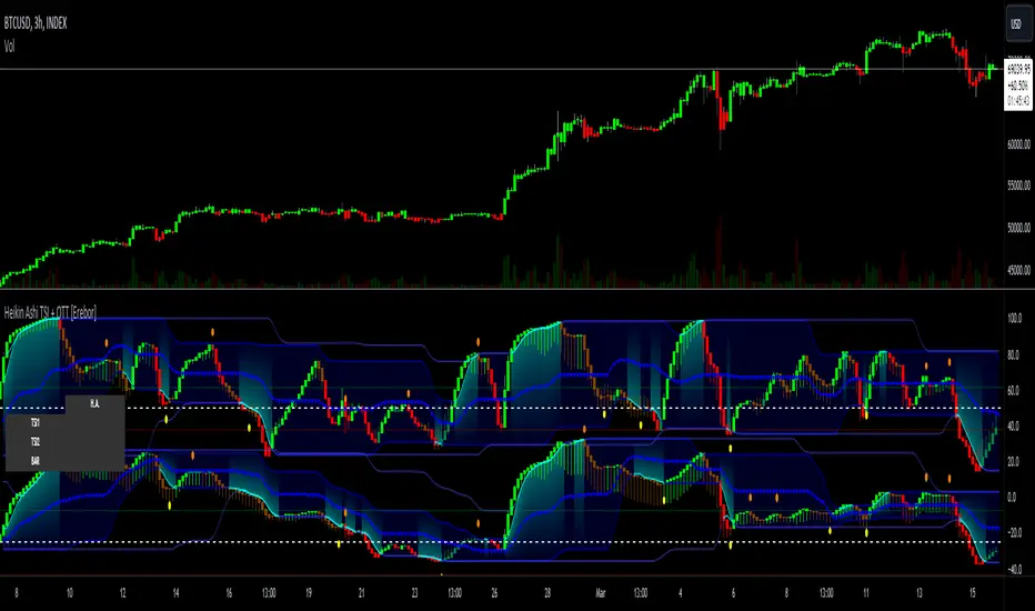
Z Algo (Expo)█ Overview
Z Algo (Expo) is a sophisticated and user-friendly trading tool designed to meet the needs of both novice and seasoned traders. With its real-time signals, trend analysis, and risk management capabilities, this tool can be a valuable addition to any trader's toolkit.
█ Main Features & How to Use
Buy/Sell signals: Z Algo provides real-time buy and sell signals, which assist traders in identifying the most opportune moments to enter or exit a trade.
Strong Buy/Sell signals: In addition to regular buy and sell signals, the tool also offers strong buy and sell signals. These are generated when the market conditions align with a higher probability of a significant price movement.
Sniper Signals: This feature is specifically designed for contrarian traders who look to exploit temporary market inefficiencies or take advantage of price reversals. When enabled, Sniper Signals identify potential market turning points, offering traders the opportunity to profit from sharp price fluctuations.
Reversal Cloud: The Reversal Cloud is a unique visual representation of the market's potential trend reversals. It offers traders an easy-to-understand display of changing market dynamics, enabling them to quickly identify potential entry and exit points based on trend reversals.
Support and Resistance (S/R) Levels: Z Algo automatically calculates and displays support and resistance levels on the chart. These are crucial price points where buying or selling pressure may change, providing valuable insights for traders looking to enter or exit positions based on these levels.
Trend Tracker: This feature helps traders monitor and analyze the prevailing market trend. Trend Tracker identifies and highlights the direction of the trend, allowing traders to align their strategies accordingly and increase their chances of success.
Trend Background Color: To improve the user experience and simplify the interpretation of market data, Z Algo changes the chart's background color based on the identified trend direction. This visual cue makes it easier for traders to recognize bullish or bearish trends at a glance.
Bar Coloring: In addition to the trend background color, Z Algo also provides bar coloring for both contrarian and trend bars. This feature helps traders visualize price movements and trends more effectively, enabling them to identify potential opportunities for both trend-following and contrarian trading strategies.
Risk Management: The tool incorporates risk management features that help traders to protect their capital and maximize potential returns. Users can set stop-loss and take-profit levels, as well as customize their risk exposure according to their individual preferences and trading style.
█ Calculations
█ What are the Buy/Sell signals based on?
The Buy/Sell signals use volatility and price range with a weighting function that can help reduce lag and respond faster to recent price changes. The function gives more weight to the most recent volatility values and absolute price changes, making the algorithm more responsive to changes in volatility and price moves. Using a model that factors in both price changes and volatility gives a bias toward more recent data. This advanced approach to trading signal generation incorporates the concepts of trend following and mean reversion while accounting for changing market volatility.
Traditional systems often use fixed parameters, which may not adapt quickly to changes in market conditions. This can lead to late entries or exits, potentially reducing profitability or increasing risk. Our algorithm uses a weighting function to give more importance to recent volatility values, and absolute price changes can make these signals more responsive. This is especially useful in dynamic markets where price swings and volatility can change rapidly.
Adapting to Recent Price Changes: Markets can often exhibit trending behavior over certain periods. By weighing recent price changes more heavily, the model can quickly identify and react to the emergence of new trends. This can lead to earlier entries in a new trend, potentially increasing profitability.
Adapting to Recent Volatility Changes: Markets can shift from low to high volatility regimes (and vice versa) quite rapidly. A model that gives more weight to recent volatility can adapt its signals to these changing conditions. For example, in high volatility conditions, the model might generate fewer signals to reduce the risk of false breakouts. Conversely, in low volatility conditions, the model might generate more signals to capitalize on trending behavior.
Adaptive Trading: The approach inherently leads to an adaptive trading system. Rather than using fixed parameters, the system can adjust its behavior based on recent market activity. This can lead to a more robust system that performs well across different market conditions.
█ What are the Sniper signals (contrarian signals) based on?
Our contrarian signals are based on deviation from the expected value. The algorithm quantifies the amount of variation or dispersion in a set of values. Non-expected values are the fundamental core of the signal generation process.
█ Reversal Cloud Calculation
The cloud uses the information of how much the price fluctuates over a specific time period and updates its equilibrium value automatically at new price changes. The price changes are used to predict what will happen next, and the band adapts accordingly. The algorithm assumes that past price changes can predict future market behavior.
█ Support and Resistance (S/R) Levels Calculation
The support and resistance levels use historical overbought and oversold levels combined with a weighted atr function to predict future support and resistance areas. This calculation can potentially give traders a great heads-up on where the price may find support and resistance at.
█ Trend & Bar coloring Calculation
Trend calculations with dynamic events are key in ever-changing markets. The main idea of the calculation method is to find the mathematical function that best fits the data points, by minimizing the sum of the squares of the vertical distances of each data point from the equilibrium. The outcome is a function that finds the best mathematical description of that data. Hence the trend output may vary depending on the asset and timeframe. A unique approach where the same settings can give different results.
█ Risk Management Calculation
The risk management system is not unique in itself and contains everything that can help traders to manage their risk, such as different types of stop losses, Take Profits calculations.
-----------------
Disclaimer
The information contained in my Scripts/Indicators/Ideas/Algos/Systems does not constitute financial advice or a solicitation to buy or sell any securities of any type. I will not accept liability for any loss or damage, including without limitation any loss of profit, which may arise directly or indirectly from the use of or reliance on such information.
All investments involve risk, and the past performance of a security, industry, sector, market, financial product, trading strategy, backtest, or individual's trading does not guarantee future results or returns. Investors are fully responsible for any investment decisions they make. Such decisions should be based solely on an evaluation of their financial circumstances, investment objectives, risk tolerance, and liquidity needs.
My Scripts/Indicators/Ideas/Algos/Systems are only for educational purposes!
Script pago

FlashTrade 20 Asset ScreenerThe FlashTrade 20 Asset Screener is a powerful screening tool written in Pinescript and designed for use in Tradingview. It simultaneously monitors a combination of seven (7) lagging and three (3) leading indicators for twenty (20) assets, such as; stocks, cryptocurrencies, or forex pairs.
The screener sends summarized numeric data as an alert to external programs that specialize in automated trading. This proprietary technology developed by the algorithmic trading firm known as FlashTrade.AI is now integrated with the rules-based trading platform TradeLab.AI.
The lagging indicators tracked by the screener are as follows:
1. The 8 Period Exponential Moving Average (8EMA): It determines whether it is over or under the 21 Period Exponential Moving Average (21EMA).
2. Two Closes of the 8 Period Exponential Average (8EMA): This confirms a trend as either bullish or bearish when it occurs over or under the 21 Period Exponential Moving Average (21EMA).
3. Ichimoku Cloud: This indicator identifies whether the price is above or below the cloud, indicating bullish or bearish trends.
4. Ichimoku Cloud: Conversion Line Above Base or Conversion Line Below Base: This measures the trend strength based on the distance between the conversion line and the base line.
5. Ichimoku Cloud: Lag Line Above Price or Lag Line Below Price: This tracks the lag line's position relative to the current price to confirm trend direction.
6. Ichimoku Cloud: Leading Cloud Green or Leading Cloud Red: This identifies the trend based on the color of the leading cloud.
7. MACD: This oscillator tracks the difference between two exponential moving averages and helps identify bullish or bearish momentum in the market.
The screener also tracks three leading indicators that primarily measure trading volume and momentum. These leading indicators are:
1. The Relative Strength Index (RSI): This oscillator measures the speed and change of price movements to identify overbought or oversold conditions in the market.
2. The Stochastic: This oscillator measures the momentum of price movements and helps identify potential trend reversals in the market.
3. The relative Vigor Index (RVGI): This indicator measures the strength of price movements by comparing the closing price to the trading range and helps identify trend reversals.
Overall, the FlashTrade 20 Asset Screener is a powerful tool for traders looking to automate their trading strategies. By monitoring multiple indicators for multiple assets simultaneously, it can identify trends and capitalize on opportunities when they present themselves.

Portfolio_Tracking_TRThis is a portfolio tracker that will track individual, overall and daily profit/loss for up. You can set the size of your buys and price of your buys for accurate, up to date profit and loss data right on your chart. It works on all markets and timeframes.
Next we get into setting up your , order size and price. Each ticker lets you set which stock you bought, then set how much you purchased and then what price you purchased them at.
FEATURES
Top Section
The portfolio tracker has 2 sections. The top section shows each ticker in your portfolio individually with the following data:
- Ticker Name
- Weight of that asset compared to your total portfolio in %
- Current value of that position in TL
- Profit or loss value from purchase price in %
- Todays change in value from yesterday’s close in %
Bottom Section
The bottom section of the tracker will give you info for your portfolio as a whole. It has the following data:
- Total cost of your entire portfolio in TL
- Current value of your entire portfolio in TL
- Current profit or loss of your entire portfolio in TL
- Current profit or loss of your entire portfolio in %
- Todays change of your entire portfolio value compared to yesterday’s close in %
This indicator was compiled from FriendOfTheTrend's indicator named Portfolio Tracker For Stocks & Crypto.

Prophit Ninja: Hidden ScrollStay ahead of the markets moves with "Prophit Ninja: Hidden Scroll".
Our legendary senseis have mastered the arts of wielding the Katana and Shuriken over many decades of focused practice and distilled their systems and techniques down to their most vital form- storing their knowledge in this ancient scroll for easy adoption by any ninja practiced enough to be able to decipher it.
═════════════════════════════════════════════════════════════════════════
█ INTERPRETATION
Each sub-indicator in this package can be used as a confirmation tool to check your bias and give you a more informed decision as they all take into account every reading shown and not shown being calculated across all Prophit Ninja packages. A sentiment rating below the candle shows bullish bias while a green color emphasizes bullish strength- a sentiment rating above the candle shows bearish bias while a red color emphasizes bearish strength- gold color signifies a strong turn in the market while grey/dark grey is a weak reading. A green trend sensei reading is bullish- while a red trend sensei reading is bearish. A green bull trade sensei label signifies a possible bullish trade set up, while a red bear label trade sensei signifies a possible bearish trade set up. Stat sensei gives you tick by tick multi-time frame readings to always keep you aware of the exact environment you're in. Lastly risk sensei will give you the most optimal least risk trade set-up based on user defined variables and give you tick by tick readings of your trade status. This can be used as a standalone decision-maker, or used in confluence with other indicator packages in our Prophit Ninja bundle to get higher precision.
═════════════════════════════════════════════════════════════════════════
█ OVERVIEW
1 — Sentiment Sensei: A toggle-able tick by tick rating system (0-100%) for each candle based on over 100 individual readings .
2 — Trend Sensei: A toggle-able background coloring that easily shows you the trend bias behind the moves.
3 — Trade Sensei: A toggle-able trade finder that finds confluent trade set-ups to give you the upper hand.
4 — Stat Sensei: A toggle-able multi-time frame candle progress tracker with a built in trend bias and price/volume/momentum change/ratio trackers.
5 — Risk Sensei: A toggle-able risk manager with two variations of auto profit target zones , three variations of trailing stop losses , a win/loss tracker , trade duration timer and all the information you need to stay updated with the status of your trade at a glance whether long or short.
═════════════════════════════════════════════════════════════════════════
█ EASY CUSTOMIZATION
i.imgur.com
With a fully customizable and easy-to-use input menu , this indicator gives you the ability to tailor your trading experience to your needs and see as much (or as little) information as you want to; presented in the manner you deem most viable with the following options in just a few clicks:
Indicator Package- This option allows you to switch between the four display modes available so in any moment you can completely change the metrics you’re reading in just two clicks. This allows you the ability to make decisions based on not only what you’re comfortable with; but also to find confirmation or disagreement with other systems instantly.
Color Theme- There are four color themes available which include original, colorful, monochrome and solid. These not only allow you a quick and easy way to change the colors to suit your style; they also make it so you can challenge your bias in an instant by viewing the data in a completely different way.
Dual Attack Modes- Whether you’re a scalper, day trader, swing trader, or investor; this option allows you to see the chart based on four different risk tolerance/time expectancy mentalities for the Katana and Shuriken separately in just two clicks. Investors can see what the scalpers are thinking and vice/versa to broaden their decision making and/or hone in when optimal.
Dual Sharpness Levels- This algorithm allows the user to display the data on five different smoothness levels for the Katana and Shuriken separately without suffering the inherent lag that accompanies most other indicators. Whether you like to see every tick of a choppy movement, or filter out the false signals into smooth readings, you can do so at any moment.
═════════════════════════════════════════════════════════════════════════
█ RISK SENSEI EXAMPLE
═════════════════════════════════════════════════════════════════════════
█ PRE-BUILT ALERTS
With Prophit Ninja: Hidden Scroll's built-in alerts you can enable alerts for any piece of the Hidden Scrollin just a few clicks. These alerts are way more specific and optimized than you can possibly achieve with the custom alert settings. Each checking for multiple possible activation triggers instead of one and populating the message field automatically so you can just click create.
═════════════════════════════════════════════════════════════════════════
As you can see; this ancient scroll has the ability to adapt to any reader or adversary and give those in control of its power the upper hand. Any mode of battle, any opponent, any circumstance- 'Prophit Ninja: Hidden Scroll' was polished by our finest artists to inform any reader and make sure they know when to attack, defend or simply allow the fight to play out by its easy-to-read coloring system. As long as you learn the techniques you'll have a much better chance of making the right decision than when you didn't.
This state-of-the-art tool is great for experienced traders, those who just started learning to trade, or anyone in between- truly made to suit the needs of any trader, in any moment, with any mindset (along with the other indicators in our Prophit Ninja bundle) you'll notice an immediate improvement in your market dexterity after learning it.
═════════════════════════════════════════════════════════════════════════
*everything displayed is part of the Prophit Ninja indicator bundle; this is an otherwise blank chart*

[blackcat] L5 Whale Jump Screener 12 AlertsLinkage Authorization:
When you obtain any one of the following technical indicators authorization, the other one will automatically obtain a free authorization for the same length of time:
1. L5 Whale Jump Screener 25 NoAlerts
2. L5 Whale Jump Screener 12 Alerts
Discount Authorization:
While you are authorized for any of the following technical indicators, this indicator will only need to pay 200TVC (not per month) but you obtain the authorization length as long as your longest one among all invited-only indicators .
1. L5 Whales Jump Out of Ocean X
2. L5 Zen Master
Level: 5
Background:
L5 Whale Jump Screener 12 Alerts is a screeener which is based on principle of L5 Whales Jump Out of Ocean X, but it has its own scheme to work as a screener with alerts, which can track 12 trading pairs at the same time. With this indicator, you can track target in your list with remote alerts from TV to your mobile or emails.
At beginning, I want to incorporate this function to "L5 Whale Jump Screener 25 NoAlerts". However, I found it rather difficult to make it happen. One reason is that adding alerts will further increase computing power of it so that TV will not be functional for overloaded indicators. The only way to make a screen plus alerts happen is to reduce the number of targets allowed in the screener until TV rules are in compliance. The other reason is that I found alerts were conflicting with screener function in TV system during my testing. Because if you put many trading pairs that are highly correlated into inputs of the screener indicator. Huge amount of alerts may be produced at the same time, and TV system has its own protection scheme. If too many alerts happened at the same time, it will block and stop the alert scheme immediately. Therefore, I build this one for anyone who need alert function. But, remember, make input tikerids as NOT correlated as possible to prevent TV to shut down your alert for this indicator.
Function:
By tracking multiple targets with alerts, you will own the capability to tracking multiple markets. This ability will let you know the specific situation of the unconnected market and the trading targets in time in the rotating transaction. The alert function will remind you of the current status of multiple markets via mobile phones and emails.
Inputs:
12 tickerids for your customization
Key Signal:
Long Whales / Banker Pump--> fuchsia color area with 0% transparency
Close Long Whales / Close Banker Pump--> red color area with 0% transparency
Short Whales / Banker Dump --> yellow color area with 0% transparency
Close Short Whales / Close Banker Dump --> green color area with 0% transparency
Long Waves Start--> fuchsia color area with 50% transparency
Short Waves Start --> yellow color area with 50% transparency
No Whale or Wave Signal --> gray color rea with 50% transparency
Pros and Cons:
ONLY suitable for discretionary trading, and does NOT support automatic trading system/bots with alerts.
Intuitive and effective, the output signal is more reliable after multi-indicator resonance
For who does not alert function but track more targets, you can choose anther indicator: L5 Whale Jump Screener 25 NoAlerts.
Why 12 Targets are Supported?
From the principle of TV principle, it should be possible to track up to 40 targets at the same time. However, TV has another condition that restricts server computing resources. When the two condition work at the same time, for the whale jump algorithm, the number of targets it can track at the same time will drop from 40 to about 26~27! In addition, this indicator needs to support the display function from the daily time frame to the 1min time frame. Therefore, the requirements for computing resources have further deteriorated. In the end, the maximum tracking number I obtained by compromise is 25 to ensure that this indicator can support 1min or second level normal display without report an error. Based on above fact, adding alerts will further increase computing power needed for this indicator. To prevent TV shutdown this indicator w/ alerts, only 12 tickerids are supported based on this algorithm. Also, due to quite different user scenarios between these two screeners, two versions are published for different group of traders with a linkage authorization schmeme.
Remarks:
My fourth L5 indicator published
Closed-source
Invite-only
Redeem Fee Life Lock Guarantee
Although I take the efforts to inform the script requesters that the best way to promote trading skills is to learn from the open source scripts I released by themself and to improve their PNIE script programming skills, there are still many people asking how to obtain or pay to use BLACKCAT L4/L5 private scripts. In fact, I do not encourage people to use Tradingview Coins ( TVC ) / Cryptocurrency to redeem the right to use BLACKCAT L4/L5 scripts. However, redeeming private script usage rights through TV Coins/ Cryptocurrency may be an effective way to force more people to learn PINE script programming seriously. And then I can concentrate on answering more valuable community questions instead of being overwhelmed by L4/L5 scripting permission reqeusts.
I would like to announce a ‘Redeem Fee Lock Guarantee’ program to further simplify the L4/L5 indicator/strategy utility offering and distinguish itself from the competition. ‘Redeem Fee lock guarantee’ is one of the major initiatives by BLACKCAT as a part of overall value packaging designed to guard BLACKCAT’s followers’ against cost-overruns and operational risks usually borne by them when it comes to PINE script innovation ecosystem. The TVCs redeemed for L4/L5 a follower signs up for with BLACKCAT is their guaranteed lifetime locked in TVC Quantity/ cryptocurrency, with no special conditions, exclusions and fine print whatsoever. Based on this scheme, I can constantly refine, expand, upgrade and improve PINE script publishing to ensure the very best experiences for my followers. The 'Redeem Fee Lock Guarantee' is a step in the direction of rewarding the valuable followers. NOTE: Every L4/L5 script redeeming service is ONLY limited to TVC or Cryptocurrency ("Win$ & Donate w/ This" Addresses displayed on script page) redeeming which the 1st signed up TVC Qty/ equivalent cryptocurrency is the lifetime offered TVC Qty/ equivalent crypto.
How to subscrible this indicator?
The script subscription period only has two options of one month or one year, and its price is floating. The latest price of the script subscription is proportional to the number of likes/agrees this script has already received. Therefore, the price of subscribing to this script shows an increasing trend, and the earliest subscribers can enjoy the price of lifetime lock to this script. As the number of likes / agrees of this script increases, the subscription fee for one month and one year will also increase linearly. Whatever, the first subscription price of the use will be locked for life.
Monthly subscription and annual subscription can be done either by tradingview coins ( TVC ) or by converting into equivalent cryptocurrency at the exchange rate (1TVC=0.01USD) for redeem.
TVC payment needs to pay TVC directly in the comments under this script. Every time I authorize a new user, I will update the latest number of subscribed users and latest price for next subscription under the script comment. If there are any conflicting scenario happened to the rules and my update. My updated price based on the rule will be the final price for next subscription. The following subscribers need to pay the corresponding amount of TVC or cryptocurrency in accordance with the latest number of users and price announced by me in accordance with the rules published.
TVC redemption is the method I strongly recommend, and I hope you can complete the redemption in the comment area of this script. This is like a blockchain structure, each comment is a block, each subscription is a chain, which is conducive to open and transparent publicity and traceability to avoid unnecessary disputes.
Monthly Subscription Charges
500TVC <50 Agrees (A)
50A<850TVC<100A
100A<1000TVC<150A
150A<1350TVC<200A
200A<1500TVC<250A
250A<1850TVC<300A
300A<2000TVC<350A
350A<2350TVC<400A
400A<2500TVC<450A
450A<2850TVC<500A
500A<3000TVC<550A
550A<3350TVC<600A
600A<3500TVC<650A
650A<3850TVC<700A
700A<4000TVC<750A
750A<4350TVC<800A
800A<4500TVC<850A
850A<4850TVC<900A
900A<5000TVC<950A
950A<5350TVC<1000A
1000A<5500TVC<1050A
And so on...
Annual Subscription Charges
5000TVC <50 Agrees (A)
50A<8500TVC<100A
100A<10000TVC<150A
150A<13500TVC<200A
200A<15000TVC<250A
250A<18500TVC<300A
300A<20000TVC<300A
350A<23500TVC<400A
400A<25000TVC<450A
500A<28500TVC<550A
500A<30000TVC<550A
550A<33500TVC<600A
600A<35000TVC<650A
650A<38500TVC<700A
700A<40000TVC<750A
750A<43500TVC<800A
800A<45000TVC<850A
850A<48500TVC<900A
900A<50000TVC<950A
950A<53500TVC<1000A
1000A<55000TVC<1050A
And so on...

[iQ]PRO Market Structure+ 🚀 PRO Market Structure - Unlocking the Language of the Market
A premium, institutionally-inspired indicator meticulously engineered to decode the complex dynamics of price action and market structure in real-time.
The PRO Market Structure tool provides a clear, objective framework for identifying and tracking the crucial swing points that define market trends. Designed for traders who demand precision, this indicator automatically maps out the high-probability levels of support and resistance, transforming raw price data into actionable structural intelligence.
🧠 Core Intelligence
This advanced tool employs a sophisticated, proprietary logic to pinpoint confirmed market swing highs and swing lows (HH, HL, LH, LL). Unlike simpler methods, our unique state-machine algorithm handles market noise and consolidations with exceptional resilience, ensuring the plotted structure is robust and reliable.
Dynamic Pivot Detection: Utilizes adjustable look-back periods to confirm significant swing points, ensuring you are focused only on structural moves that matter.
Sequential Structure Tracking: The indicator maintains a rigorous internal state, tracking the sequence of structure breaks to distinguish between continuous trend moves and potential reversals.
🔥 Actionable Signal Generation
Move beyond static charting with immediate, intelligent alerts for critical shifts in market control.
BOS (Break of Structure): Automatically detects and marks powerful confirmations of a continuing trend, signaling momentum and directional strength.
CHoCH (Change of Character): Clearly identifies the initial warning signs of a potential trend reversal, highlighting the critical structural level where market balance shifts from bulls to bears, or vice-versa.
Precision and Customization: Signals are generated based on a choice between wick or close penetration, combined with an optional buffer to filter out noise and guarantee high-confidence breaks.
📊 Multi-Timeframe (MTF) Mastery
Gain an unparalleled bird's-eye view of the market with the integrated MTF Structure Panel.
Holistic Context: Simultaneously monitors key market structure on up to three user-defined timeframes, providing essential confluence for high-conviction trade entries.
Advanced Evaluation: The MTF panel offers a proprietary assessment of Trend, Status (BOS/CHoCH), Retracement Percentage, and Key Break Levels for each timeframe, streamlining your top-down analysis into a single, comprehensive view.
✨ Key Features at a Glance
Real-time Level Plotting: Optional plotting of current structural levels (HH, HL, LH, LL) acts as dynamic guides for price action.
Customizable Aesthetics: Full control over colors, line styles, and labeling to integrate seamlessly with your charting setup.
Performance Optimization: Efficient use of Pine Script features, managing object counts to ensure smooth, lag-free operation even on lower timeframes.
The PRO Market Structure is not just an indicator; it is your dedicated structural analyst, providing the objective edge required to navigate complex markets with confidence.

KOBK KILLSHOT PRO V 1.0KOBK KILLSHOT PRO is an advanced trading system that combines multiple layers of technical analysis into one powerful, easy-to-use indicator. Whether you're scalping on lower timeframes or swing trading, this indicator provides crystal-clear entry and exit signals backed by comprehensive market analysis.
## 📝 **TradingView Publication Description**
---
### **Title:**
**KOBK KILLSHOT PRO - Advanced Multi-Timeframe Signal System**
---
### **Short Description:**
Professional-grade trading indicator combining multiple proprietary confirmation layers for high-probability entries and exits. Features intelligent signal quality rating, real-time dashboard, and adaptive exit strategies. Designed for serious traders who demand precision.
---
### **Full Description:**
**KOBK KILLSHOT PRO** is an advanced trading system that combines multiple layers of technical analysis into one powerful, easy-to-use indicator. Whether you're scalping on lower timeframes or swing trading, this indicator provides crystal-clear entry and exit signals backed by comprehensive market analysis.
---
## 🎯 **KEY FEATURES:**
**Smart Signal System:**
- Clear BUY and SELL labels appear directly on your chart
- Quality rating system (★★★★★) shows signal strength
- Early warning dots alert you to potential setups before they trigger
- Color-coded bars show trend direction at a glance
**Real-Time Dashboard:**
- Live ENTRY SIGNAL status (🟢 BUY NOW / 🔴 SELL NOW / ⏳ WAIT)
- Live EXIT SIGNAL status (🟠 EXIT NOW / ✋ HOLD)
- Current position tracking (LONG/SHORT/FLAT)
- Multiple confirmation indicators displayed in real-time
- Trend, momentum, and strength metrics updated every candle
**Flexible Exit Strategies:**
Choose from three exit modes:
- **Flip Mode:** Exit when opposite signal fires (simplest)
- **Momentum Shift:** Exit when momentum changes (faster)
- **Trail Lock:** Trailing stop that locks in profits (let winners run)
**Professional Visuals:**
- Clean, uncluttered chart interface
- Customizable colors and display options
- Toggle individual components on/off
- Works on any timeframe from seconds to daily
---
## 📊 **HOW TO USE IT:**
### **FOR BEGINNERS:**
**Step 1: Add to Chart**
- Apply KOBK KILLSHOT PRO to your chart
- Default settings work great for most traders
- Recommended timeframes: 15-second to 15-minute for active trading
**Step 2: Watch for Signals**
- **GREEN "BUY" label** = Enter LONG position
- **RED "SELL" label** = Enter SHORT position
- **Orange "EXIT" X** = Close your position
- Check the dashboard in top-right corner for confirmation
**Step 3: Follow the Quality Rating**
- **★★★★★ (5 stars)** = Highest probability setup - take these!
- **★★★★☆ (4 stars)** = Strong setup - good to trade
- **★★★☆☆ (3 stars)** = Decent setup - use caution
- **Lower ratings** = Skip unless very experienced
**Step 4: Use the Dashboard**
The live HUD tells you everything you need:
- **Entry Signal:** Shows when to enter (BUY NOW / SELL NOW / WAIT)
- **Exit Signal:** Shows when to exit (EXIT NOW / HOLD)
- **Position:** Tracks if you're LONG, SHORT, or FLAT
- **Quality:** Current signal strength rating
---
### **FOR ADVANCED TRADERS:**
**Customization Options:**
- Adjust signal sensitivity via Key Value parameter
- Control ATR period for different market conditions
- Enable/disable individual filter components
- Choose signal quality threshold (Maximum/High/Medium/Standard)
- Select preferred exit strategy based on trading style
**Filter System:**
The indicator includes multiple proprietary filters that can be toggled individually:
- Trend alignment filters
- Momentum confirmation filters
- Volatility filters
- Flow strength analysis
- Key zone detection
**Signal Quality Control:**
Set minimum quality requirements:
- **Maximum:** Only 5-star signals (very selective)
- **High:** 4-star minimum (recommended for most)
- **Medium:** 3-star minimum (more opportunities)
- **Standard:** 2-star minimum (active trading)
- **All Signals:** Every signal (experienced only)
---
## ⚙️ **RECOMMENDED SETTINGS:**
**For Scalping (15-second to 1-minute charts):**
- Key Value: 1.0
- ATR Period: 10
- Signal Quality: High (4-star minimum)
- Exit Mode: Flip or Momentum Shift
**For Day Trading (5-minute to 15-minute charts):**
- Key Value: 1.0 to 1.5
- ATR Period: 14
- Signal Quality: High
- Exit Mode: Trail Lock
**For Swing Trading (1-hour+ charts):**
- Key Value: 1.5 to 2.0
- ATR Period: 14-20
- Signal Quality: Maximum (5-star only)
- Exit Mode: Trail Lock
---
## 🎮 **SIMPLE TRADING RULES:**
1. **Wait for the signal** - Don't predict, let the indicator tell you
2. **Check the stars** - Higher quality = higher probability
3. **Verify the dashboard** - Make sure Entry Signal shows BUY NOW or SELL NOW
4. **Enter immediately** - When signal fires, don't hesitate
5. **Follow the exit** - When EXIT NOW appears, close the position
6. **Be disciplined** - Trust the system, don't override it
---
## ⚠️ **IMPORTANT NOTES:**
- **Not a holy grail:** No indicator is perfect. Use proper risk management.
- **Backtest first:** Test on demo/paper account before using real money.
- **Position sizing matters:** Never risk more than 1-2% per trade.
- **Market conditions vary:** Some days are better than others.
- **Combine with fundamentals:** Technical signals work best with good market context.
---
## 🔧 **DISPLAY OPTIONS:**
Toggle on/off as needed:
- Live Dashboard (HUD)
- Signal Quality Stars
- Early Warning Signals
- Key Zone Markers
- Trend Lines
- Additional confirmation indicators
---
## 📈 **BEST MARKETS TO USE:**
Works on any liquid market:
- Futures (NQ, ES, YM, etc.)
- Forex pairs (major and minor)
- Crypto (BTC, ETH, etc.)
- Stocks (high volume)
- Indices
---
## 💡 **PRO TIPS:**
1. **Start with higher quality settings** (4-5 stars only) until you're comfortable
2. **Use the early warning dots** to prepare for entries (get your finger ready)
3. **Pay attention to the dashboard trend indicator** - trade with the trend
4. **Don't trade during major news events** - wait for clear market direction
5. **Keep a trading journal** - track which star ratings work best for your style
6. **Adjust Key Value if needed** - higher = fewer signals, lower = more signals
---
## 🎯 **WHAT MAKES THIS DIFFERENT:**
Unlike simple indicators that just draw lines or show one metric, KOBK KILLSHOT PRO combines multiple proprietary analysis layers into one cohesive system. The intelligent filtering ensures you only see high-probability setups, while the real-time dashboard keeps you informed of market conditions every step of the way.
The star rating system is particularly powerful - it instantly tells you how many confirmation factors are aligned, so you can make quick decisions about which signals to take and which to skip.
---
## 📞 **SUPPORT:**
For questions, setup help, or optimization tips, feel free to reach out via TradingView messages. I'm here to help you succeed with this system!
---
**Disclaimer:** This indicator is for educational and informational purposes only. Trading involves substantial risk. Past performance does not guarantee future results. Always use proper risk management and never trade with money you can't afford to lose.
---
## 🏆 **START TRADING SMARTER TODAY**

FVG DUAL HTF ALERTS FINAL DG FVG Dual HTF - Advanced Fair Value Gap Detector with Confluence & Strength Analysis
Professional-grade Fair Value Gap (FVG) detection system designed for precision trading on Gold and other instruments.
🎯 Key Features
Dual Higher Timeframe Analysis
HTF1 & HTF2 Detection: Simultaneously monitors two higher timeframes (default: 15min & 60min) for Fair Value Gaps
Multi-timeframe Confluence: Automatically detects when FVGs align across multiple timeframes for high-probability setups
Customizable Timeframes: Choose from 5min, 15min, 60min, 4H, or Daily for each HTF
Intelligent Strength Scoring System (0-11 Scale)
Our proprietary algorithm rates each FVG based on:
Gap size relative to ATR
Volume analysis vs. average
Current timeframe confluence (★ symbol indicates FVG exists on your chart timeframe)
Session timing (London & New York priority)
HTF confluence bonus
Color-Coded Ratings:
🟢 Lime (8-11): Premium strength - highest probability setups
🟡 Yellow (5-7): Good strength - solid opportunities
⚪ Gray (0-4): Weak strength - proceed with caution
Sweet Spot Entry Zones
Inner Box Technology: Highlights the optimal 10% entry zone within each FVG
BUY/SELL Labels: Clear visual cues for directional bias
Automatic Entry/Stop/Target Lines: Shows precise risk-reward setups on the 3 nearest FVGs
Position Sizing Calculator: Displays dollar values based on your lot size
Advanced Fill Methods
Choose how FVGs are invalidated:
Wick Sweep: Most conservative - requires price to sweep through the gap
Any Touch: Price touches the FVG boundary
Midpoint Reached: 50% fill required
Body Beyond: Strictest - candle body must close through the gap
Comprehensive Market Intelligence Table
Real-time monitoring of:
Gold Daily & Hourly Bias (with pip movement)
BTC Daily & Hourly Bias (optional)
Distance to nearest Bull/Bear FVGs
IN ZONE Indicator: 🔥 Alerts when price enters premium sweet spots
Shows strength rating and HTF source
Color-coded: Premium / Good / Weak / Out
Professional Alert System
HTF1 & HTF2 Zone Entry Alerts
Sweet Spot Entry Alerts (BUY/SELL)
High-Strength FVG Alerts (8+ rating)
Combined "ANY HTF" alerts for maximum flexibility
📊 Default Configuration
Optimized for Gold (XAU/USD) on 3-minute charts
Session Focus: London (8am-12pm GMT) & New York (1:30pm-4pm GMT)
Risk Management: Built-in R:R calculator with customizable stops and targets
🎨 Customization Options
Multiple color schemes for bull/bear zones
Adjustable inner box percentage
Confluence highlighting (bright colors when HTF1 & HTF2 align)
Show/hide individual components
BTC correlation tracking (optional)
⚙️ Technical Specifications
Maximum Display: Up to 50 FVGs per type (HTF1 Bull/Bear, HTF2 Bull/Bear)
Fill Tracking: Monitors touched vs. untouched zones
Lookback Period: Configurable (default: 100 bars for current TF confluence)
Body Close Requirement: Optional strict mode for cleaner signals
📈 Best Used For
Gold (XAU/USD) day trading
Institutional order flow analysis
High-probability reversal setups
Multi-timeframe confirmation strategies
Risk-reward optimization
🔒 Access & Support
This is a private indicator. Contact the owner for details about access and usage.
Disclaimer: This indicator is a tool for technical analysis. Past performance does not guarantee future results. Always use proper risk management and trade responsibly.
Short Version (if space is limited):
FVG Dual HTF - Professional Fair Value Gap System
Advanced FVG detector with dual higher timeframe analysis, intelligent strength scoring (0-11), and multi-timeframe confluence detection. Features sweet spot entry zones, automatic R:R lines, real-time IN ZONE alerts, and comprehensive market intelligence table.
Highlights:
🎯 Dual HTF monitoring (15m/60m default)
⭐ Strength scoring with current TF confluence (★)
📊 Color-coded ratings: Lime (8+) / Yellow (5-7) / Gray (<5)
🎨 Sweet spot inner boxes with BUY/SELL signals
🔔 Professional alert system
💰 Built-in position sizing calculator
📈 Gold Daily/Hourly + BTC bias tracking
Optimized for Gold and BTC. Multiple fill methods, customizable colors, and extensive settings.
Contact owner for access details.
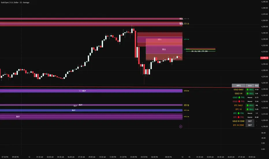
LHAMA MTF Structure & Fibs [LTS]Overview
LHAMA MTF Structure & Fibs is a multi-purpose market structure toolkit that combines current-timeframe structure, higher-timeframe structure, Imbalance/FVG-based order blocks, and automatic Fibonacci retracements into a single chart overlay.
Current-Timeframe Structure
The indicator first maps current-timeframe market structure using swing highs and lows based on a user-defined pivot length (“Time-Horizon”):
Labels swing points as HH , HL , LH , and LL .
Draws BOS (Break of Structure) when price breaks beyond a prior swing.
Optionally identifies CHoCH (Change of Character) when a break occurs against the previous direction.
Lets you choose whether BOS/CHoCH confirmation uses closes or wicks .
Provides options to show/hide swing labels, choose line style (solid/dashed/dotted), and configure bullish/bearish colors.
Higher-Timeframe (HTF) Structure
On top of the local structure, the script builds a higher-timeframe structure map and projects it onto your active chart:
Aggregates price into HTF “bars” (e.g., 4h structure on a 5m chart).
Detects HTF pivots with their own pivot length setting.
Draws HTF BOS/CHoCH lines and labels back on the lower timeframe.
Lets you choose wick vs close confirmation for HTF breaks.
Optional “ pending ” HTF levels: lines extended from the latest HTF swing highs/lows that remain “waiting” until price breaks them.
This is designed to make it easier to see how intraday price is moving relative to the dominant higher-timeframe trend.
Order Blocks (Imbalance/FVG-Based)
The indicator detects simple bullish and bearish order blocks based on fair value gaps and prior sweeps:
Identifies bullish/bearish FVGs together with a sweep of a previous low/high.
Creates colored boxes anchored to an “anchor” candle and extends them forward.
Marks boxes as “broken” when price trades inside or through the opposite side.
Broken blocks can have reduced emphasis (more transparent, dashed border) and can optionally be deleted.
Show Nearest Only mode highlights only the closest active bullish and bearish blocks to reduce chart clutter.
Periodic cleanup removes very old boxes to maintain chart responsiveness.
Automatic Fibonacci Levels
The script can draw up to five customizable Fibonacci retracement levels using the HTF structure logic:
Measures swings using HTF pivots and extremes.
Historical mode : measures between two confirmed pivots in one direction.
Live mode : starts from the last confirmed pivot and tracks the evolving extreme; if price reverses through that pivot, measurement can flip to track the new leg.
Each Fib level has its own on/off toggle, ratio value, and color.
Draws a main swing line plus retracement lines projected slightly into the future.
Key Inputs & Customization
Market Structure (Current TF)
Pivot length (“Time-Horizon”).
BOS confirmation: candle close or wicks.
BOS/CHoCH line style and width.
Swing labels on/off and global label size.
Bullish/bearish colors.
Market Structure (HTF)
HTF timeframe selection.
Separate pivot length for HTF swings.
Close vs wick confirmation for HTF breaks.
HTF swing labels and CHoCH labels on/off.
Pending HTF levels: style, color, and visibility.
Order Block Settings
Bullish/bearish box colors and border width.
Maximum number of boxes to display.
Optional deletion of broken blocks.
“Show Nearest Only” filter to highlight the closest active zones.
Max bars to backscan for the anchor candle.
Cleanup frequency for removing very old boxes.
Fibonacci Settings
Show/hide auto Fibs.
Historical vs Live tracking mode.
Five user-defined ratios with individual toggles and colors.
