Dynamic Momentum OscillatorDescription:
The Dynamic Momentum Oscillator is a statistically-driven momentum tool that goes beyond traditional oscillators. Instead of using raw price, it analyzes the momentum of a DEMA (Double Exponential Moving Average) itself, creating a smoother, more refined signal. Its innovative approach incorporates volatility-weighted z-scoring, allowing the indicator to automatically adjust its sensitivity based on market conditions, helping to identify both the strength and sustainability of momentum shifts.
🔍 How It Works:
DEMA Momentum Core: The indicator first calculates a DEMA of the price. It then analyzes the momentum of this DEMA, effectively creating a "momentum of momentum" measure that filters out market noise.
Volatility-Adaptive Z-Score: The core signal is a statistical z-score, which measures how many standard deviations the DEMA is from its mean. This tells you not just the direction, but the statistical significance of the move.
Dynamic Volatility Weighting: The unique addition is a normalized standard deviation component that weights the z-score. In high volatility periods, this amplifies the signal, making strong trends more pronounced. In low volatility, it provides a more muted, conservative output.
🎯 Interpreting the Oscillator:
Zero Line: The baseline. Momentum is considered neutral here.
Orange Histogram (Above Zero): Indicates bullish momentum. The further the bar extends above zero, the stronger and more statistically significant the bullish momentum.
Purple Histogram (Below Zero): Indicates bearish momentum. The further the bar extends below zero, the stronger and more statistically significant the bearish momentum.
Signal Strength: The height of the histogram bars reflects the combined momentum and volatility, giving you a direct visual gauge of momentum strength.
⚙️ Input Parameters (Group: Core Settings):
DEMA Length: The period for the primary Double Exponential Moving Average.
Standard Deviation Length: The lookback period for calculating volatility and the z-score.
StDev Weight: Controls the influence of volatility on the final signal (0.1 = minimal, 1.0 = maximum). Adjust this to fine-tune the indicator's responsiveness.
By focusing on the statistical properties of price momentum, the Dynamic Momentum Oscillator offers a unique lens for pinpointing high-probability trend continuations and reversals. It's a powerful tool for traders who appreciate quantitative methods.
M-oscillator

Alpha-Weighted RSIDescription:
The Alpha-Weighted RSI is a next-generation momentum oscillator that redefines the classic RSI by incorporating the mathematical principles of Lévy Flight. This advanced adaptation applies non-linear weighting to price changes, making the indicator more sensitive to significant market moves and less reactive to minor noise. It is designed for traders seeking a clearer, more powerful view of momentum and potential reversal zones.
🔍 Key Features & Innovations:
Lévy Flight Alpha Weighting: At the core of this indicator is the Alpha parameter (1.0-2.0), which controls the sensitivity to price changes.
Lower Alpha (e.g., 1.2): Makes the indicator highly responsive to recent price movements, ideal for capturing early trend shifts.
Higher Alpha (e.g., 1.8): Creates a smoother, more conservative output that filters out noise, focusing on stronger momentum.
Customizable Smoothing: The raw Lévy-RSI is smoothed by a user-selectable moving average (8 MA types supported: SMA, EMA, SMMA, etc.), allowing for further customization of responsiveness.
Intuitive Centered Oscillator: The RSI is centered around a zero line, providing a clean visual separation between bullish and bearish territory.
Dynamic Gradient Zones: Subtle, colour coded gradient fills in the overbought (>+25) and oversold (<-25) regions enhance visual clarity without cluttering the chart.
Modern Histogram Display: Momentum is plotted as a sleek histogram that changes color between bright cyan (bullish) and magenta (bearish) based on its position relative to the zero line.
🎯 How to Use & Interpret:
Zero-Line Crossovers: The most basic signals. A crossover above the zero line indicates building bullish momentum, while a crossover below suggests growing bearish momentum.
Overbought/Oversold Levels: Use the +25/-25 and +35/-35 levels as dynamic zones. A reading above +25 suggests strong bullish momentum (overbought), while a reading below -25 indicates strong bearish momentum (oversold).
Divergence Detection: Look for divergences between the Alpha-Weighted RSI and price action. For example, if price makes a new low but the RSI forms a higher low, it can signal a potential bullish reversal.
Alpha Tuning: Adjust the Alpha parameter to match market volatility. In choppy markets, increase alpha to reduce noise. In trending markets, decrease alpha to become more responsive.
⚙️ Input Parameters:
RSI Settings: Standard RSI inputs for Length and Calculation Source.
Lévy Flight Settings: The crucial Alpha factor for response control.
MA Settings: MA Type and MA Length for smoothing the final output.
By applying Lévy Flight dynamics, this indicator offers a nuanced perspective on momentum, helping you stay ahead of the curve. Feedback is always welcome!

CG Momentum - Table🇹🇭 คำอธิบาย (ภาษาไทย)
CG Momentum - Table
อินดิเคเตอร์นี้ถูกออกแบบมาเพื่อใช้ตรวจสอบสภาพตลาดและโมเมนตัมในหลาย Timeframe พร้อมกันในรูปแบบ “ตาราง” ที่เข้าใจง่าย ช่วยให้ผู้ใช้งานสามารถประเมินแรงซื้อ/แรงขาย และแนวโน้มของตลาดในภาพรวมได้อย่างรวดเร็ว โดยไม่ต้องเปิดหลายหน้าจอหรือสลับกราฟบ่อย ๆ
✅ องค์ประกอบหลักที่แสดงในตาราง
คอลัมน์ ความหมาย
TF ช่วงเวลา (Timeframe) ที่ใช้วิเคราะห์
W%R ระบุโซน Overbought / Oversold ของราคา (ค่าในช่วง 0..-100)
Stoch %K วัดแรงดีดตัวและความเร็วของการเคลื่อนที่ของราคาในช่วงสั้น
MACD ± วัดทิศทางโมเมนตัมด้วยการดูความชันของ MACD (ขึ้นต่อเนื่อง = + , ลงต่อเนื่อง = -)
RSI ± วัดพลังของราคาโดยเปรียบเทียบ RSI กับค่าเฉลี่ยของตัวมันเอง (RSI > SMA(RSI) = + , RSI < SMA(RSI) = -)
🎯 จุดประสงค์ของอินดิเคเตอร์นี้
เพื่อช่วยประเมิน สภาวะตลาดในหลาย TF อย่างรวดเร็ว
ใช้เป็น เครื่องมือยืนยันสัญญาณร่วม กับระบบเทรดเดิม
มองเห็นจุดที่ตลาด เริ่มเปลี่ยนแรง / เปลี่ยนโมเมนตัม
ลดการเข้าออเดอร์ผิดฝั่งในช่วงที่ตลาดอ่อนแรงหรือแกว่งตัว
🧠 แนวคิดการนำไปใช้งาน
มองหาช่วงที่ หลาย TF ให้สัญญาณไปในทิศทางเดียวกัน
ตัวอย่างโซนเข้า Long ที่น่าสนใจ:
W%R อยู่ใกล้ Oversold
Stoch เริ่มดีดขึ้น
MACD เป็น +
RSI เป็น +
การที่สัญญาณหลายตัว “ตรงกัน” เท่ากับมี ความน่าจะเป็นสูงขึ้น
⚠️ หมายเหตุสำคัญ
อินดิเคเตอร์นี้เป็น เครื่องมือช่วยตัดสินใจ ไม่ใช่สัญญาณเข้าออกเพียงอย่างเดียว
ควรใช้ร่วมกับ:
แนวรับ / แนวต้าน
โครงสร้างราคา (Structure)
Volume หรือ Price Action
===============================================================
===============================================================
🇺🇸 English Description
W%R & Stoch + MACD + RSI Multi-Timeframe Momentum Dashboard
This indicator provides a clean and efficient momentum overview across multiple timeframes.
It displays key oscillator and momentum signals in a structured table, making it easy to assess whether the market is trending, reversing, or ranging without switching charts.
✅ Table Columns Explained
Column Meaning
TF Timeframe being analyzed
W%R Identifies Overbought / Oversold price conditions (0..-100 scale)
Stoch %K Measures short-term price momentum and bounce strength
MACD ± Momentum slope direction (MACD rising for 2 bars = “+”, falling = “-”)
RSI ± RSI strength relative to its SMA (RSI > RSI SMA = “+”, RSI < RSI SMA = “-”)
🎯 Purpose of This Indicator
To provide multi-timeframe momentum context at a glance
To act as a confirmation tool alongside your existing strategy
To help identify momentum shifts and trend continuation signals
To reduce false entries in weak or choppy market conditions
🧠 How to Use
Look for alignment across multiple timeframes:
Example for bullish setup:
W%R near Oversold
Stoch turning upward
MACD shows “+”
RSI shows “+”
The more alignment → the stronger the probability of a successful entry.
⚠️ Disclaimer
This indicator is a decision support tool, not a standalone entry signal.
Use together with:
Support / Resistance zones
Market Structure
Volume or Price Action confirmation

Valdex BBWP MultitimeframeValdex BBWP Multitimeframe: Multitimeframe Volatility at Your Fingertips
Created by:
Adaptation of: Bollinger Band Width Percentile (BBWP)
// --- GENERAL DESCRIPTION ---
The **Valdex BBWP Multitimeframe** indicator is an advanced and optimized adaptation of the classic *Bollinger Band Width Percentile (BBWP)* indicator. Its purpose is to provide a robust and flexible tool for measuring the market's **relative volatility** on a scale from 0 to 100.
What distinguishes this version is its ability to **analyze volatility across THREE timeframes simultaneously**, allowing you to confirm expansion (high volatility) or contraction (low volatility) in higher timeframes without switching charts. It is an essential filter for any breakout or retracement strategy.
// --- KEY FEATURES ---
1. Base Line (Current TF): Displays the BBWP calculated on the exact timeframe of the current chart, preserving its pure, unsmoothed value (original "noise").
2. Multitimeframe (MTF) Lines: Allows you to define two separate BBWP lines, each pulling data from an external timeframe (e.g., 60 minutes, Daily). Includes a configurable Moving Average (MA) to smooth the noise.
3. Key References: Includes horizontal lines at 0, 50, and 100 for quick zone identification.
// --- CONFIGURATION AND USAGE ---
For MTF Lines 2 and 3, you must manually enter the desired timeframe in the text field (valid examples: 5, 60, 240, D, W).
----------------------------------------------------------------------
🇪🇸 Versión en Español: Valdex BBWP Multitimeframe: La Volatilidad Multitemporal
El indicador Valdex BBWP Multitimeframe es una adaptación optimizada del BBWP. Mide la volatilidad relativa del mercado en una escala del 0 al 100, simultáneamente en TRES temporalidades distintas. Es un filtro esencial para cualquier estrategia basada en rupturas o retrocesos.
Funcionalidades Clave:
1. Línea Base (TF Actual): Coincide con el BBWP puro de la temporalidad del gráfico actual (sin suavizar).
2. Líneas Multitemporales (MTF): Permite definir dos líneas de BBWP separadas, extrayendo datos de una temporalidad externa (ej.: 60 minutos, Diario). Incluye una Media Móvil (MA) configurable para suavizar el ruido.

Valdex BBWP Multitimeframe🇬🇧 (English Version)
Valdex BBWP Multitimeframe: Multitimeframe Volatility.
**Created by:**
**Adaptation of: Bollinger Band Width Percentile (BBWP)
📄 General Description
The **Valdex BBWP Multitimeframe** indicator is an advanced and optimized adaptation of the classic *Bollinger Band Width Percentile (BBWP)* indicator. Its purpose is to provide a robust and flexible tool for measuring the market's **relative volatility** on a scale from 0 to 100.
What distinguishes this version is its ability to **analyze volatility across THREE timeframes simultaneously**, allowing you to confirm expansion (high volatility) or contraction (low volatility) in higher timeframes without switching charts. It is an essential filter for any breakout or retracement strategy.
✨ Key Features
The indicator plots three volatility lines, each with a specific and independently configurable purpose:
1. **Base Line (Current TF):** Displays the BBWP calculated on the **exact timeframe of the current chart**, preserving its pure, unsmoothed value (original "noise").
2. **Multitimeframe (MTF) Lines:** Allows you to define two completely separate BBWP lines, each pulling data from an **external timeframe** (e.g., 60 minutes, Daily). Includes a **configurable Moving Average (MA)** to smooth the noise.
⚙️ Configuration and Usage
* **BBWP Base Settings:** You can configure the underlying BBWP parameters: Bands Length (13 default) and Percentile Lookback (252 default).
* **MTF Configuration:** For Lines 2 and 3, you **must manually enter** the desired timeframe in the text field (valid examples: `5`, `60`, `240`, `D`, `W`).

OsMA by A8/4 - Limited Edition🌟 **OsMA by A8/4 — The Ultimate Indicator for XAUUSD Trading** 🌟
An intelligent **automated system** designed exclusively for **gold trading**, equipped with everything you need in one tool 🔥
💡 **Key Features of OsMA by A8/4**
✅ **Auto Entry Signals**
Automatically detects trade opportunities using a **refined MACD Histogram formula** for enhanced accuracy.
Displays **LONG/SHORT arrows only on the first bar** to keep your chart clean and readable.
✅ **Auto Take Profit & Stop Loss System (Auto TP/SL)**
Once a signal appears, the system automatically sets:
* **TP1 = +15 USD**
* **TP2 = +25 USD**
* **SL = -10 USD**
These levels are displayed as **dashed lines** on the chart — clear and updated in real-time.
✅ **Smart DCA System (3 Orders)**
Works for both LONG and SHORT positions:
* **Order 1:** Entry upon signal confirmation (after candle close)
* **Order 2:** Entry at 5 USD below/above Order 1
* **Order 3:** Entry at another 5 USD below/above Order 2
The system automatically **calculates the average entry price** and **adjusts the SL** to -10 USD from the average cost.
This helps **spread risk** and **increase recovery potential** when prices rebound 💰
✅ **Specially Designed for XAUUSD Trading**
Compatible with both **Spot Gold** and **TFEX Gold Futures**.
Perfect for traders who value **clear, structured entry and exit strategies**.

Stochastic Triple Momentum by SidHemA precision-tuned Stochastic system combining MTF (Multi Time Frame) momentum, Divergence detection, and market pressure scoring.
Full Description:
Stochastic Triple Momentum by SidHem is a performance-focused oscillator designed for traders who want deeper momentum insight without chart clutter. It enhances the classic Stochastic with three high-value features:
The "Triple Momentum" refers to:
Stochastic slope momentum
RSI momentum zone
MFI money flow bias
1) Multi-Timeframe Stochastic
Compare local swings against higher timeframe momentum.
Turn it on when you want trend confirmation across intraday → swing → positional context.
2) Full Divergence Engine (Regular + Hidden)
Automatically detects:
Regular Bullish / Regular Bearish Divergence
Hidden Bullish / Hidden Bearish Divergence
Visual style options:
Labels on the stochastic panel
Swing-to-swing Divergence Lines
Each divergence category has independent color, width, and label size controls.
3) Trend Strength Meter + Heat Strip
Momentum pressure is scored using:
Stochastic slope direction
RSI position relative to 50
MFI (Money Flow Index) position relative to 50
This produces a clear bias/sentiment reading:
Strong Bear → Bearish → Weak Bear → Neutral → Weak Bull → Bullish → Strong Bull
Displayed as:
A Trend Strength Label (movable to multiple panel positions)
A Heat Strip at the bottom of the panel for quick visual bias
Additional Customization:
Adjustable %K / %D smoothing
Selectable line style, width, opacity
Overbought / Oversold bands with independent styling
Classic / Modern / Heatmap background shading modes
Optional RSI and MFI overlays
Panel locked to 0-100 for consistent scaling
Ideal Usage:
Use higher timeframes (e.g., 4H / Daily) for trend bias.
Use divergences + %K/%D crossovers for precise entry timing.
Use Trend Meter and Heat Strip to filter out weak signals.
This indicator works on:
Stocks
Index Futures
Crypto
Forex
Commodities
Any timeframe

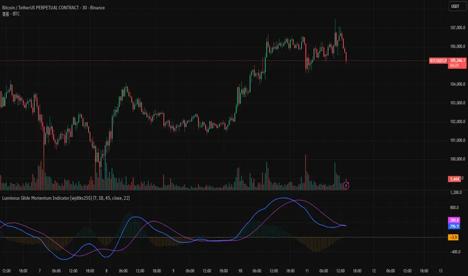
Luminous Glide Momentum Indicator [wjdtks255]This indicator, named "Customized SuperSmoother MA Oscillator," applies a smoothing filter to price data using a SuperSmoother technique to reduce noise and enhance signal clarity. It calculates two moving averages on the smoothed data—a fast and a slow—whose difference forms the oscillator line. A signal line is derived by smoothing the oscillator with another moving average. The histogram visualizes the divergence between the oscillator and signal lines, indicating momentum strength and direction.
How it works
SuperSmoother Filter: Reduces price noise to provide smoother and more reliable signals than raw data.
Fast and Slow Moving Averages: The fast MA reacts quicker to price changes, while the slow MA indicates longer trends.
Oscillator: The difference between the fast and slow MAs signals shifts in momentum.
Signal Line: A smoothed version of the oscillator used to generate crossovers.
Histogram: Displays the distance between the oscillator and signal line, with color changes indicating bullish or bearish momentum.
Trading Strategy
Buy Signal: When the oscillator crosses above the signal line, it suggests increasing upward momentum, signaling a potential buy opportunity.
Sell Signal: When the oscillator crosses below the signal line, it suggests increasing downward momentum, signaling a potential sell opportunity.
Histogram Size and Color: Larger green bars indicate stronger bullish momentum; larger red bars indicate stronger bearish momentum.
Usage Tips
Combine this oscillator with other indicators or price action analysis to confirm trading signals.
Adjust smoothing and moving average lengths according to your trading timeframe and the asset volatility.
Use proper risk management to filter out potential false signals common in oscillators.
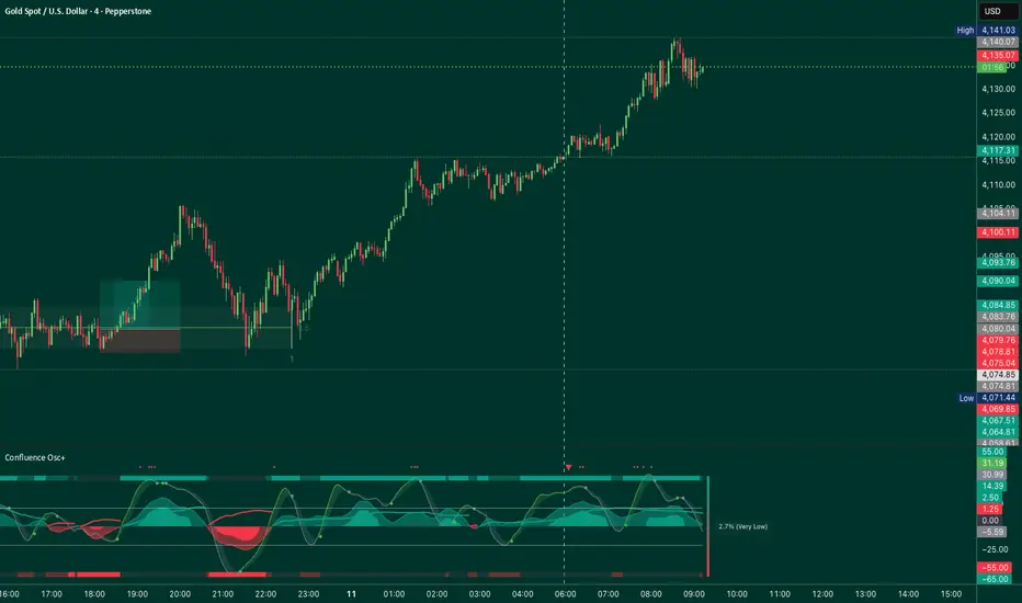
Confluence Oscillator EnhancedThe **Confluence Oscillator** (Enhanced by Sila) is a sophisticated multi-component trading indicator that combines four powerful analytical tools to provide comprehensive market analysis. This indicator integrates oscillator signals, money flow analysis, confluence detection, and reversal identification to help traders make informed decisions.
1. **Hyper Wave Oscillator
- Primary momentum oscillator with signal smoothing
- Divergence detection capabilities
- Crossover/crossunder signal generation
2. Smart Money Flow (MFI)
- Modified Money Flow Index analysis
- Volume-weighted price momentum
- Bullish/bearish flow tracking
3. Confluence System
- Real-time confluence percentage calculation
- Visual confluence meter and areas
- Multi-component signal alignment
4. Reversal Detection
- Volume-based reversal signals
- Major and minor reversal identification
- RSI-enhanced volume analysis
5. Delta Footprint (coming soon)
Z-Score of RSI//@version=5
indicator("Z-Score of RSI", overlay=false)
// Tham số
rsi_length = input.int(14, "RSI Length")
z_length = input.int(60, "Z-Score Period")
// Tính RSI
rsi = ta.rsi(close, rsi_length)
// Tính Z-Score
mean_rsi = ta.sma(rsi, z_length)
std_rsi = ta.stdev(rsi, z_length)
z_rsi = (rsi - mean_rsi) / std_rsi
// Vẽ biểu đồ
plot(z_rsi, color=color.new(color.aqua, 0), linewidth=2, title="Z-Score(RSI)")
hline(0, "Mean", color=color.gray)
hline(2, "Overbought (+2σ)", color=color.red)
hline(-2, "Oversold (-2σ)", color=color.lime)
// Cảnh báo (tuỳ chọn)
bgcolor(z_rsi < -2 ? color.new(color.lime, 85) : na)
bgcolor(z_rsi > 2 ? color.new(color.red, 85) : na)

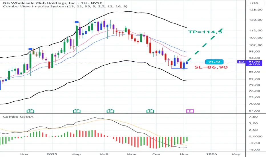
Combo OsMAMACD + OsMA Combo shows classic MACD (12,26,9) lines together with a colored OsMA histogram. Histogram bars change color based on momentum: one color for increasing bars, another for decreasing. Helps visualize trend strength and momentum shifts.
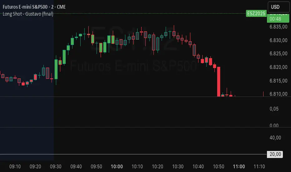
Long Shot ESPurpose: Highlights trend direction and strength to support quick trading decisions.
Advantages: Candle coloring, visual arrows for key signals, status table for indicators, and configurable alerts for real-time notifications.
How to Use: Follow colored candles and arrows to identify trend opportunities, check the status table for confirmation, and use alerts to act on important signals.
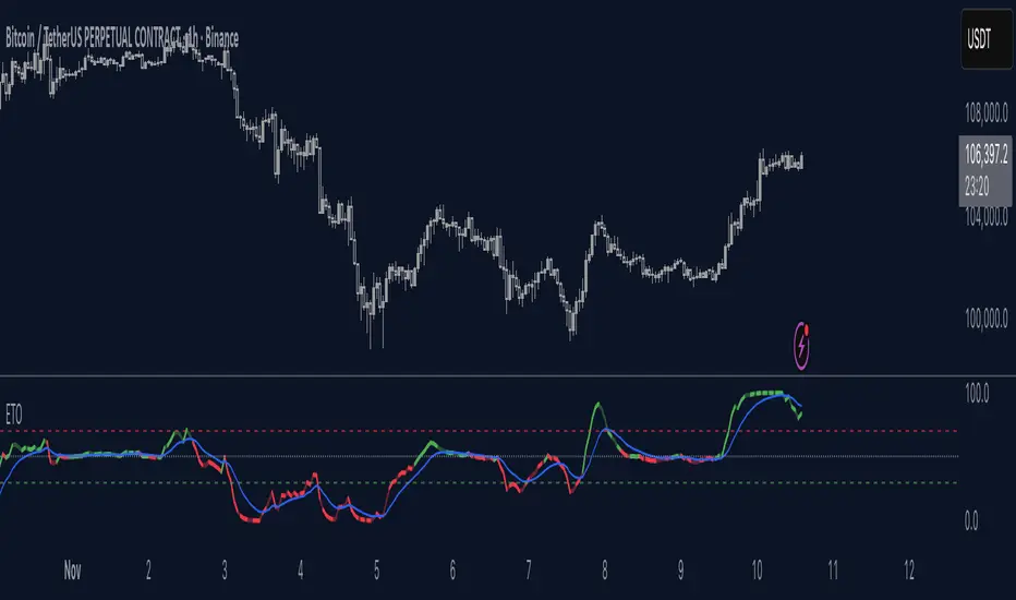
Elastic Trend OscillatorThe Elastic Trend Oscillator (ETO) is a volatility-adaptive momentum indicator that measures price displacement from a trend baseline while accounting for market volatility conditions. Unlike traditional oscillators that use fixed scaling, ETO dynamically adjusts its sensitivity based on current volatility levels relative to recent market conditions, providing context-aware momentum readings across different market regimes.
What Makes This Indicator Different
Volatility-Adaptive Scaling:
The core innovation of ETO is its dynamic volatility adjustment mechanism. The indicator calculates an ATR percentile rank over a lookback period and uses this to scale the momentum readings. When volatility is elevated, the indicator becomes less sensitive to price moves, recognizing that larger displacements are normal in volatile conditions. Conversely, in low volatility environments, smaller price moves are given more weight. This prevents false signals during volatility expansions and maintains sensitivity during quiet periods.
Low Volatility Compression:
During periods of extremely low volatility, the oscillator naturally compresses toward the midline and exhibits minimal movement. This midline-hugging behavior serves as a visual indicator that the market lacks directional energy and momentum readings are unreliable. Unlike indicators that continue oscillating during quiet periods and potentially generate false signals, ETO's compression around the midline is supposed to identify low-conviction environments where trend-following strategies underperform. When you see the oscillator stuck near 50 with little movement, recognize this as a consolidation phase where ranges dominate and breakout setups may be developing.
Trend Slope Analysis with Dynamic Thresholds:
The indicator monitors both the trend direction (EMA slope) and the rate of slope change. Dynamic thresholds based on ATR identify when trend acceleration is slowing. The oscillator becomes semi-transparent when slope deceleration exceeds the threshold, warning of potential trend exhaustion before actual reversals occur.
Relatively Linear Transformation:
Unlike many oscillators that use non-linear transformations, ETO applies a more linear scaling of the ATR-normalized displacement. This preserves the proportional relationship between price moves and oscillator readings, making divergences and momentum shifts more intuitive to interpret.
How to Use the Indicator
Trend Direction:
Green oscillator = Bullish trend (price above EMA with positive slope)
Red oscillator = Bearish trend (price below EMA with negative slope)
Oscillator compressed near 50 with minimal movement = Low volatility, consolidation phase. These phases often precede volatility expansions and significant directional moves, making them more ideal for monitoring breakout setups rather than taking positions.
Momentum Quality:
Solid color = Strong, accelerating trend
Semi-transparent = Decelerating trend, potential exhaustion, potential consolidation ahead
The transparency change acts as an early warning before actual trend reversals or consolidations.
Trading Signals:
Crossovers: When the oscillator crosses the signal line to the other side of momentum while oversold/overbought, it suggests potential reversals (better in combination with transparency loss).
Overbought/Oversold: Levels above 70 indicate overbought conditions; below 30 indicate oversold. These are not reversal signals themselves but identify extended moves where momentum may be extreme.
Midline: Oscillator above 50 indicates price is above the trend baseline with positive displacement. Below 50 indicates negative displacement.
Divergences: Like with other momentum indicators compare oscillator highs/lows with price highs/lows.
Settings
EMA Length: Controls the trend baseline period. Lower values make the indicator more responsive to short-term price changes; higher values focus on longer-term trends. This directly affects how quickly the oscillator responds to trend changes.
ATR Length: Determines the period for volatility measurement. This affects both the normalization of price displacement and the momentum confirmation filter. Lower values make volatility measurements more reactive; higher values provide smoother volatility assessment.
Oscillator Smoothing: Applies EMA smoothing to the raw oscillator values. A value of 1 shows unsmoothed, more volatile readings. Higher values produce smoother oscillations with less noise but more lag.
Signal Line Length: The EMA period for the signal line. Lower values create more frequent crossovers; higher values generate fewer but potentially more significant crossovers. This acts as a moving average of the oscillator itself.
Slope Change Sensitivity: Multiplier that sets how much slope deceleration triggers the transparency effect. Lower values make the indicator more sensitive to trend exhaustion, showing transparency earlier. Higher values require more pronounced deceleration before visual warning.
Overbought Level: Defines the upper extreme threshold.
Oversold Level: Defines the lower extreme threshold.
Best Practices
Use on any timeframe, but adjust EMA and ATR lengths according to your trading style (shorter for shorter term trades, longer for longer term trading like swing trading)
Combine with price action — the indicator identifies momentum conditions, not specific entry/exit points.
In strongly trending markets, the oscillator may remain in overbought/oversold territory for extended periods—this is normal and indicates persistent momentum rather than imminent reversal.
This indicator does not provide investment or trading advice. All trading decisions should be made based on your own analysis and risk management.
ADX FAST and NOICE FREE DIThis tool is designed to identify trend strength and direction earlier than the traditional ADX/DI system.
Instead of relying on the normal Wilder smoothing, this version applies momentum projection to ADX (Fast ADX)
and then filters all directional movement signals through Hull smoothing to minimize market noise.
The result:
• Trends are detected faster
• Pullbacks are filtered more cleanly
• Sideways or weak structures become easy to avoid
Recommended Usage:
• Look for Fast ADX above the threshold to confirm trend environment
• Use Noise-Free +DI and -DI to confirm trend direction (bullish / bearish dominance)
• Background color highlights only when trend + direction are aligned
This is not a buy/sell signal generator by itself; it is best used as a trend and market condition confirmation layer.
Disclaimer:
This script is provided for educational and informational purposes only.
It does not constitute financial advice or a recommendation to buy or sell any security.
Market conditions vary and past performance does not guarantee future results.
Always perform your own analysis and risk management, and trade responsibly.

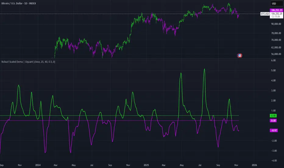
Robust Scaled Dema | OquantOverview
The Robust Scaled DEMA indicator is a tool designed for traders seeking to identify potential trend directions in financial markets. It combines the smoothing capabilities of a Double Exponential Moving Average (DEMA) with a robust scaling mechanism to normalize the data, making it more resilient to outliers and extreme price movements. This scaling helps in generating long and short signals based on predefined thresholds, visualized through color-coded plots and bars. The indicator aims to provide a balanced view of market momentum, reducing the impact of noise while highlighting significant shifts in price behavior.
Key Factors/Components
DEMA (Double Exponential Moving Average): Serves as the core smoothing component, reducing lag compared to simple averages by emphasizing recent price action more effectively.
Robust Scaling Mechanism: Utilizes statistical measures like median and interquartile range to normalize the DEMA values, ensuring the indicator is less sensitive to extreme values or price spikes.
Thresholds: User-defined upper and lower levels that trigger long or short signals when the scaled DEMA crosses them.
Visual Elements: Includes plotted lines for the scaled DEMA and thresholds, plus color-coded candlestick bars for intuitive interpretation.
Alerts: Built-in conditions for notifying users of potential entry points for long or short positions.
How It Works
The indicator starts by applying a DEMA to the chosen price source to create a smoothed representation of the market's direction. This smoothed value is then scaled using a robust statistical approach that accounts for the distribution of recent DEMA values, centering it around a median and adjusting for variability to minimize the influence of outliers. The resulting scaled metric is compared against user-set upper and lower thresholds: crossing above the upper suggests a bullish momentum (long signal), while dipping below the lower indicates bearish conditions (short signal). A state variable tracks these conditions to color the chart accordingly, helping traders visualize regime changes. Optional alerts fire on transitions.
For Who Is Best/Recommended Use Cases
This indicator is ideal for traders who employ trend-following or momentum-based strategies and need tools that perform well in non-normal market conditions, such as during high volatility or in assets prone to spikes. Use cases include identifying entry/exit points in trending environments, confirming breakouts, or integrating into multi-indicator systems for added confirmation. Quantitative traders or those backtesting strategies will appreciate its customizable parameters for optimization.
Settings and Default Settings
Source: The price data input for calculations, such as close, open, high, or low. Default: close.
DEMA Length: Controls the period for the DEMA smoothing; shorter values increase responsiveness but may add noise, longer ones provide more lag but smoother signals. Default: 25.
Robust Scaling Length: Defines the lookback period for the scaling statistics; affects how adaptive the normalization is to recent data distributions. Default: 40.
Upper Threshold: The level above which a long signal is triggered; higher values make signals rarer but potentially more reliable. Default: 0.5.
Lower Threshold: The level below which a short signal is triggered; lower values allow for more aggressive bearish detection. Default: 0.
Conclusion
The Robust Scaled DEMA offers an outlier-resistant alternative to traditional moving average indicators, empowering traders to navigate volatile markets. By blending exponential smoothing with statistical robustness, it provides actionable insights into trend shifts while minimizing false positives from extreme events..
⚠️ Disclaimer: This indicator is intended for educational and informational purposes only. Trading/investing involves risk, and past performance does not guarantee future results. Always test and evaluate indicators/strategies before applying them in live markets. Use at your own risk.
HTF MACD Dual Zero Cross + First EMA PullbackThis script aims to get the trader on the right side of the momentum and get better entries by only alerting when price pulls back to the trader's specified EMA.
This script isnt meant to catch tops or bottoms but to trade with the momentum once it starts.
This script will alert whe nthe MACD and signal line both cross the zero line, after that the script waits for price to make a pullback and then alet either a sell or buy. Ive found this works best when you trade with the trend on a higher timeframe.
You can use whatever MACD settings you prefer and really customize this to the asset youre trading.
You can also change whether you get an alert based on a wick touch of the EMA or a candle close.

Supertrend Dual-Zone Channel V2**Supertrend Dual-Zone Channel V2**
Advanced Supertrend with Dual-Zone Visualization, Breakout Counter, and Dynamic Labels
A powerful upgrade to the classic Supertrend indicator that displays two distinct zones:
• Bullish Channel (green): Active when price is above the Supertrend line
• Bearish Channel (red): Active when price is below the Supertrend line
Key Features
• Dual-Zone Fill System: Clearly separates bullish and bearish regimes with semi-transparent channel fills for instant trend context.
• Reverse Tracking Lines: Shows the opposite-direction Supertrend band (faint green/red lines) to highlight potential reversal zones.
• Automatic Breakout Counter: Counts consecutive breaks into the opposite tracking band.
- Green labels below bars: Bullish breakouts (price closes above bearish tracking line while in uptrend)
- Red labels above bars: Bearish breakouts (price closes below bullish tracking line while in downtrend)
• Clean Label Management: Uses arrays to store labels with tooltips showing breakout sequence number.
• Mid-Channel Reference: Invisible midline based on (high + low)/2 for internal fill logic (not plotted).
How to Use
• Strong Trend Confirmation: Price staying within its colored channel = healthy trend.
• Pullback Entries: Look for price touching the faint reverse tracking line without breaking it.
• Breakout Signals: Labeled breakouts (1st, 2nd, 3rd...) often precede trend exhaustion or acceleration.
• Works on all timeframes and assets.
Inputs
• Factor (default: 3.0) – Sensitivity of the Supertrend bands
• ATR Period (default: 10) – Lookback period for volatility calculation
Visuals
• Thick green/red line: Current active Supertrend
• Faint opposite-color line: Reverse tracking band
• Light green/red fills: Bullish/Bearish zones
• Numbered labels: Sequential breakout counter
Fully optimized with max_lines_count=500 and max_labels_count=500.
Clean, lightweight, and highly readable on chart.
Version 2 – Improved labeling, better zone separation, and smarter counter reset on trend change.
Perfect for trend-following, pullback trading, and spotting potential reversals.
Happy trading!
====================================================================================
**Supertrend 双区通道 V2**
高级超级趋势指标:双色通道可视化 + 突破计数器 + 动态标签
经典 Supertrend 的强力升级版,通过 **双区通道** 直观区分多空状态:
• 多头通道(绿色):价格位于 Supertrend 上方时激活
• 空头通道(红色):价格位于 Supertrend 下方时激活
### 核心功能
• 双区填充系统:半透明通道填色,一眼分辨当前多空主导区域
• 反向轨道线:显示对立方向的 Supertrend 带(淡绿/淡红虚线),清晰标记潜在反转区域
• 自动突破计数器:统计价格连续突破反向轨道的行为
- 绿色标签(K线下方):多头突破(多头趋势中收盘突破空头轨道)
- 红色标签(K线上方):空头突破(空头趋势中收盘跌破多头轨道)
• 智能标签管理:使用数组存储标签,带工具提示显示突破序号
• 通道中轴:基于 (high + low)/2 的隐形中线,仅用于填充逻辑(不显示)
### 使用方法
• 趋势健康:价格始终停留在同色通道内 = 强势趋势
• 回调入场:价格触及淡色反向轨道但未突破 = 优质回调机会
• 突破信号:连续编号突破(第1次、第2次…),根据不同品种设定自定义的突破次数,btc通常五次突破后才会衰竭。
• 适用于所有周期、所有品种
### 输入参数
• 倍数(默认 3.0):控制 Supertrend 带的灵敏度
• ATR周期(默认 10):波动率计算周期
### 视觉元素
• 粗实线(绿/红):当前生效的 Supertrend 主线
• 细虚线(淡绿/淡红):反向轨道线
• 浅色填充:多头/空头通道区域
• 编号标签:突破序号(从0开始计数)
**V2 版升级**:优化标签逻辑、更好区域分隔、趋势切换时自动归零计数器。
祝交易顺利!

Atilla Triple Confirm PRO v7 — MACD + RSI + STC + Volume Power Atilla Triple Confirm PRO v7 is an advanced trend and momentum analysis system that uses a triple technical confirmation + volume filter.
Components:
MACD: Identifies trend reversals and momentum direction.
RSI: Measures overbought/oversold zones and momentum.
STC (Schaff Trend Cycle): Indicates price momentum and trend maturity.
VolFeatures:
"LONG READY / SHORT READY / STOP" alert system
Confirmation Strength (%): Dynamically calculates how many indicators are in the same direction
Divergence Detector: Displays price differences with the RSI
Center-right panel: Small, simple, and mobile-friendly info box
Automatic Alert Support: Sends notifications when LONG / SHORT are ready
Heikin Ashi & Regular Candlestick Compatible
⚙️ Usage Recommendation:
When "LONG READY" occurs, it is recommended that the price be supported by trend confirmation from the 50 EMA or STC.
When "SHORT READY" occurs, an RSI crossing below 50 is considered a strong signal.
Trading confidence is high when Confirmation Strength is 75% or above.
🧭 Fully compatible with Atilla STC Dynamic TP Systems.ume Filter: Confirms breakouts supported by increased volume.

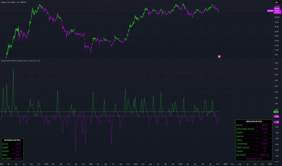
Robust Scaled HMA | OquantOverview
The Robust Scaled HMA indicator is a trend-following tool, leveraging a Hull Moving Average (HMA) with robust statistical scaling to generate buy and sell signals. It helps traders identify potential entry and exit points for long and short positions while providing comprehensive performance metrics to evaluate the strategy's effectiveness compared to a simple buy-and-hold approach(remember past performance doesn’t guarantee future results). By incorporating outlier-resistant scaling, it aims to deliver smoother, more adaptive signals in volatile markets. The indicator also visualizes allocation signals, equity curves, and key metrics in intuitive tables, empowering users to make data-driven decisions without relying on overly complex optimizations.
Key Factors/Components
Hull Moving Average (HMA): A fast and smooth moving average that reduces lag compared to traditional averages, serving as the core trend detector.
Robust Scaling Mechanism: Uses statistical measures like median and interquartile range (IQR) to normalize the HMA, making it resistant to extreme price outliers and potentially improving signal reliability in noisy markets.
Threshold-Based Signals: Customizable upper and lower thresholds to trigger long (bullish) or short (bearish) allocations, with options to enable/disable longs or shorts for strategy customization.
Performance Metrics Suite: Calculates performance metrics including Maximum Drawdown (Max DD), Intra-Trade Max DD, Sharpe Ratio, Sortino Ratio, Omega Ratio, Percent Profitable Trades, Profit Factor, Total Trades, and Net Profit.
Equity Curve and Visualization: Optional plotting of the strategy's equity curve, along with color-coded bars and candles for visual signal confirmation.
Comparative Analysis: Includes a buy-and-hold metrics table for benchmarking the indicator's performance against passive holding(remember past performance doesn’t guarantee future results).
Alert Conditions: Built-in alerts for bullish and bearish signals to notify users of potential trade opportunities.
How It Works
The indicator starts by applying a HMA to the selected price source to capture the underlying trend with minimal lag. This average is then scaled using robust statistical methods that focus on the central tendency and spread of recent data, filtering out the impact of extreme price swings for a more stable output. Signals are generated when the scaled value crosses predefined thresholds: exceeding the upper threshold indicates a potential long position (bullish momentum), while dropping below the lower threshold suggests a short position (bearish momentum). The system simulates a simple strategy by allocating to long, short, or cash based on user preferences, tracking returns over time from a specified start date. It then computes a range of performance metrics by analyzing the equity curve, drawdowns, and trade outcomes, presenting them alongside buy-and-hold equivalents for easy comparison(remember past performance doesn’t guarantee future results). This logic promotes trend-following while emphasizing risk management, without overcomplicating the process.
For Who Is Best/Recommended Use Cases
This indicator is best suited for traders focused on trend-following strategies in markets prone to volatility or outliers. Recommended use cases include: Trend Identification: As a filter for entering/exiting positions. Strategy Evaluation: Quickly assessing signal quality through integrated metrics without complex backtesting setups(Remember past performance doesn’t guarantee future results). Customization: Adjusting for bullish biases by disabling shorts, or vice versa, in one-sided markets.
Settings and Default Settings
The indicator offers flexible inputs grouped for ease of use:
Start Date: Defines the backtesting period (default: January 1, 2018) to ensure metrics are calculated from a relevant historical point.
Source: The price data input for calculations (default: close price).
HMA Length: Period for the Hull Moving Average (default: 25) – shorter values increase sensitivity, longer ones smooth out noise.
Robust Scaling Length: Window for statistical scaling (default: 40)
Upper Threshold: Level for triggering long signals (default: 0.6) – higher values make signals more conservative.
Lower Threshold: Level for triggering short signals (default: -0.2) – lower (more negative) values require stronger bearish confirmation.
Allow Long Trades: Enables long positions (default: true); if false, longs default to cash.
Allow Short Trades: Enables short positions (default: false); if false, shorts default to cash.
Show Indicator Metrics Table: Displays indicator performance table (default: true).
Show Buy&Hold Table: Displays benchmark metrics table (default: true).
Plot Equity Curve: Visualizes the strategy's cumulative returns (default: false).
Conclusion
The Robust Scaled HMA offers a fresh take on trend detection by prioritizing robustness through IQR scaling, making it a valuable addition for traders aiming to navigate noisy markets with metrics-backed insights(Remember past performance doesn’t guarantee future results).
⚠️ Disclaimer: This indicator is intended for educational and informational purposes only. Trading/investing involves risk, and past performance does not guarantee future results. Always test and evaluate indicators/strategies before applying them in live markets. Use at your own risk.
oppliger trendfollow📈 Strategy Overview: SMA25 vs SMA200 – Gap Momentum Trend Strategy
This strategy is a trend-following system designed to capture strong, accelerating uptrends while exiting early when momentum begins to fade.
It uses the relationship between two moving averages — the 25-period SMA and the 200-period SMA — and monitors the gap (distance) between them as a measure of trend strength.
🟢 Entry Conditions (Go Long)
A long position is opened only when all of the following conditions are true:
Uptrend confirmation:
The 25-period SMA is above the 200-period SMA
→ confirms a clear upward trend.
Price momentum:
The closing price is above the SMA25 line,
→ showing that the market currently trades with bullish momentum.
Trend acceleration:
The gap between SMA25 and SMA200 has been increasing for the last 5 consecutive bars.
→ mathematically:
gap_t > gap_(t-1) > gap_(t-2) > gap_(t-3) > gap_(t-4)
→ indicates that the short-term trend is pulling away from the long-term trend and accelerating upward.
✅ When all three conditions are met, the strategy enters a long trade at the close of the current candle.
🔴 Exit Conditions (Close Long)
The position is closed when the uptrend starts to lose strength:
Trend deceleration:
The gap between SMA25 and SMA200 has been shrinking for 3 consecutive bars.
→ mathematically:
gap_t < gap_(t-1) < gap_(t-2)
→ signals that the short-term moving average is converging toward the long-term average, showing weakening momentum.
🚪 When this condition is met, the strategy closes the position at market price.
⚙️ Summary of Logic
Phase Condition Meaning
Entry SMA25 > SMA200 Long-term trend is up
Entry Close > SMA25 Short-term momentum is bullish
Entry Gap rising 5 bars Trend is accelerating
Exit Gap falling 3 bars Trend is weakening
💡 Interpretation
This strategy aims to:
Enter only when a strong, accelerating uptrend is confirmed.
Stay in the trade as long as momentum remains intact.
Exit early when the market starts losing strength, before the trend fully reverses.
It works best in trending markets and helps avoid false entries during sideways or weak phases.

Twiggs Go Money Flow Enhanced [KingThies]█ OVERVIEW
The Twiggs Money Flow (TMF) is a volume-weighted momentum oscillator that
measures buying and sellistng pressure by analyzing where price closes within
each bar's true range. It's an enhanced version of Chaikin Money Flow that
uses Wilder's smoothing method, providing better trend persistence and
smoother signals.
The indicator oscillates around a zero listne:
Values above zero indicate accumulation (buying pressure)
Values below zero indicate distribution (sellistng pressure)
TMF was developed by Colistn Twiggs as an improvement over traditional money
flow indicators by incorporating true range calculations and Wilder's
exponential moving average.
█ CONCEPTS
True Range Boundaries
TMF calculates a modified true range for each bar by comparing the current
bar's high and low with the previous close:
True Range High = maximum of (previous close, current high)
True Range Low = minimum of (previous close, current low)
This accounts for overnight gaps and ensures price continuity between bars.
Average Daily Value (ADV)
The ADV represents the portion of volume attributable to buying versus sellistng:
ADV = Volume × ((Close - TR Low) - (TR High - Close)) / True Range
When price closes near the high of the true range, ADV is positive and large.
When price closes near the low, ADV is negative and large.
A close in the middle produces values near zero.
Wilder's Moving Average
Unlistke simple moving averages, Wilder's smoothing method gives more weight
to recent values while maintaining memory of historical data:
WMA = (Previous WMA × (Period - 1) + Current Value) / Period
This creates smoother trends that are less prone to whipsaws than standard
moving averages.
Final Calculation
TMF = Wilder's MA(ADV, Period) / Wilder's MA(Volume, Period)
By dividing smoothed ADV by smoothed volume, TMF normalistzes the reading and
makes it comparable across different securities and timeframes.
█ HOW TO USE
Zero listne Crossovers
The most straightforward trading signals:
A cross above zero suggests buyers are gaining control.
Consider this a bullistsh signal, especially when confirmed by price action.
A cross below zero suggests sellers are gaining control.
Consider this a bearish signal.
The longer TMF remains above or below zero, the stronger the trend.
Extreme Values
Strong positive or negative readings indicate intense buying or sellistng pressure:
Sustained high positive values (above +0.4) suggest strong accumulation
but may also indicate overbought conditions.
Sustained low negative values (below -0.4) suggest strong distribution
but may also indicate oversold conditions.
These extremes work best when used in conjunction with price levels and
support/resistance zones.
Divergences
Divergences between price and TMF often signal potential reversals:
Bearish divergence: Price makes a higher high but TMF makes a
lower high — suggests buying pressure is weakening despite rising prices.
Bullistsh divergence: Price makes a lower low but TMF makes a
higher low — suggests sellistng pressure is weakening despite fallistng prices.
Trend Confirmation
Use TMF to confirm the strength of existing trends:
In an uptrend, TMF should remain mostly positive with occasional dips below zero.
In a downtrend, TMF should remain mostly negative with occasional rises above zero.
If TMF contradicts the price trend, consider the trend weak or potentially ending.
█ FEATURES
Period (default: 21)
The lookback length for Wilder's moving average calculation:
Shorter periods (10–15) make TMF more responsive to recent changes but
increase noise and false signals.
Longer periods (30–50) create smoother readings but lag price action more
significantly.
The default 21-period setting balances responsiveness with relistabilistty.
Consider adjusting the period based on your trading timeframe and the
volatilistty of the security you're analyzing.
█ LIMITATIONS
TMF is a lagging indicator due to its smoothing method. Signals may occur
after optimal entry or exit points.
In low-volume or illistquid markets, TMF can produce erratic readings that
may not reflect true buying or sellistng pressure.
Ranging or choppy markets often generate frequent zero-listne crosses that
can lead to whipsaws.
listke all volume-based indicators, TMF's relistabilistty depends on accurate
volume data.
For securities with unrelistable volume reporting, consider using
price-based momentum indicators instead.
█ NOTES
This indicator uses area-style plotting in the original version to visualistze
the magnitude of buying and sellistng pressure. The filled area makes it easy
to see at a glance whether the market is in accumulation or distribution mode.
TMF works on any timeframe but tends to be most relistable on daily charts
where volume data is most accurate and meaningful.
█ CREDITS
Original indicator developed by
LazyBear .
Based on the Twiggs Money Flow concept from Incredible Charts:
Incredible Charts – Twiggs Money Flow .

Atilla STC Dynamic TP PRO v3 — Fibo & KlasikAtilla STC Dynamic TP PRO v3 — Fibo and Classic
This indicator automatically calculates and charts both Fibonacci-based target TPs (TPs) and ATR dynamic distance-based classic TPs.
Optimized for short, medium, and long-term trading options.
RSI MTF Table - 12 Pairs (1,5,15)
The relative strength index measures the speed and magnitude of an asset's recent price changes. Therefore, it is considered a momentum indicator in technical analysis. Essentially, the RSI is the ratio of the days an asset's value increases to decreases over a given period.
Generally speaking, if the RSI is around 50, we do not expect strong movements. RSI above 65 or below 35 are areas we expect. In this context, this chart and the general momentum in 1-5-15 minutes allow us to quickly determine the parity we will trade. It is useful for intraday trading and scalping.
