⏰Forex Market Clock Table (DST Auto)⏰ Forex Market Clock Table (DST Auto)
Keep track of key forex session times with this clean, real-time table showing local time, market status (open/closed), and automatic Daylight Saving Time (DST) adjustments for Sydney, Tokyo, London, and New York. Displays countdowns to session open/close and highlights weekends. Fully customizable position, colors, and text size—perfect for multi-session traders.
Pesquisar nos scripts por "Table"

Turtle System 1 Long & Short (Donchian + N-Stop) + MTF Table V6 Turtle Trading Long & Short (System 1 – 20/10 Donchian + True 2N Trailing Stop) + Multi-Timeframe Dashboard – Pine Script v6This indicator is a 100 % faithful implementation of the famous original Turtle Trading System 1 (Richard Dennis & William Eckhardt) with the following genuine rules:Entry: 20-period Donchian Channel breakout (using the high/low of the previous completed bars only → )
Exit: Classic 10-period Donchian opposite breakout OR hit of the volatility-based stop
Risk Management: True 2N trailing stop (N = 20-period ATR). The stop is pulled tighter on every new favorable extreme (real Turtle trailing – not fixed!)
Fully dynamic position tracking (Long / Short / Flat) on the chart’s timeframe
Visual signals: green/red triangles for entries, diamonds for exits, trailing stop line, entry labels with current N and stop price
Unique Feature – Multi-Timeframe (MTF) Status Table
A clean table in the top-right corner instantly shows the current Turtle position status on five higher timeframes simultaneously:Turtle MTF
1H
4H
8H
1D
1W
Status
LONG / SHORT / FLAT (color-coded)
This allows you to see at a glance whether higher timeframes are already in a Turtle trend – perfect for trend confirmation, filtering, or multi-timeframe trading.Key Visual ElementsLime upper Donchian line (20-period high)
Red lower Donchian line (10-period low)
Gray channel fill
Fuchsia trailing 2N stop line (moves only in favorable direction)
Entry labels showing current N-value and exact stop price
Arrows and diamonds for entries/exits
Alerts
Two ready-to-use alert conditions:“Turtle Long Entry”
“Turtle Short Entry”
Works on any market and any chart timeframe (stocks, forex, futures, crypto).
Completely written and tested in Pine Script version 6.A true, clean, no-nonsense Turtle System 1 with real trailing volatility stops and a powerful higher-timeframe dashboard – exactly how the original Turtles traded (only better visualized)! Enjoy the trends!

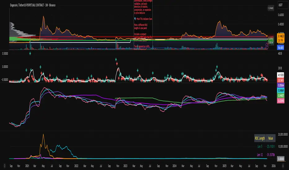
ROC x4 (Multi-Period Overlay) + Table📈 ROC x4 (Multi-Period Momentum Suite) + Compact Table
A clean, powerful momentum indicator that overlays four Rate-of-Change (ROC) periods inside a single pane — without needing to stack multiple separate indicators.
This script is designed for traders who use multi-timeframe momentum confirmation, trend strength validation, and early detection of rotation, compression, or expansion in price behavior.
🔍 What This Indicator Does
Plots 4 different ROC lengths in one panel
Includes a compact real-time ROC table that fits even in small panes
Tracks momentum shifts, trend acceleration, slowdowns, and regime transitions
Allows manual input for all 4 ROC lengths
Optional smoothing to reduce noise
Zero-line toggle for momentum direction clarity
Perfect for traders who want to monitor short-term, mid-term, and long-term ROC simultaneously.
EMA H/L 20-50 Table + RSI - KHALID ALADDIN🧾 Description
EMA H/L 20-50 Table + RSI — by Khalid Aladdin
A clean and minimal indicator designed for traders and analysts who prefer a quick glance at essential EMA values without any extra clutter on the chart.
📊 Features:
Displays precise values of EMA20 (High & Low) and EMA50 (High & Low) in a compact table below the chart.
Automatically updates values based on the current timeframe.
Includes RSI reading for momentum tracking.
Large, clear text with dark-theme friendly colors.
No lines or drawings — only a clean data panel.
✅ Perfect for:
Technical analysts, swing traders, and long-term investors who want an uncluttered view of trend levels and momentum strength.

USD Session 8FX - LDN & NY (TF-invariant, Live + Table)What it is
A USD strength/weakness meter for the London (08:00–08:45) or New York (15:30–16:00/16:15) session. It blends the movement of 8 markets—EURUSD, GBPUSD, AUDUSD, NZDUSD, USDCHF, USDCAD, USDJPY, XAUUSD—into one Score that is timeframe-invariant (it uses a 1-minute “boundary TF” under the hood so changing chart TF doesn’t change the math).
Core logic (simple)
During the chosen session window, it records each symbol’s start and live end prices, computes returns, optionally normalizes by ATR (volatility), applies your weights, and averages anti-USD (EUR/GBP/AUD/NZD/XAU) vs USD-base (CHF/CAD/JPY) groups.
The final Score is the normalized sum of weighted contributions:
Score > 0 → “USD Strong”
Score < 0 → “USD Weak”
At the session close it freezes (“Locked”) the results so you can review them later.
What you see
Main plot: the USD Score line (with a 0 baseline).
Optional lines: Anti-USD average vs USD-base average (post-normalization, pre-weights).
Session background shading (London silver, New York aqua).
Live table with:
Each symbol’s % change, its weight, and its contribution to the Score.
TOP badges for the two biggest drivers (by absolute contribution).
A Side column (only for the two TOPs) showing BUY/SELL aligned with the USD verdict (e.g., if USD Strong → SELL anti-USD pairs like EURUSD, BUY USD-base like USDCHF).
Verdict row with USD Strong/Weak, the Score value, the window text, and whether you’re LIVE / CLOSED / FROZEN.
Trade Gate panel:
Shows Verdict (USD Strong/Weak), Bias OK/weak (|Score| vs your threshold), Top-1/Top-2 VWAP checks, an overall GATE: OK/NO, and an Entry hint string (e.g., “SELL EURUSD, BUY USDCHF”) when conditions align.
VWAP “Trade Gate”
It confirms alignment between the USD bias and price vs VWAP for the top movers:
If USD Strong: anti-USD symbols should be below VWAP (short bias), USD-base symbols above VWAP (long bias).
If USD Weak: the opposite.
Gate = OK only if |Score| ≥ minAbsScore and at least one of the two TOP symbols is on the correct side of VWAP.
Tip: set vwapTF to an intraday value (“1”, “5”, “15”) for reliable VWAP on higher-TF charts.
Alerts
At session close: “USD Strong/Weak – session close”.
Live threshold: alerts when |Score| crosses your intraday threshold up/down.
Entry hint (Gate OK): triggers when the Gate flips from NO → OK inside the window.
If you create an alert of type “Any alert() function call”, you also get a dynamic message like:
ENTRY HINT • Hint: SELL EURUSD, BUY USDCHF
Key inputs you can tweak
Session: London vs New York; NY end time 16:00 or 16:15.
Timezone: default Europe/Tirane.
Boundary TF: default “1” (keeps the indicator TF-invariant).
minAbsScore: sensitivity threshold for “Bias OK”.
ATR normalization (len): stabilizes comparisons across different volatility regimes.
VWAP settings: toggle panel and set vwapTF.
How to use (playbook)
Choose the session (e.g., New York 15:30–16:15), keep Boundary TF = 1.
If you’re on a higher-TF chart, set vwapTF = "1" or "5".
Watch Score and Verdict; when |Score| ≥ minAbsScore, bias is meaningful.
Check Top-1/Top-2 and the Trade Gate:
If Gate = OK, use the Entry hint (e.g., “SELL EURUSD, BUY USDCHF”) as the aligned idea.
Use your own execution rules (e.g., structure, risk, stops) on the suggested symbols.
After close, review the Frozen table to validate behavior and refine thresholds/weights.
Notes & edge cases
If some markets are illiquid/holiday, a few returns may be na; the script handles that gracefully.
If ta.vwap is na on high TFs, the Gate will simply not confirm—set vwapTF intraday.
You can customize weights (e.g., reduce XAUUSD to -0.3 or similar) to suit your basket philosophy.
If you want, I can add toggles to show Side for all 8 symbols, or print a one-line summary (e.g., “USD Strong • Score 0.23 • Gate OK • SELL EURUSD, BUY USDCHF”) in the top-left of the pane.

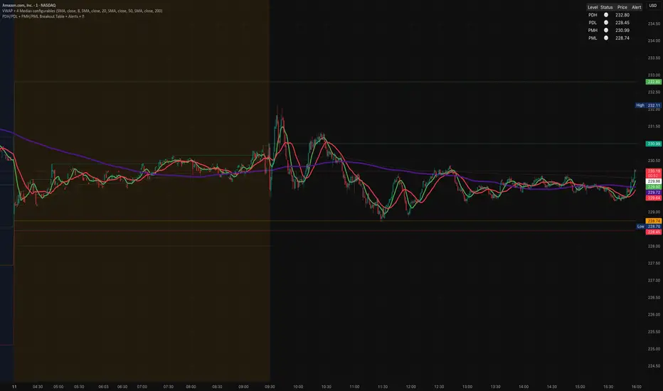
PDH/PDL + PMH/PML Breakout Table + Alerts + 🔔PDH/PDL now come exclusively from the previous day's RTH (9:30–4:00 PM ET) — they no longer include premarket. This avoids the confusion we encountered.
PMH/PML are calculated only during the premarket period (4:00–9:30 AM ET) of the current day.
Employment emojis: 🟢 (upward breakout for PDH/PMH), 🔴 (downward breakout for PDL/PML), ⚪ (no breakout).
The table displays three columns: Level | Status | Price. If you'd like the table to have a different size/position/color, just adjust it quickly.
Weinstein Stage Analyzer — Table Only (more padding)What it does
This indicator applies Stan Weinstein’s Stage Analysis (Stages 1–4) and presents the result in a clean, compact table only—no lines, labels, or overlays. It shows:
• Previous Stage
• Current Stage (with Early / Mature / Late tag)
• Duration (how long price has been in the current stage, in HTF bars)
• Sentiment (Bullish / Bearish / Balanced / Cautious, derived from stage & maturity)
Timeframe-aware logic
• Weekly charts: classic 30-period MA (Weinstein’s original 30-week concept).
• Daily & Intraday: computed on Daily 150 as a practical daily translation of the 30-week idea.
• Monthly: ~7-period MA (~30 weeks ≈ 7 months).
The stage classification itself is evaluated on this HTF context and then displayed on your active chart.
EMA/SMA toggle
Choose EMA (default) or SMA for the trend line used in stage detection.
How stages are decided (practical rules)
• Stage 2 (Advance): MA rising with price above an upper band.
• Stage 4 (Decline): MA falling with price below a lower band.
• Flat MA zones become Stage 1 (Base) or Stage 3 (Top) depending on the prior trend.
“Maturity” tags (Early/Mature/Late) come from run length and extension beyond the band.
Inputs you can tweak
• MA Type: EMA / SMA
• Price Band (±%) and Slope Threshold to tighten/loosen stage flips
• Maturity thresholds: min/max bars & late-extension %
Notes
• Duration is for the entire current stage (e.g., total time in Stage 4), not just the maturity slice.
• A Top Padding Rows input is included to nudge the table lower if it overlaps your OHLC readout.
Disclaimer
For educational use only. Not financial advice. Always confirm with your own analysis, risk management, and market context.

Trend Display Table (with Change Alerts)📌 Indicator: Trend Display Table (with Change Alerts)
This indicator helps identify trend direction based on a 15-minute 20 SMA compared against a 10 EMA applied to that SMA.
Trend Logic:
Bullish → 20 SMA crosses above 10 EMA (on SMA values)
Bearish → 20 SMA crosses below 10 EMA (on SMA values)
Neutral → No crossover (trend continues from previous state)
Display:
A compact trend table appears on the chart (top-right), showing the current trend with customizable colors, font size, and background.
Alerts:
Alerts are triggered only when the trend changes (from Bullish → Bearish or Bearish → Bullish).
This prevents repeated alerts on every bar.
✅ Useful for:
Confirming higher timeframe trend bias
Filtering trades in choppy markets
Getting notified instantly when the trend flips

RSI Z‑Score + TableRSI Z-Score + Table
This script calculates the Z-Score of the RSI (Relative Strength Index), which standardizes RSI based on its own recent history.
What It Shows:
RSI Z-Score = (Current RSI - Mean RSI) / Standard Deviation
This tells you how extreme the current RSI is compared to its historical values.
A table displays:
Current RSI
Rolling Mean
RSI Z-Score
How to Use:
Z-Score > +2 = Statistically overbought
Z-Score < -2 = Statistically oversold
Use it to time reversals or overextension in RSI behavior.
🔒 Based on rolling lookback window — fully customizable.
Author:
Tags: #RSI #ZScore #Momentum #StatisticalEdge #MeanReversion #Crypto

SG CBC Table - Full 10min & 2minBased on SG CBC Table has 10 min and 2 min CBC status and GC. Also customizable table colors of the background can be changed or made transparent. Indicator Updates every 10 minutes on a 10 minute chart and every 2 minutes on a 2 minute chart

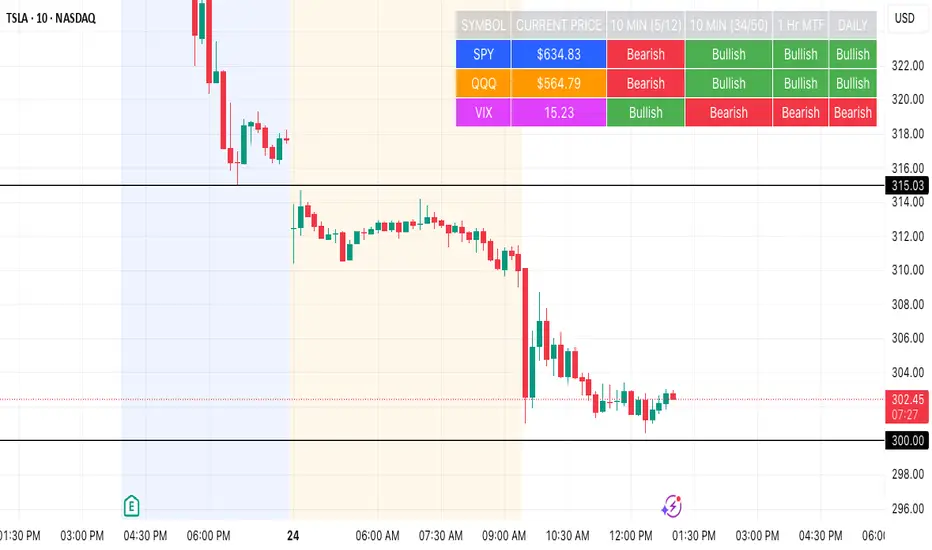
SPY, QQQ, VIX - Multi TF Trend Table***CURRENTLY IN BACKTESTING PHASE***
This TradingView script creates a real-time multi-timeframe trend status table for SPY, QQQ, and VIX using the Ripster-style EMA cloud logic.
🔍 What It Shows:
Current Price (1 Min): Live snapshot of each symbol.
10min Trend (5/12 EMA): Short-term momentum.
10min Trend (34/50 EMA): Intermediate-term direction.
1 Hour Trend: Higher timeframe trend.
Daily Trend: Long-term trend using 5/12 and 34/55 EMA alignment.
Each cell is color-coded:
✅ Green = Bullish
❌ Red = Bearish
Yellow can be used for neutral if customized.
⚙️ How It Works:
Uses request.security() to pull multi-timeframe EMA values for each symbol.
Compares fast/slow EMAs to determine bullish or bearish alignment.
The table is refreshed live and placed in a corner of your choice.
✅ Ideal For:
Trend traders using Ripster EMA clouds
SPY/QQQ/VIX correlation watchers
Traders seeking real-time trend clarity across multiple timeframes

SPY, QQQ, VIX Status TableBased on Ripster EMA and 1 hour MTF Clouds, this custom TradingView indicator displays a visual trend status table for SPY, QQQ, and VIX using multiple timeframes and EMA-based logic to be used on any stock ticker.
🔍 Key Features:
✅ Tracks 3 symbols: SPY, QQQ, and VIX
✅ Multiple trend conditions:
10-min (5/12 EMA) Ripster cloud trend
10-min (34/50 EMA) Ripster cloud trend
1-Hour Multi-Timeframe Ripster EMA trend
Daily open/close trend
✅ Color-coded trend strength:
🟩 Green = Bullish
🟥 Red = Bearish
🟨 Yellow = Sideways
✅ TO save screen space, customizations available:
Show/hide individual rows (SPY, QQQ, VIX)
Show/hide any trend column (10m, 1H MTF, Daily)
Change header/background colors and font color
Bold white top row for readability
✅ Auto-updating table appears on your chart, top-right
This tool is great for active traders looking to quickly scan short-term and longer-term momentum in key market instruments without having to go back and forth market charts.
PCR tableOverview
This indicator displays a multi-period table of forward-looking price projections. It combines normalized directional momentum (Positive Change Ratio, PCR) with volatility (ATR) and presents a forecast for upcoming time intervals, adjusted for your local UTC offset.
Concepts & Calculations
Positive Change Ratio (PCR):
((total positive change)/(total change)-0.5)*2, producing a value between –100 and +100.
Synthetic ATR: Calculates average true range over the same lookbacks to capture volatility.
PCR × ATR: Forms a volatility-weighted directional forecast, indicating expected move magnitude.
Future Price Projection: Adds PCR × ATR value to current close to estimate future price at each lookahead interval.
Table Layout
There are 12 forecast horizons—1× to 12× the chart timeframe (e.g., minutes, hours, days). Each row displays:
1. Future Time: Timestamp of each projection (adjustable via UTC offset)
2. PCR: Directional bias per period (–1 to +1)
3. PCR × ATR: E xpected move magnitude
4. Future Price: Close + (PCR × ATR)
High and low PCR×ATR rows are highlighted green for minimum value in the price forecast (buy signal) or red for maximum value in the price forecast (sell signal).
How to Use
1. Set UTC offset to your time zone for accurate future timestamps.
2. View PCR to assess bullish (positive) or bearish (negative) momentum.
3. Use PCR × ATR to estimate move strength and direction.
4. Reference Future Price for potential levels over upcoming intervals, and for buy and sell signals.
Limitations & Disclaimers
* This model uses linear extrapolation based on recent price behavior. It does not guarantee future prices.
* It uses only current bar data and no lookahead logic—compliant with Pine Script rules.
* Designed for analytical insight, not as an automated signal or trade executor.
* Best used on standard bar/candle charts (avoid non-standard types like Heikin‑Ashi or Renko).

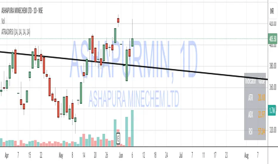
ATR, ADX, RSI TableATR, ADX & RSI Dashboard (Color-Coded)
Overview
This indicator provides a clean, all-in-one dashboard that displays the current values for three of the most popular technical indicators: Average True Range (ATR), Average Directional Index (ADX), and Relative Strength Index (RSI).
To make analysis faster and more intuitive, the values in the table are dynamically color-coded based on key thresholds. This allows you to get an immediate visual summary of market volatility, trend strength, and momentum without cluttering your main chart area.
Features
The indicator displays a simple table in the bottom-right corner of your chart with the following color logic:
ATR (Volatility): Measures the average volatility of an asset.
Green: Low Volatility (ATR is less than 3% of the current price).
Orange: Moderate Volatility (ATR is between 3% and 5%).
Red: High Volatility (ATR is greater than 5%).
ADX (Trend Strength): Measures the strength of the underlying trend, regardless of its direction.
Red: Weak or Non-Trending Market (ADX is below 20).
Orange: Developing or Neutral Trend (ADX is between 20 and 25).
Green: Strong Trend (ADX is above 25).
RSI (Momentum): Measures the speed and change of price movements to identify overbought or oversold conditions.
Green: Potentially Oversold (RSI is below 40).
Orange: Neutral/Normal Conditions (RSI is between 40 and 70).
Red: Potentially Overbought (RSI is above 70).
How to Use
This tool is perfect for traders who want a quick, at-a-glance understanding of the current market state. Instead of analyzing three separate indicators, you can use this dashboard to:
Quickly confirm if a strong trend is present before entering a trade.
Assess volatility to adjust your stop-loss and take-profit levels.
Instantly spot potential overbought or oversold conditions.
Customization
All input lengths for the ATR, ADX, and RSI are fully customizable in the indicator's settings menu, allowing you to tailor the calculations to your specific trading style and timeframe.
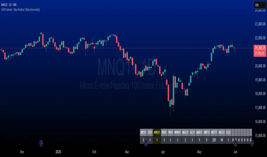
The LEAP Contest - Symbol & Max Position Table TrackerDescription:
This indicator tracks the maximum contracts allowed to be traded for TradingView’s *"The Leap"* Contest. It displays a horizontal table at the bottom right of your chart showing up to 20 symbols along with their maximum allowable open contract positions.
Use case:
Designed specifically for traders participating in *The Leap* Contest on TradingView.
Users need to enter the symbol and the maximum contracts allowed for that symbol in the settings menu for each new contest.
It provides a quick reference to ensure compliance with contest rules on maximum position sizes.
How it works:
The table shows two rows: the top row displays the symbol name, and the bottom row shows the max contract limit.
If the currently loaded chart symbol matches any symbol in the list, its text color changes to yellow .
Customization:
Symbols and limits must be updated in the indicator’s settings before each contest to reflect the current rules.
OBV Z-Score + Table📘 OBV Z-Score — Indicator Description
Overview
This indicator converts the On-Balance Volume (OBV) into a Z-Score oscillator, providing a normalized statistical view of volume flow strength relative to its recent history.
How It Works
OBV Calculation
The On-Balance Volume accumulates volume based on price direction, showing whether volume is flowing into or out of an asset.
Z-Score Transformation
The OBV values are normalized via Z-Score:
ini
Kopieren
Bearbeiten
Z = (OBV - Mean) / Standard Deviation
This reveals how unusually strong or weak volume momentum is compared to recent norms.
Smoothing
An optional moving average smoothing (SMA, EMA, VWMA, etc.) can be applied for cleaner signals.
Z-Score Table
A live Z-Score value is displayed in a table on the top-right of the indicator pane, clamped between +2 and -2:
+2 indicates unusually high positive volume momentum
-2 indicates unusually high negative volume momentum
How to Use It
Bullish Signal: Z-Score crossing above +1.5 or +2 signals strong buying volume pressure
Bearish Signal: Z-Score crossing below -1.5 or -2 signals strong selling volume pressure
Combine with Price Action: Use alongside price trends or other Z-Score indicators to improve decision making in SDCA or volume-based trading systems

RSI Z-Score + TableHow It Works
RSI Calculation
The standard RSI is computed over a user-defined period (default: 14), measuring the strength of recent price movements.
Z-Score Transformation
The RSI is then normalized using the Z-Score formula:
ini
Kopieren
Bearbeiten
Z = (RSI - Mean) / Standard Deviation
This highlights whether RSI is unusually high or low compared to its historical behavior.
Smoothing
An optional EMA is applied to the Z-Score for smoother and more reliable signals (default: 10-period smoothing).
Z-Score Table
A real-time value of the RSI Z-Score is displayed in a table in the top-right of the indicator pane.
The value is clamped between +2 and -2
+2 aligns with strong overbought RSI conditions
-2 aligns with strong oversold RSI conditions
How to Use It
Buy Signal Potential: When the Z-Score drops below -1.5 or -2 → statistically oversold RSI
Sell Signal Potential: When the Z-Score rises above +1.5 or +2 → statistically overbought RSI
Use in Confluence: Combine with price action, trend filters, or other Z-Score indicators (e.g. OBV, VWAP, VIX) for SDCA or mean-reversion strategies

VWAP Z-Score Oscillator + Scaled TableVWAP Z-Score Oscillator + Scaled Table
This indicator calculates the Z-Score of the VWAP (Volume Weighted Average Price) based on your chosen source price and reset period (Session, Week, Month, Quarter, or Year).
The Z-Score represents how many standard deviations the current price is from the VWAP, visualized as an oscillator oscillating between ±3 sigma levels. The indicator also features three standard deviation bands for easy reference.
To enhance readability, a scaled Z-Score is displayed in a clean, minimalistic table on the top right of the indicator panel. This score is linearly capped between -2 and +2, mapping the raw Z-Score values with limits at ±3 sigma for clarity and quick assessment.
Use this tool to identify extreme deviations from the VWAP, which may signal potential reversals or continuation of price trends.

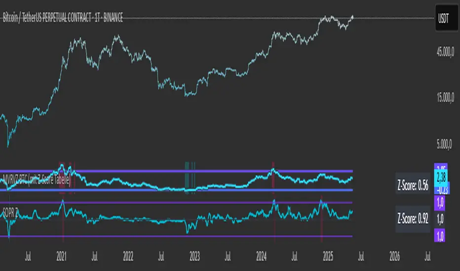
SOPR with Z-Score Table📊 Glassnode SOPR with Dynamic Z-Score Table
ℹ️ Powered by Glassnode On-Chain Metrics
📈 Description:
This indicator visualizes the Spent Output Profit Ratio (SOPR) for major cryptocurrencies — Bitcoin, Ethereum, and Litecoin — along with a dynamically normalized Z-Score. SOPR is a key on-chain metric that reflects whether coins moved on-chain are being sold at a profit or a loss.
🔍 SOPR is calculated using Glassnode’s entity-adjusted SOPR feed, and a custom SMA is applied to smooth the signal. The normalized Z-Score helps identify market sentiment extremes by scaling SOPR relative to its historical context.
📊 Features:
Selectable cryptocurrency: Bitcoin, Ethereum, or Litecoin
SOPR smoothed by user-defined SMA (default: 10 periods)
Upper & lower bounds (±4%) for SOPR, shown as red/green lines
Background highlighting when SOPR moves outside normal range
Normalized Z-Score scaled between –2 and +2
Live Z-Score display in a compact top-right table
🧮 Calculations:
SOPR data is sourced daily from Glassnode:
Bitcoin: XTVCBTC_SOPR
Ethereum: XTVCETH_SOPR
Litecoin: XTVCLTC_SOPR
Z-Score is calculated as:
SMA of SOPR over zscore_length periods
Standard deviation of SOPR
Z-Score = (SOPR – mean) / standard deviation
Z-Score is clamped between –2 and +2 for visual consistency
🎯 Interpretation:
SOPR > 1 implies coins are sold in profit
SOPR < 1 suggests coins are sold at a loss
When SOPR is significantly above or below its recent range (e.g., +4% or –4%), it may signal overheating or capitulation
The Z-Score contextualizes how extreme the current SOPR is relative to history
📌 Notes:
Best viewed on daily charts
Works across selected assets (BTC, ETH, LTC)
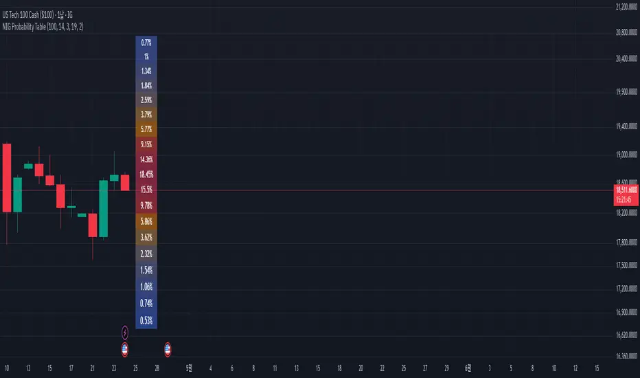
NIG Probability TableNormal-Inverse Gaussian Probability Table
This indicator implements the Normal-Inverse Gaussian (NIG) distribution to estimate the likelihood of future price based on recent market behavior.
📊 Key Features:
- Estimates the parameters (α: tail heaviness, β: skewness, δ: scale, μ: location)
of the NIG distribution using a sliding window over log returns.
- Uses a numerically approximated version of the modified Bessel function (K₁)
to calculate the NIG probability density function (PDF).
- Normalizes the total probability across all bins to ensure the values are interpretable.
- Displays a dynamic probability table showing the chance of future returns falling into each bin.
⚠️ Notes:
- This is a real-time approximation. The Bessel function and posterior inference are simplified.
- Tail probabilities and shape parameters are sensitive to the window size and input settings.
- Useful for risk analysis, option overlays, and strategy filters.
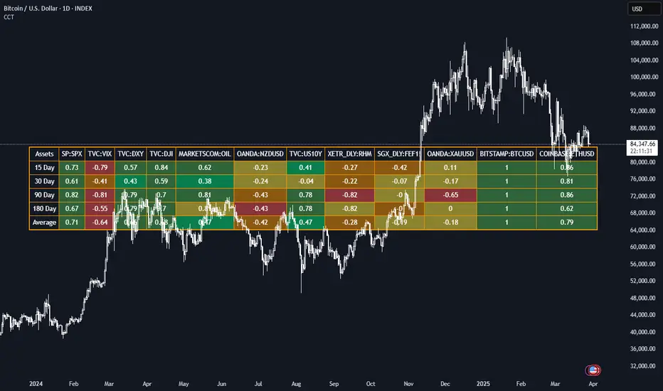
Correlation Coefficient TableThis Pine Script generates a dynamic table for analyzing how multiple assets correlate with a chosen benchmark (e.g., NZ50G). Users can input up to 12 asset symbols, customize the benchmark, and define the beta calculation periods (e.g., 15, 30, 90, 180 days). The script calculates Correlation values for each asset over these periods and computes the average beta for better insights.
The table includes:
Asset symbols: Displayed in the first row.
Correlation values: Calculated for each defined period and displayed in subsequent columns.
Average Correlation: Presented in the final column as an overall measure of correlation strength.
Color coding: Background colors indicate beta magnitude (green for high positive beta, yellow for near-neutral beta, red for negative beta).
ATR & PTR TableThe ATR & PTR Table Indicator displays a dynamic table that provides Average True Range (measures market volatility over 1D, 1W, and 1M timeframes), Price trading range (difference between the high and low prices over the same periods) & percentage of the typical range that has been traded. This indicator will help traders identify potential breakout zones and assess volatility across multiple timeframes.
This had been optimized to show ATR and PTR on every time frame. The (1D) represents ATR on whatever timeframe you are currently on.
