Ciclos


Adaptive MVRV & RSI Strategy V6 (Dynamic Thresholds)Strategy Explanation
This is an advanced Dollar-Cost Averaging (DCA) strategy for Bitcoin that aims to adapt to long-term market cycles and changing volatility. Instead of relying on fixed buy/sell signals, it uses a dynamic, weighted approach based on a combination of on-chain data and classic momentum.
Core Components:
Dual-Indicator Signal: The strategy combines two powerful indicators for a more robust signal:
MVRV Ratio: An on-chain metric to identify when Bitcoin is fundamentally over or undervalued relative to its historical cost basis.
Weekly RSI: A classic momentum indicator to gauge long-term market strength and identify overbought/oversold conditions.
Dynamic, Self-Adjusting Thresholds: The core innovation of this strategy is that it avoids fixed thresholds (e.g., "sell when RSI is 70"). Instead, the buy and sell zones are dynamically calculated based on a long-term (2-year) moving average and standard deviation of each indicator. This allows the strategy to automatically adapt to Bitcoin's decreasing volatility and changing market structure over time.
Weighted DCA (Scaling In & Out): The strategy doesn't just buy or sell a fixed amount. The size of its trades is scaled based on conviction:
Buying: As the MVRV and RSI fall deeper into their "undervalued" zones, the percentage of available cash used for each purchase increases.
Selling: As the indicators rise further into "overvalued" territory, the percentage of the current position sold also increases.
This creates an adaptive system that systematically accumulates during periods of fear and distributes during periods of euphoria, with the intensity of its actions directly tied to the extremity of market conditions.

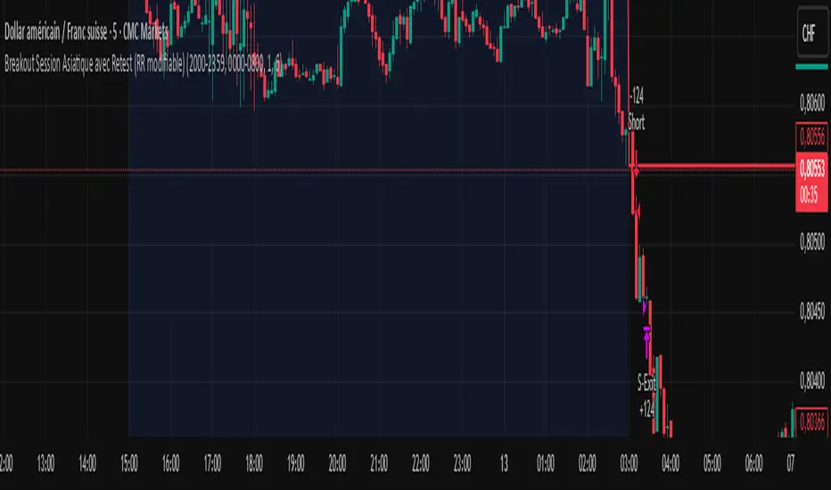
Breakout asia USD/CHF1 — Customizable Parameters
sess1 & sess2: The two time ranges that define the Asian session (e.g., 20:00–23:59 and 00:00–08:00).
Important: format is HHMM-HHMM.
rr: The risk/reward ratio (default = 3.0, meaning TP = 3× risk size).
onePerSess: Toggle to allow only one trade per Asian session or multiple.
bufTicks: Extra margin for the SL beyond the signal candle.
2 — Detecting the Asian Session
The script checks if the candle’s time is inside the first range (sess1) or inside the second range (sess2).
While inside the Asian session, it updates the current high and low.
When the session ends, it locks in these levels as rangeHigh and rangeLow.
3 — Step 1: Detecting the Initial Breakout
Bullish breakout → close above rangeHigh → flag breakoutUp is set to true.
Bearish breakout → close below rangeLow → flag breakoutDown is set to true.
No trade yet — this is just the breakout signal.
4 — Step 2: Waiting for the Retest
If a bullish breakout occurred, wait for the price to return to or slightly below rangeHigh and then close back above it.
If a bearish breakout occurred, wait for the price to return to or slightly above rangeLow and then close back below it.
5 — Entry & Exit
When the retest is confirmed:
strategy.entry() is triggered.
SL = behind the retest confirmation candle (with optional bufTicks margin).
TP = entry price ± RR × risk size.
If onePerSess is enabled, no further trades happen until the next Asian session.
6 — Chart Display
Green line = locked Asian session high.
Red line = locked Asian session low.
Light blue background = active Asian session hours.
Trade entries are shown on the chart when retests occur.
Nova Futures PRO (SAFE v6) — HTF + Choppiness + CooldownNova Futures PRO (SAFE v6) — HTF + Choppiness + Cooldown

Estrategia de NY ORB por CPThis strategy marks the New York market opening range during the first 15 minutes and confirms a buy or sell entry once the price returns and retests that range. It’s designed to capture trades of 60 points or more after the range has been retested. I suggest complementing the strategy with an indicator that highlights FVGs (Fair Value Gaps) or order blocks to better understand what price is doing and where it’s heading.
esta estrategia te marca el rango de apertura del mercado de ny de los primeros 15 minutos y te confirma entrada en venta o compra una vez que el precio regrese y retestee el rango. esta diseñada para tener trades de 60 puntos o mas una vez que el rango sea retesteado. sugiero acompañar la estrategia con algun indicador que marque fvg o order blocks para tener una mejor de lo que el precio esta haciendo y hacia donde se dirige.

CP Strat ORBnew york opening range breakout and retest allows you to enter a trade with a better clarity if the price comes back and retest the range

ORB 15m – First 15min Breakout (Long/Short)ORB 15m – First 15min Breakout (Long/Short)
Apply on SPY, great returns

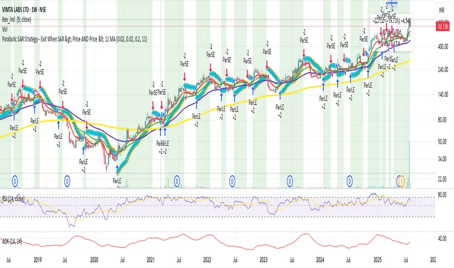
MomentumSync-PSAR: RSI·ADX Filtered 3-Tier Exit StrategyTriSAR-E3 is a precision swing trading strategy designed to capitalize on early trend reversals using a Triple Confirmation Model. It triggers entries based on an early Parabolic SAR bullish flip, supported by RSI strength and ADX trend confirmation, ensuring momentum-backed participation.
Exits are tactically managed through a 3-step staged exit after a PSAR bearish reversal is detected, allowing gradual profit booking and downside protection.
This balanced approach captures trend moves early while intelligently scaling out, making it suitable for directional traders seeking both agility and control.

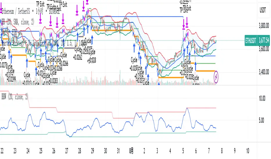
Martin Strategy - No Loss Exit v3Martin Strategy1.0 Martin Strategy1.0 Martin Strategy1.0 Martin Strategy1.0 Martin Strategy1.0 Martin Strategy1.0
Parabolic SAR with Early Buy & MA-Based Exit Strategy📝 Strategy Description (Max SEO Impact)
This advanced Parabolic SAR-based trading strategy is designed to capture early trend reversals and exit intelligently using a dynamic moving average filter. It enters long trades when a PSAR reversal occurs, and exits only when the PSAR moves above price and the price falls below the 11-period SMA, helping avoid premature exits during volatile swings.
📌 Features:
• Custom Parabolic SAR calculation for refined trend tracking
• Background highlights during buy zones (SAR below price)
• Exit signals only when trend weakens (PSAR above + price under SMA)
• Red flag plotted on chart at exit bars for clear visual identification
• Works on all timeframes and instruments
Ideal for swing traders, trend followers, and strategy testers looking for smart PSAR-based entries with smoother exits.

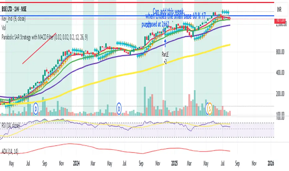
Parabolic SAR Strategy with MACD Confirmation & Trend Zone Highl📝 Description (SEO + Follower-Friendly):
🚀 Powerful Trend Strategy Using Parabolic SAR + MACD
This advanced Pine Script combines the classic Parabolic SAR trend-following system with MACD crossover confirmation, improving entry precision and filtering out false signals. The script also features:
✅ Dynamic trend zone background highlighting when SAR is below price
✅ MACD filter ensures trades align with market momentum
✅ Custom SAR logic with adaptive acceleration
✅ Clean visual SAR plots for easy trend tracking
✅ Fully backtestable with strategy.entry logic
🔎 Ideal for traders seeking early trend entries, momentum confirmation, and visual clarity.
📈 Works on all timeframes and pairs — perfect for swing traders, scalpers, and crypto enthusiasts.
💡 Use it as a base strategy or combine with your favorite indicators.
❤️ If you find this helpful, don't forget to like, comment, and follow for more premium strategies!
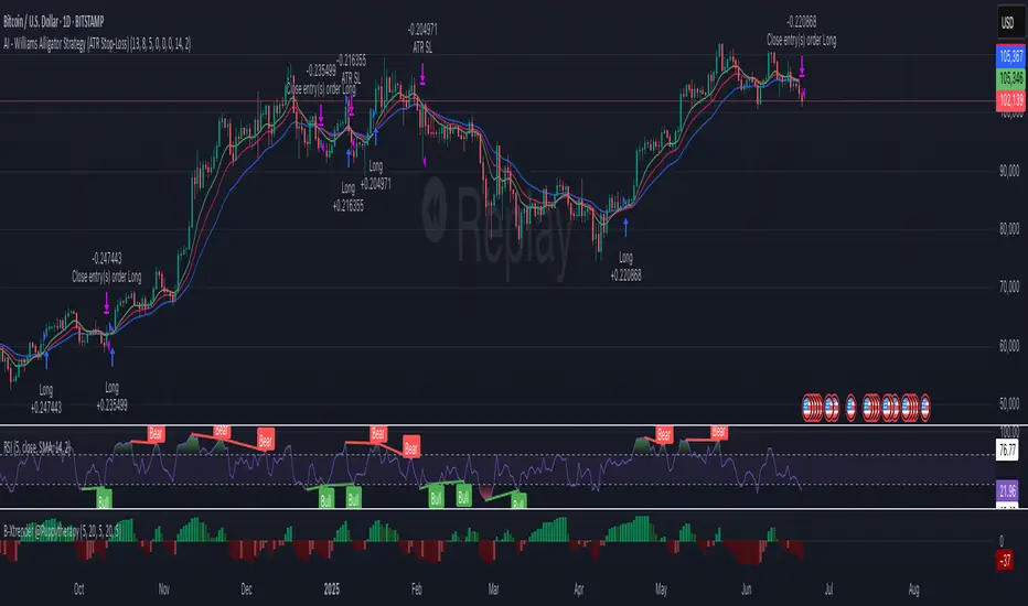
AI - Williams Alligator Strategy (ATR Stop-Loss) AlertsAI - Williams Alligator Strategy (ATR Stop-Loss) with Alerts
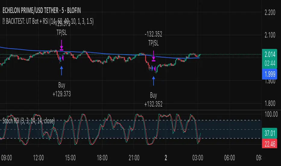
✅ BACKTEST: UT Bot + RSIRSI levels widened (60/40) — more signals.
Removed ATR volatility filter (to let trades fire).
Added inputs for TP and SL using ATR — fully dynamic.
Cleaned up conditions to ensure alignment with market structure.
Opening-Range BreakoutNote: Default trading date range looks mediocre. Set date range to "Entire History" to see full effect of the strategy. 50.91% profitable trades, 1.178 profit factor, steady profits and limited drawdown. Total P&L: $154,141.18, Max Drawdown: $18,624.36. High R^2
█ Overview
The Opening-Range Breakout strategy is a mechanical, session‑based day‑trading system designed to capture the initial burst of directional momentum immediately following the market open. It defines a user‑configurable “opening range” window, measures its high and low boundaries, then places breakout stop orders at those levels once the range closes. Built‑in filters on minimum range width, reward‑to‑risk ratios, and optional reversal logic help refine entries and manage risk dynamically.
█ How It Works
Opening‑Range Formation
Between 9:30–10:15 AM ET (configurable), the script tracks the highest high and lowest low to form the day’s opening range box.
On the first bar after the range window closes, the range high (OR_high) and low (OR_low) are “locked in.”
Range‑Width Filter
To avoid false breakouts in low‑volatility mornings, the range must be at least X% of the current price (default 0.35%).
If the measured opening-range width < minimum threshold, no orders are placed that day.
Entry & Order Placement
Long: a stop‑buy order at the opening‑range high.
Short: a stop‑sell order at the opening‑range low.
Only one side can trigger (or both if reverse logic is enabled after a losing trade).
Risk Management
Once triggered, each trade uses an ATR‑style stop-loss defined as a percentage retracement of the range (default 50% of range width).
Profit target is set at a configurable Reward/Risk Ratio (default 1.1×).
Optional: Reverse on Stop‑Loss – if the initial breakout loses, immediately reverse into the opposite side on the same day.
Session Exit
Any open positions are closed at the end of the regular trading day (default 3:45 PM ET window end, with hard flat at session close).
Visual cues are provided via green (range high) and red (range low) step‑line plots directly on the chart, allowing you to see the range box and breakout triggers in real time.
█ Why It Works
Early Momentum Capture: The first 15 – 60 minutes of trading encapsulate overnight news digestion and institutional order flow, creating a well‑defined volatility “range.”
Mechanical Discipline: Clear, rule‑based entries and exits remove emotional guesswork, ensuring consistency.
Volatility Filtering: By requiring a minimum range width, the system avoids choppy, low‑range days where false breakouts are common.
Dynamic Sizing: Stops and targets scale with the opening range, adapting automatically to each day’s volatility environment.
█ How to Use
Set Your Instruments & Timeframe
-Apply to any futures contract on a 1‑ to 5‑minute chart.
-Ensure chart timezone is set to America/New_York.
Configure Inputs
-Opening‑Range Window: e.g. “0930-1015” for a 45‑minute range.
-Min. OR Width (%): e.g. 0.35 for 0.35% of current price.
-Reward/Risk Ratio: e.g. 1.1 for a modest profit target above your stop.
-Max OR Retracement %: e.g. 50 to set stop at 50% of range width.
-One Trade Per Day: toggle to limit to a single breakout.
-Reverse on Stop Loss: toggle to flip direction after a losing breakout.
Monitor the Chart
-Watch the green and red range boundaries form during the session open.
-Orders will automatically submit on the first bar after the range window closes, conditioned on your filters.
Review & Adjust
-Backtest across multiple months to validate performance on your preferred contract.
-Tweak range duration, minimum width, and R/R multiple to fit your risk tolerance and desired win‑rate vs. expectancy balance.
█ Settings Reference
Input Defaults
Opening‑Range Window - Time window to form OR (HHMM-HHMM) - 0930–1015
Regular Trading Day - Full session for EOD flat (HHMM-HHMM) - 0930–1545
Min. OR Width (%) - Minimum OR size as % of close to trigger orders - 0.35
Reward/Risk Ratio - Profit target multiple of stop‑loss distance - 1.1
Max OR Retracement (%) - % of OR width to use as stop‑loss distance - 50
One Trade Per Day - Limit to a single breakout order per day - false
Reverse on Stop Loss - Reverse direction immediately after a losing trade - true
Disclaimer
This strategy description and any accompanying code are provided for educational purposes only and do not constitute financial advice or a solicitation to trade. Futures trading involves substantial risk, including possible loss of capital. Past performance is not indicative of future results. Traders should assess their own risk tolerance and conduct thorough backtesting and forward-testing before committing real capital.

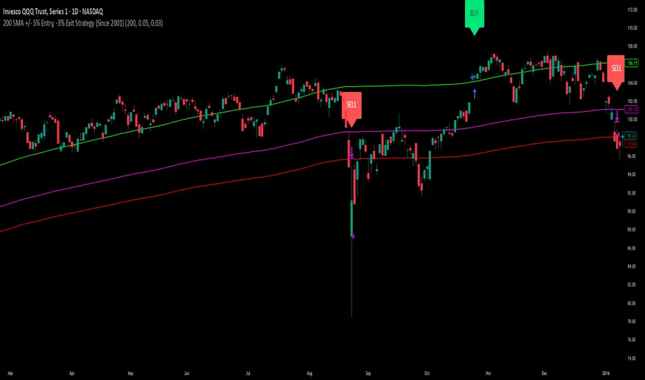
200 SMA (5%/-3% Buffer) for SPY & QQQ In my testing TQQQ is an absolute monster of an ETF that performs extremely well even from a buy and hold standpoint over long periods of time, its largest drawback is the massive drawdown exposure that it faces which can be easily sidestepped with this strategy.
This strategy is meant to basically abuse TQQQ's insane outperformance while augmenting the typical 200SMA strategy in a way that uses all of its strengths while avoiding getting whipsawed in sideways markets.
The strategy BUYS when price crosses 5% over the 200SMA and then SELLS when price drops 3% below the 200SMA. Between trades I'll be parking my entire account in SGOV.
So maximizing profit while minimizing risk.
You use the strategy based off of QQQ and then make the trades on TQQQ when it tells you to BUY/SELL.
Here are some reasons why I will be using this strategy:
Simple emotionless BUY and SELL signals where I don't care who the president is, what is happening in the world, who is bombing who, who the leadership team is, no attachment to individual companies and diversified across the NASDAQ.
~85% win percentage and when it does lose the loses are nothing compared to the wins and after a loss you're basically set up for a massive win in the next trade.
Max drawdown of around 53% when using TQQQ
You benefit massively when the market is doing well and when there is a recession you basically sit in SGOV for a year and then are set up for a monster recovery with a clear easy BUY signal. So as long as you're patient you win regardless of what happens.
The trades are often very long term resulting in you taking advantage of Long Term Capital Gains tax advantage which could mean saving up to 15-20% in taxes.
With only a few trades you can spend time doing other stuff and don't have to track or pay attention to anything that is happening.
Simple, easy, and massively profitable.
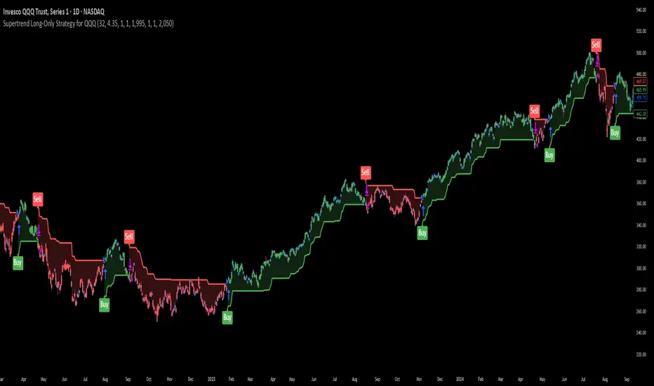
Supertrend Long-Only Strategy for QQQThis strategy is meant to use Micro Momentum to give good Buy and Sell signals in trending markets
BB + RSI Strategy Optimized✅ Pine Script Version 5
✅ Complete Strategy: Long + Short
✅ Automatic Entry and Exit
✅ Visual Signals: Buy/Sell, Short/Cover
✅ Trailing Take Profit
✅ Progressive

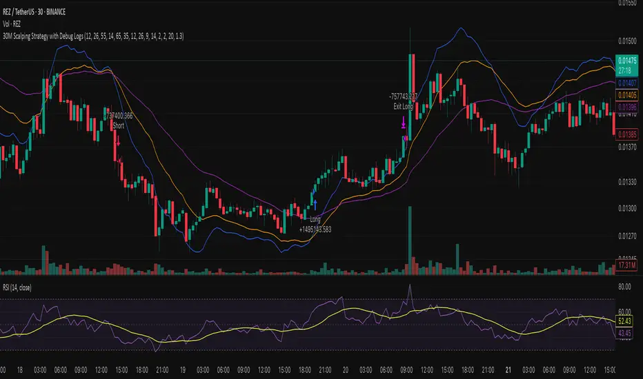
30M Scalping Strategy with Debug LogsWhat’s changed
Spot‑only: all short logic removed—only long entries and exits are generated.
Logging: uses log.info() to send entry/exit details (timestamp, price, ATR, RSI) to the Pine Logs console.
Clean & concise: core scalp logic (EMAs, RSI, MACD, volume, ATR SL/TP) remains intact.