Short Volume Weighted Trend Band VTrendThe Short Volume Weighted Trend band, combined with the custom supertrend and barcolor, which changes according to price going above or below the bollinger band basis line. Is designed for you to identify the high time frame trend, and take short to long term entries.
The short volume band in green, acts as dynamic support and resistance, and price respects this quite well. I find it great for taking entries off and placing stops below or above depending on the position being taken.
It really helps identify when price is actually changing trend. The barcolor change assists in acting as confluence for this.
Included is a custom supertrend, which is better at 1h timeframe an above. And daily open levels only, as i find the daily key to take trades off when i am scalping on an intraday basis.
The reversal calculations are based off candle close types, these are 'R' either in black or red. The difference in black and red is a type only, and means no significance between the two.
Timeframes I like using on this script, 2H, 1H, 30min, 25min, 15min
Bands

Root mean squared error range (RMSER)Similarly to Bollinger bands, the RMSER gives a support and resistance areas for the trading price. Unlike bollinger bands, which use standard deviation, this support and resistance is calculated with 2 * the root mean squared error away from the moving average. This works very well with indices, like $SPX, and prices only fall outside the range during black swan events like the 2020 crash.

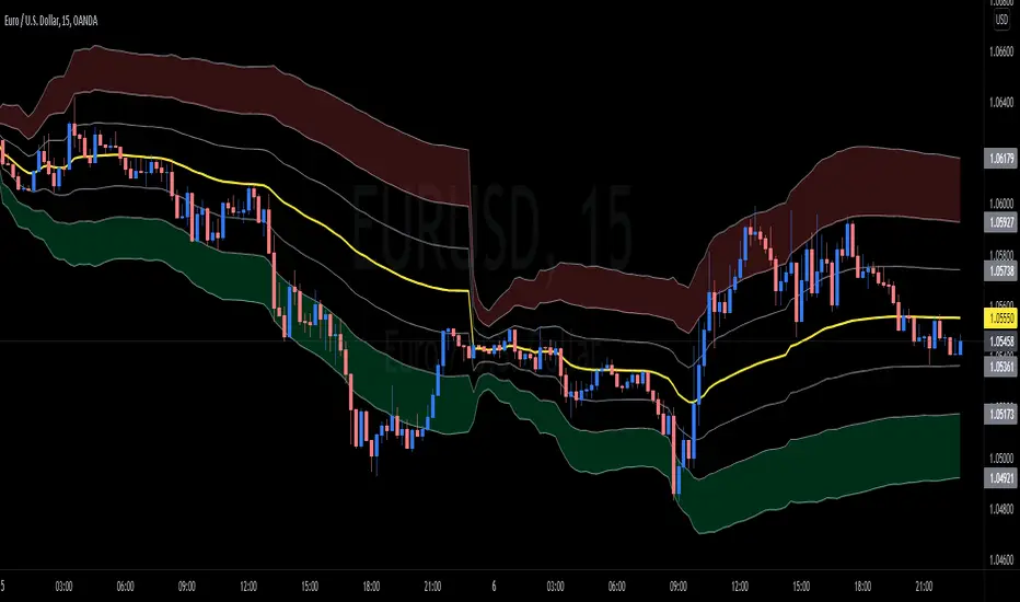
wnG - VWAP MOD Modified version of VWAP :
Classic VWAP with 6 levels based on the Average True Range to identify the distance and distribution of the prices around the VWAP.
There are 2 calcul methodologies for the bands
- Last 24 Hours Average True Range
- Progressive Average True Range starting from 00:00
As prices tend to move around the VWAP level, favor LONG positions in the GREEN ZONE (and SHORT in the RED ZONE).
How to use it :
Avoid taking long position when price is in the RED ZONE
Avoid taking short position when price is in the GREEN ZONE
==> Adjust the settings depending on your timeframe and asset
ATR BandsIn many strategies, it's quite common to use a scaled ATR to help define a stop-loss, and it's not uncommon to use it for take-profit targets as well. While it's possible to use the built-in ATR indicator and manually calculate the offset value, we felt this wasn't particularly intuitive or efficient, and could lead to the potential for miscalculations. And while there are quite a few indicators that plot ATR bands in some form or another already on TV, we could not find one that actually performed the exact way that we wanted. They all had at least one of the following gaps:
The ATR offset was not configurable (usually hard-coded to be based off the high or low, while we generally prefer to use close)
It would only print a single band (either the upper or lower), which would require the same indicator to be added twice
The ATR scaling factor was either not configurable or only stepped in whole numbers (often time fractional factors like 1.5 yield better results)
To that end, we took to making this enhanced version to meet all of the above requirements. While we were doing so, we decided to take this opportunity to also make some non-functional enhancements as well:
Updated the indicator to the most recent version of Pine
Updated the indicator definition to allow alternate (non-chart) timeframe usage
Made the input types explicitly defined to improve consistency
Updated the inputs with appropriate minimum values and step sizes where appropriate
Separated settings into logical groups
Added helptext to the indicator settings noting usage and common settings values
Explicitly titled the on-chart plots of the ATR bands so that they can more easily be identified and referenced in other indicators/scripts, as well as the Data Window
Food for thought : When looking at some of the behaviors of these ATR bands, you can see that when price first levels out, you can draw a "consolidation zone" from the first peak of the upper ATR band to the first valley of the lower ATR band that price will generally respect. Look for price to break and close outside of that zone. When that happens, price will usually (but not always) make a notable move in that direction, which can be used as either a potential trigger or as an additional confluence with other indicators/price action.
Finally, while we have made what we feel are some noteworthy updates and enhancements to this indicator, and have every intention of continuing to do so as we find worthy opportunities for enhancement, credit is still due to the original author: AlexanderTeaH

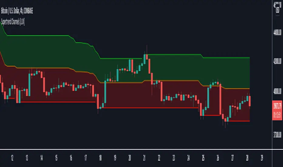
Supertrend Channels [LuxAlgo]The Supertrend is one of the most used indicators by traders when it comes to determining whether the market is up-trending or down-trending.
This indicator is displayed as a trailing stop, showing a lower monotonic extremity during up-trends and an upper monotonic extremity during down-trends. Today we propose a channel indicator based on the Supertrend trailing stop using trailing maximas/minimas.
Settings
Length: Atr length used by the Supertrend indicator.
Mult: Multiplicative factor for the Atr used by the Supertrend indicator.
Usage
The ability of the indicator to show an up-trend or down-trend is the same as the Supertrend, with rising channels when an up-trend is detected by the Supertrend and declining channels when a down-trend is detected by the Supertrend.
The look of the channels can remind of the Donchian channels indicator, and as such a similar usage can be appropriate. The extremities can for example be used as supports and resistances.
Additionally, the channel's average can be used to filter out noisy variations in the price while keeping a good distance from the price.
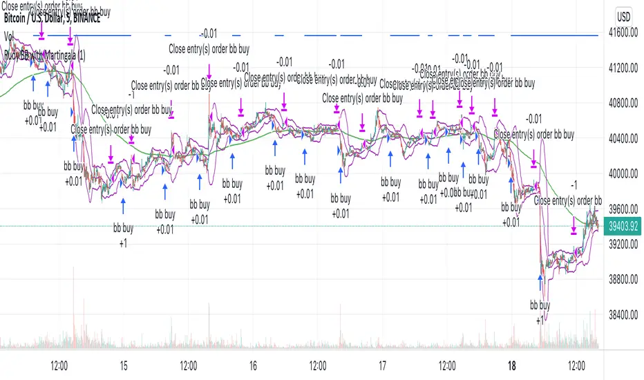
Rudy's BB with MartingaleMy first strategy script that uses Bollinger Bands and Martingale to increase contract size after negative profit.
Deadly Trio V2.0Overview:
This is a fully featured StochRSI, RSI & Bollinger Bands customisable indicator with custom conditions and alerts that can be taken advantage of using automated solutions such as Autoview, 3Commas or using it alongside/testing BUY/SELL conditions against your favourite markets to maximise gains. Finally you can use this a standalone manual general purpose signals indicator to scalp or accumulate your chosen market.
Time Frame:
This Indicator is specially customize for 5min time frame, but you can use it on Higher Time Frames as well, such as 15min, 1hr, 4hr and 1Day.
How to Use:
Long Position:
When the RSI is in Oversold (below 30) in 5min time frame, and Deadly Trio shows BUY Signal, then enter in the trade with long position.
Take Profit for Long Position:
When the candle touches the middle line (White Line) then it will be consider as the Target 1 Hit. When the candle touches the Upper Band then it will be consider as the Target-2 Hit. Always book some profit on Target-1. To play safe, you can close your trade in profit when the Target-1 Hit.
Short Position:
When the RSI is in Overbought (above 70) in 5min time frame and Deadly Trio Indictor shows SELL Signal, then enter in the trade with short position.
Take Profit for Short Position:
When the candle touches the middle line (White Line) then it will be consider as the Target 1 Hit. When the candle touches the Lower Band then it will be consider as the Target-2 Hit. Always book some profit on Target-1. To play safe, you can close your trade in profit when the Target-1 Hit.
How to do DCA (Dollar Cost Averaging):
If you want to maximize your profit, or you want to exit your trade always in profit then DCA (Dollar Cost Averaging) is very necessory. For DCA, always buy in parts. If you are in Long Position and another BUY signals appears on Deadly Trio, then Buy some more as per your financial conditions. Same condition apply for Short Position when SELL signal appears.
When to EXIT the Trade:
If you are in Long Position/Short Position and SELL / BUY Signal appears on the candle then close your Long Position/Short Position. You can also use this condition as a STOP LOSS.

Mobo BandsThis indicator is the Mobo Bands (Momentum Breakout Bands). These bands are bollinger bands that have an adjusted standard deviation. There are Buy signals when it has momentum breakouts above the bands for moves to the upside and Sell signals when it has momentum breakouts below the bands for moves to the downside. The bands simply suggest that all markets have periods of chop which we all know to be true. While the price is inside the bands it is said to be trendless. Once the breakouts happen you can take trades in the breakout direction. I like to use these to swing trade options on the hourly timeframe but the bands should work on most instruments and timeframes. I like to use it to take swings on SPY on the 1 hour chart for entries and use the Daily chart for trend confirmation.
Weighted Standard Deviation BandsLinearly weighted standard deviations over linearly weighted mean.
The rationale of the study can be deduced from my latest publications where I go deeper into explaining the benefits of linear weighting, but in short, I can remind that by using linear weighting we are able to increase the information gain by communicating the sequential nature of time series to the calculations via linear weighting.
Note, that multiplier parameters can take both negative and positive values resulting in ability to have, for example, 1st and 6th weighted standard deviations higher than the weighted mean.
Despite the modification of the classic standard deviation formula, I assume that mathematical qualities of standard deviation will hold due to the fact we can alternately weight the window itself, and then apply the classic standard deviation over the weighted window. In both cases, the results will be the same.
Aight that was too formal, but your short strangles should be happy
Here is it, for you

Anchored TWAP with StDev Bands [MrShadow]TWAP with:
- Anchoring: Custom, Day, Week, Month, Quarter, Year (custom anchoring can be selected by dragging a vertical line through the chart)
- Standard Devation Bands
- Auto-coloring depending on the trend
Volatility ChannelThis script is based on an idea I have had for bands that react better to crypto volatility. It calculates a Donchian Channel, SMMA-Smoothed True Range, Bollinger Bands (standard deviation), and a Keltner Channel (average true range) and averages the components to construct its bands/envelopes. This way, hopefully band touches are a more reliable indicator of a temporary bottom, and so on. Secondary coloring for strength of trend is given as a gradient based on RSI.

BBands ChannelsBased on the Bollinger Bands system. This shows outer channels to the bollinger bands .

BEAM DCA Strategy MonthlyThis strategy is based on BEAM bands for BTC. The space between the original BEAM bands is broken up into 10 bands representing levels of risk for investing fresh capital.
The strategy will buy bitcoin when the price is in the bottom 5 bands, increasing the amount investmented as the price approaches the 1400 D SMA.
The strategy will limit sell bitcoin when the price is in the top 5 bands, increasing the amount sold as the price approaches the upper BEAM band.
Best used on Daily timeframe and on a chart with history of price data, i.e. INDEX:BTCUSD or BITSTAMP:BTCUSD
To use the strategy:
Set start date
Set day of month to invest
Set the maximum amount to be invested on any given month
Toggle buy/sell orders
Observe the backtest
You can see how the strategy backtests via the information boxes in the bottom right.
There is also functionality to adjust the bands for diminishing returns. Note, this should be used with great skepticism, as the adjustments were made by simple function fitting and not rigorous statistical processes.
That about sums it up! As you can see, even with just a small amount of capital invested at regular intervals can lead to huge realised gains using this version of BEAM bands!

Flat Detect By Bollinger BandsThis simple script indicate the potential flat market zones, calculated based on the Bollinger Bands width.
It's showing the Bollinger Bands in red when the market is detected as flat.
You can adjust the Width Threshold with precision on the inputs settings.
Enjoy :)

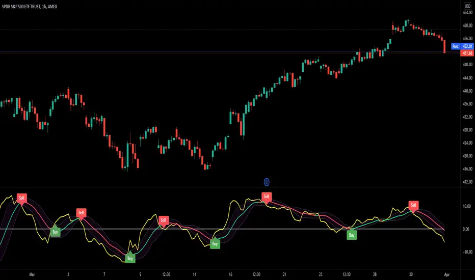
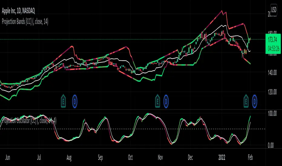
Projection Oscillator [CC]The Projection Oscillator was created by Mel Widner (Stocks and Commodities Jul 1995) and this is another hidden gem that is of course a great complementary indicator to my previous Projection Bands . I would recommend to use both on the same chart so you get the full array of information. This indicator tells you where the current price falls between the bands and the higher the oscillator is, the closer the price is to the upper band and vice versa. Now since the price never falls outside of the bands, the indicator is limited from 0 to 100. You will notice that with this indicator it gives even earlier signals than the Projection Bands so a very useful indicator indeed. I have included strong buy and sell signals in addition to normal ones so strong signals are darker in color and normal signals are lighter in color. Buy when the line turns green and sell when it turns red.
Let me know if there are any other indicators or scripts you would like to see me publish!
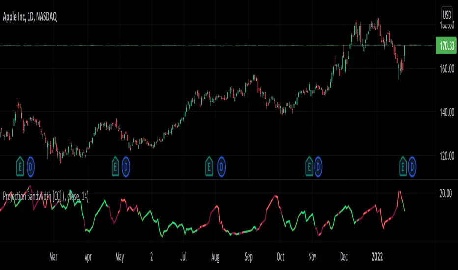
Projection Bandwidth [CC]The Projection Bandwidth was created by Mel Widner (Stocks and Commodities Jul 1995) and this is another of my series of indicators that I consider undiscovered gems. For those of you who are unaware, the Bandwidth indicator measures the distance between the high and low bands and if you remember from my Projection Bands script, the Projection Bands give pretty accurate early signals of trend reversals and followed fairly closely by a large bulge in the bands. The large bulges in the bands essentially act as the confirmation that the trend reversal is happening and so that brings me to this indicator. This indicator gives signals based on if it has reached a peak or a valley. Both extremes mean that the current trend is ending and I have color coded it based on the buy and sell signals from my Projection Bands indicator. I have included strong buy and sell signals in addition to normal ones so strong signals are darker in color and normal signals are lighter in color. Buy when the line turns green and sell when it turns red.
Let me know if there are any other scripts or indicators you would like to see me publish!
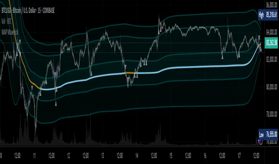
WAP Maverick - (Dual EMA Smoothed VWAP) - [mutantdog]Short Version:
This here is my take on the popular VWAP indicator with several novel features including:
Dual EMA smoothing.
Arithmetic and Harmonic Mean plots.
Custom Anchor feat. Intraday Session Sizes.
2 Pairs of Bands.
Side Input for Connection to other Indicator.
This can be used 'out of the box' as a replacement VWAP, benefitting from smoother transitions and easy-to-use custom alerts.
By design however, this is intended to be a highly customisable alternative with many adjustable parameters and a pseudo-modular input system to connect with another indicator. Well suited for the tweakers around here and those who like to get a little more creative.
I made this primarily for crypto although it should work for other markets. Default settings are best suited to 15m timeframe - the anchor of 1 week is ideal for crypto which often follows a cyclical nature from Monday through Sunday. In 15m, the default ema length of 21 means that the wap comes to match a standard vwap towards the end of Monday. If using higher chart timeframes, i recommend decreasing the ema length to closely match this principle (suggested: for 1h chart, try length = 8; for 4h chart, length = 2 or 3 should suffice).
Note: the use of harmonic mean calculations will cause problems on any data source incorporating both positive and negative values, it may also return unusable results on extremely low-value charts (eg: low-sat coins in /btc pairs).
Long version:
The development of this project was one driven more by experimentation than a specific end-goal, however i have tried to fine-tune everything into a coherent usable end-product. With that in mind then, this walkthrough will follow something of a development chronology as i dissect the various functions.
DUAL-EMA SMOOTHING
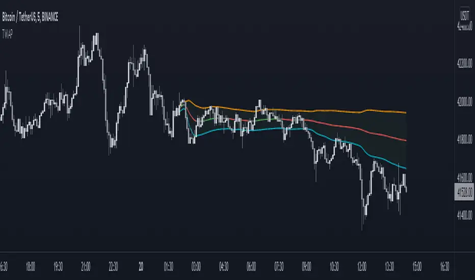
At its core this is based upon / adapted from the standard vwap indicator provided by TradingView although I have modified and changed most of it. The first mod is the dual ema smoothing. Rather than simply applying an ema to the output of the standard vwap function, instead i have incorporated the ema in a manner analogous to the way smas are used within a standard vwma. Sticking for now with the arithmetic mean, the basic vwap calculation is simply sum(source * volume) / sum(volume) across the anchored period. In this case i have simply applied an ema to each of the numerator and denominator values resulting in ema(sum(source * volume)) / ema(sum(volume)) with the ema length independent of the anchor. This results in smoother (albeit slower) transitions than the aforementioned post-vwap method. Furthermore in the case when anchor period is equal to current timeframe, the result is a basic volume-weighted ema.
The example below shows a standard vwap (1week anchor) in blue, a 21-ema applied to the vwap in purple and a dual-21-ema smoothed wap in gold. Notably both ema types come to effectively resemble the standard vwap after around 24 hours into the new anchor session but how they behave in the meantime is very different. The dual-ema transitions quite gradually while the post-vwap ema immediately sets about trying to catch up. Incidentally. a similar and slower variation of the dual-ema can be achieved with dual-rma although i have not included it in this indicator, attempted analogues using sma or wma were far less useful however.
STANDARD DEVIATION AND BANDS
With this updated calculation, a corresponding update to the standard deviation is also required. The vwap has its own anchored volume-weighted st.dev but this cannot be used in combination with the ema smoothing so instead it has been recalculated appropriately. There are two pairs of bands with separate multipliers (stepped to 0.1x) and in both cases high and low bands can be activated or deactivated individually. An example usage for this would be to create different upper and lower bands for profit and stoploss targets. Alerts can be set easily for different crossing conditions, more on this later.
Alongside the bands, i have also added the option to shift ('Deviate') the entire indicator up or down according to a multiple of the corrected st.dev value. This has many potential uses, for example if we want to bias our analysis in one direction it may be useful to move the wap in the opposite. Or if the asset is trading within a narrow range and we are waiting on a breakout, we could shift to the desired level and set alerts accordingly. The 'Deviate' parameter applies to the entire indicator including the bands which will remain centred on the main WAP.
CUSTOM (W)ANCHOR
Ever thought about using a vwap with anchor periods smaller than a day? Here you can do just that. I've removed the Earnings/Dividends/Splits options from the basic vwap and added an 'Intraday' option instead. When selected, a custom anchor length can be created as a multiple of minutes (default steps of 60 mins but can input any value from 0 - 1440). While this may not seem at first like a useful feature for anyone except hi-speed scalpers, this actually offers more interesting potential than it appears.
When set to 0 minutes the current timeframe is always used, turning this into the basic volume-weighted ema mentioned earlier. When using other low time frames the anchor can act as a pre-ema filter creating a stepped effect akin to an adaptive MA. Used in combination with the bands, the result is a kind of volume-weighted adaptive exponential bollinger band; if such a thing does not already exist then this is where you create it. Alternatively, by combining two instances you may find potential interesting crosses between an intraday wap and a standard timeframe wap. Below is an example set to intraday with 480 mins, 2x st.dev bands and ema length 21. Included for comparison in purple is a standard 21 ema.
I'm sure there are many potential uses to be found here, so be creative and please share anything you come up with in the comments.
ARITHMETIC AND HARMONIC MEAN CALCULATIONS
The standard vwap uses the arithmetic mean in its calculation. Indeed, most mean calculations tend to be arithmetic: sma being the most widely used example. When volume weighting is involved though this can lead to a slight bias in favour of upward moves over downward. While the effect of this is minor, over longer anchor periods it can become increasingly significant. The harmonic mean, on the other hand, has the opposite effect which results in a value that is always lower than the arithmetic mean. By viewing both arithmetic and harmonic waps together, the extent to which they diverge from each other can be used as a visual reference of how much price has changed during the anchored period.
Furthermore, the harmonic mean may actually be the more appropriate one to use during downtrends or bearish periods, in principle at least. Consider that a short trade is functionally the same as a long trade on the inverse of the pair (eg: selling BTC/USD is the same as buying USD/BTC). With the harmonic mean being an inverse of the arithmetic then, it makes sense to use it instead. To illustrate this below is a snapshot of LUNA/USDT on the left with its inverse 1/(LUNA/USDT) = USDT/LUNA on the right. On both charts is a wap with identical settings, note the resistance on the left and its corresponding support on the right. It should be easy from this to see that the lower harmonic wap on the left corresponds to the upper arithmetic wap on the right. Thus, it would appear that the harmonic mean should be used in a downtrend. In principle, at least...
In reality though, it is not quite so black and white. Rarely are these values exact in their predictions and the sort of range one should allow for inaccuracies will likely be greater than the difference between these two means. Furthermore, the ema smoothing has already introduced some lag and thus additional inaccuracies. Nevertheless, the symmetry warrants its inclusion.
SIDE INPUT & ALERTS
Finally we move on to the pseudo-modular component here. While TradingView allows some interoperability between indicators, it is limited to just one connection. Any attempt to use multiple source inputs will remove this functionality completely. The workaround here is to instead use custom 'string' input menus for additional sources, preserving this function in the sole 'source' input. In this case, since the wap itself is dependant only price and volume, i have repurposed the full 'source' into the second 'side' input. This allows for a separate indicator to interact with this one that can be used for triggering alerts. You could even use another instance of this one (there is a hidden wap:mid plot intended for this use which is the midpoint between both means). Note that deleting a connected indicator may result in the deletion of those connected to it.
Preset alertconditions are available for crossings of the side input above and below the main wap, alongside several customisable alerts with corresponding visual markers based upon selectable conditions. Alerts for band crossings apply only to those that are active and only crossings of the type specified within the 'crosses' subsection of the indicator settings. The included options make it easy to create buy alerts specific to certain bands with sell alerts specific to other bands. The chart below shows two instances with differing anchor periods, both are connected with buy and sell alerts enabled for visible bands.
Okay... So that just about covers it here, i think. As mentioned earlier this is the product of various experiments while i have been learning my way around PineScript. Some of those experiments have been branched off from this in order to not over-clutter it with functions. The pseudo-modular design and the 'side' input are the result of an attempt to create a connective framework across various projects. Even on its own though, this should offer plenty of tweaking potential for anyone who likes to venture away from the usual standards, all the while still retaining its core purpose as a traders tool.
Thanks for checking this out. I look forward to any feedback below.
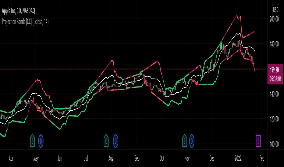
Projection Bands [CC]The Projection Bands were created by Mel Widner (Stocks and Commodities Jul 1995) and this indicator and the other two that rely on this one (I will publish them later) are very underappreciated in my humble opinion. The biggest strength of this indicator is the fact that it is a leading indicator for dramatic price movements. As you can see in my example chart it consistently gives great exit points before a downturn. I have included strong buy and sell signals in addition to normal ones so strong signals are darker in color and normal signals are lighter in color. Buy when the line turns green and sell when it turns red.
Let me know if there are any other indicators or scripts you would like to see me publish!
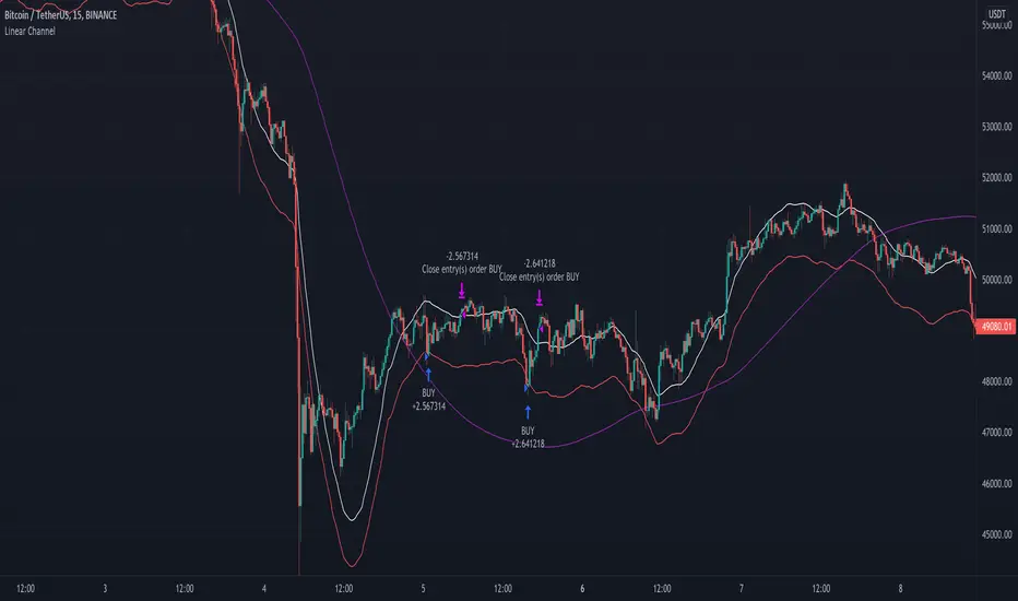
Linear Channel - Scalp Strategy 15MSimple way how to use Linear Regression for trading.
What we use:
• Linear Regression
• HMA as a trend filter
Logic:
Firstly we make simple linear regression moving. It is the white line which appears on the chart.
Then we make second line (named: band2) on the chart by multiplying linreg and value difference.
The third step is to ad HMA as a trend filter.
The trade open when price is below band2, but still upper than Hullma. The trade close when price again upper than linreg.

34 EMA Bands [v2]Updating an older concept here with some more oversold/overbought zones.
Pretty self explanatory, red zone indicate overbought zones and green zone is a oversold. Often, price likes to bounce off of the lower bounds of these zones, but it can sometimes extend all the way through the zone onto the upper boundary.
There are many lines to this indicator, i prefer using it with all the lines off except the outermost ones. However, you can edit it if it suits you better.
Source code is open, so any suggestions to improve its accuracy are welcome :)

34 EMA BandsThis is quite a simple script, just plotting a 34EMA on high's and low's of candles. Appears to work wonders though, so here it is.
There is some //'d code which I haven't finished working on, but it looks to be quite similar to Bollinger Bands, just using different math rather than standard deviations from the mean.
The bands itself is pretty self explanatory, price likes to use it as resistance when under it, it can trade inside it and it can use the upper EMA as support when in a strong upward trend.

Jurik Bands//A follow up for my JMA script. This script is inspired by (and dedicated to) closure of sales (today, Oct 20 '21) of the famous Jurik Research.
...
Jurik Research, the real people who been doing real things by using the real instruments, while many others been reading books "How to become a billionaire in 2 days", watching 5687 hours videos of how to use RSI , and studying+applying machine learning to everything cuz suddenly it became trendy xD
...
In my JMA script I've said that JMA takes into account volatility. But how exactly? In fact, it's based on smth called Jurik Bands. Thing is they can be/should be used as an independent instrument. I won't lie, I've developed smth very similar myself for mean-reverting purposes, but we ain't gonna talk about this now (my stuff is much simpler, saying bye-bye to entropy).
...
The code is on purpose in Pine4, because lmao I'm not gonna call my stuff "Indicators", they don't "Indicate" anything. And it's on purpose doesn't follow any "coding conventions" made by geeks to make their stuff look more important. My conventions are simple: less code as possible and as simple as possible so we can actually do business based on these instruments.
...
Live Long And Prosper