Price Statistical Strategy-Z Score V 1.01
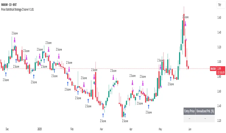
Price Statistical Strategy – Z Score V 1.01
Overview
A technical breakdown of the logic and components of the “Price Statistical Strategy – Z Score V 1.01”.
This script implements a smoothed Z-Score crossover mechanism applied to the closing price to detect potential statistical deviations from local price mean. The strategy operates solely on price data (close) and includes signal spacing control and momentum-based candle filters. No volume-based or trend-detection components are included.
Core Methodology
The strategy is built on the statistical concept of Z-Score, which quantifies how far a value (closing price) is from its recent average, normalized by standard deviation. Two moving averages of the raw Z-Score are calculated: a short-term and a long-term smoothed version. The crossover between them generates long entries and exits.
Signal Conditions
Entry Condition:
A long position is opened when the short-term smoothed Z-Score crosses above the long-term smoothed Z-Score, and additional entry conditions are met.
Exit Condition:
The position is closed when the short-term Z-Score crosses below the long-term Z-Score, provided the exit conditions allow.
Signal Gapping:
A minimum number of bars (Bars gap between identical signals) must pass between repeated entry or exit signals to reduce noise.
Momentum Filter:
Entries are prevented during sequences of three or more consecutively bullish candles, and exits are prevented during three or more consecutively bearish candles.
Z-Score Function
The Z-Score is calculated as:
Z = (Close - SMA(Close, N)) / STDEV(Close, N)
Where N is the base period selected by the user.
Input Parameters
Enable Smoothed Z-Score Strategy
Enables or disables the Z-Score strategy logic. When disabled, no trades are executed.
Z-Score Base Period
Defines the number of bars used to calculate the simple moving average and standard deviation for the Z-Score. This value affects how responsive the raw Z-Score is to price changes.
Short-Term Smoothing
Sets the smoothing window for the short-term Z-Score. Higher values produce smoother short-term signals, reducing sensitivity to short-term volatility.
Long-Term Smoothing
Sets the smoothing window for the long-term Z-Score, which acts as the reference line in the crossover logic.
Bars gap between identical signals
Minimum number of bars that must pass before another signal of the same type (entry or exit) is allowed. This helps reduce redundant or overly frequent signals.
Trade Visualization Table
A table positioned at the bottom-right displays live PnL for open trades:
Entry Price
Unrealized PnL %
Text colors adapt based on whether unrealized profit is positive, negative, or neutral.
Technical Notes
This strategy uses only close prices — no trend indicators or volume components are applied.
All calculations are based on simple moving averages and standard deviation over user-defined windows.
Designed as a minimal, isolated Z-Score engine without confirmation filters or multi-factor triggers.
Statistics
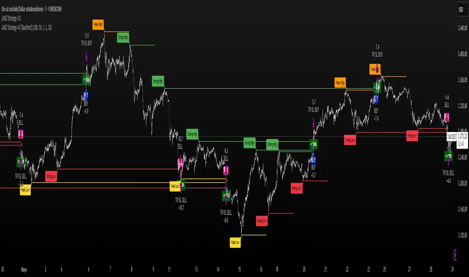
LANZ Strategy 4.0 [Backtest]🔷 LANZ Strategy 4.0 — Strategy Execution Based on Confirmed Structure + Risk-Based SL/TP
LANZ Strategy 4.0 is the official backtesting engine for the LANZ Strategy 4.0 trading logic. It simulates real-time executions based on breakout of Strong/Weak Highs or Lows, using a consistent structural system with SL/TP dynamically calculated per trade. With integrated risk management and lot size logic, this script allows traders to validate LANZ Strategy 4.0 performance with real strategy metrics.
🧠 Core Components:
Confirmed Breakout Entries: Trades are executed only when price breaks the most recent structural level (Strong High or Strong Low), detected using swing pivots.
Dynamic SL and TP Logic: SL is placed below/above the breakout point with a customizable buffer. TP is defined using a fixed Risk-Reward (RR) ratio.
Capital-Based Risk Management: Lot size is calculated based on account equity, SL distance, and pip value (e.g. $10 per pip on XAUUSD).
Clean and Controlled Executions: Only one trade is active at a time. No new entries are allowed until the current position is closed.
📊 Visual Features:
Automatic plotting of Entry, SL, and TP levels.
Full control of swing sensitivity (swingLength) and SL buffer.
SL and TP lines extend visually for clarity of trade risk and reward zones.
⚙️ How It Works:
Detects pivots and classifies trend direction.
Waits for breakout above Strong High (BUY) or below Strong Low (SELL).
Calculates dynamic SL and TP based on buffer and RR.
Computes trade size automatically based on risk per trade %.
Executes entry and manages exits via strategy engine.
📝 Notes:
Ideal for evaluating the LANZ Strategy 4.0 logic over historical data.
Must be paired with the original indicator (LANZ Strategy 4.0) for live trading.
Best used on assets with clear structural behavior (gold, indices, FX).
📌 Credits:
Backtest engine developed by LANZ based on the official rules of LANZ Strategy 4.0. This script ensures visual and logical consistency between live charting and backtesting simulations.
LANZ Strategy 3.0 [Backtest]🔷 LANZ Strategy 3.0 — Asian Range Fibonacci Scalping Strategy
LANZ Strategy 3.0 is a precision-engineered backtesting tool tailored for intraday traders who rely on the Asian session range to determine directional bias. This strategy implements dynamic Fibonacci projections and strict time-window validation to simulate a clean and disciplined trading environment.
🧠 Core Components:
Asian Range Bias Definition: Direction is established between 01:15–02:15 a.m. NY time based on the candle’s close in relation to the midpoint of the Asian session range (18:00–01:15 NY).
Limit Order Execution: Only one trade is placed daily, using a limit order at the Asian range high (for sells) or low (for buys), between 01:15–08:00 a.m. NY.
Fibonacci-Based TP/SL:
Original Mode: TP = 2.25x range, SL = 0.75x range.
Optimized Mode: TP = 1.95x range, SL = 0.65x range.
No Trade After 08:00 NY: If the limit order is not executed before 08:00 a.m. NY, it is canceled.
Fallback Logic at 02:15 NY: If the market direction misaligns with the setup at 02:15 a.m., the system re-evaluates and can re-issue the order.
End-of-Day Closure: All positions are closed at 15:45 NY if still open.
📊 Backtest-Ready Design:
Entries and exits are executed using strategy.entry() and strategy.exit() functions.
Position size is fixed via capital risk allocation ($100 per trade by default).
Only one position can be active at a time, ensuring controlled risk.
📝 Notes:
This strategy is ideal for assets sensitive to the Asian/London session overlap, such as Forex pairs and indices.
Easily switch between Fibonacci versions using a single dropdown input.
Fully deterministic: all entries are based on pre-defined conditions and time constraints.
👤 Credits:
Strategy developed by rau_u_lanz using Pine Script v6. Built for traders who favor clean sessions, directional clarity, and consistent execution using time-based logic and Fibonacci projections.

LANZ Strategy 2.0 [Backtest]🔷 LANZ Strategy 2.0 — Structural Breakout Logic with Dynamic Swing Protection
LANZ Strategy 2.0 is a precision-focused backtesting system built for intraday traders who rely on structural confirmations before the London session to guide directional bias. This tool uses smart swing detection, risk-defined position sizing, and strict time-based execution to simulate real trading conditions with clarity and control.
🧠 Core Components:
Structural Confirmation (Trend & BoS): Detects trend direction and break of structure (BoS) using a three-swing logic, aligning trade entries with valid structural movement.
Time-Based Execution: Trades are triggered exclusively at 02:00 a.m. New York time, ensuring disciplined and repeatable intraday testing.
Swing-Based SL Models: Traders can select between three stop-loss protection types:
First Swing: Most recent structural level
Second Swing: Prior level
Full Coverage: All recent swing levels + configurable pip buffer
Dynamic TP Calculation: Take-Profit is projected as a risk-based multiple (RR), fully adjustable via input.
Capital-Based Risk Management: Risk is defined as a percentage of a fixed account size (e.g., $100 per trade from $10,000), and lot size is automatically calculated based on SL distance.
Fallback Entry Logic: If structural breakout is present but trend is not confirmed, a secondary entry is triggered.
End-of-Session Management: Any open trades are automatically closed at 11:45 a.m. NY time, with optional manual labeling or review.
📊 Visual Features (Optional in Indicator Version):
(Note: Visuals apply to the indicator version of LANZ 2.0, not this backtest script)
Swing level labels (1st, 2nd) and dynamic SL/TP lines.
Real-time session coloring for clarity: Pre-London, Entry Window, and NY Close.
Outcome labels: +RR, -RR, or net % at close.
Auto-cleanup of previous drawings for a clean chart per session.
⚙️ How It Works:
Detects last trend and BoS using swing logic before 02:00 a.m. NY.
At 02:00 a.m., evaluates directional bias and executes BUY or SELL if confirmed.
Applies selected SL logic (1st, 2nd, or full swing protection).
Sets TP based on the RR multiplier.
Closes the trade either on SL, TP, or at 11:45 a.m. NY manually.
🔔 Alerts:
Time-of-day alert at 02:00 a.m. NY to monitor execution.
Can be extended to cover SL/TP triggers or new BoS events.
📝 Notes:
Designed for backtesting precision and discretionary decision-making.
Ideal for Forex pairs, indices, or assets active during the London session.
Fully customizable: session timing, swing logic, SL buffer, and RR.
👤 Credits:
Strategy built by @rau_u_lanz using Pine Script v6, combining structural logic, capital-based risk control, and London-session timing in a backtest-ready framework for traders who demand accuracy and structure.

Reverse Keltner Channel StrategyReverse Keltner Channel Strategy
Overview
The Reverse Keltner Channel Strategy is a mean-reversion trading system that capitalizes on price movements between Keltner Channels. Unlike traditional Keltner Channel strategies that trade breakouts, this system takes the contrarian approach by entering positions when price returns to the channel after overextending.
Strategy Logic
Long Entry Conditions:
Price crosses above the lower Keltner Channel from below
This signals a potential reversal after an oversold condition
Position is entered at market price upon signal confirmation
Long Exit Conditions:
Take Profit: Price reaches the upper Keltner Channel
Stop Loss: Placed at half the channel width below entry price
Short Entry Conditions:
Price crosses below the upper Keltner Channel from above
This signals a potential reversal after an overbought condition
Position is entered at market price upon signal confirmation
Short Exit Conditions:
Take Profit: Price reaches the lower Keltner Channel
Stop Loss: Placed at half the channel width above entry price
Key Features
Mean Reversion Approach: Takes advantage of price tendency to return to mean after extreme moves
Adaptive Stop Loss: Stop loss dynamically adjusts based on market volatility via ATR
Visual Signals: Entry points clearly marked with directional triangles
Fully Customizable: All parameters can be adjusted to fit various market conditions
Customizable Parameters
Keltner EMA Length: Controls the responsiveness of the channel (default: 20)
ATR Multiplier: Determines channel width/sensitivity (default: 2.0)
ATR Length: Affects volatility calculation period (default: 10)
Stop Loss Factor: Adjusts risk management aggressiveness (default: 0.5)
Best Used On
This strategy performs well on:
Currency pairs with defined ranging behavior
Commodities that show cyclical price movements
Higher timeframes (4H, Daily) for more reliable signals
Markets with moderate volatility
Risk Management
The built-in stop loss mechanism automatically adjusts to market conditions by calculating position risk relative to the current channel width. This approach ensures that risk remains proportional to potential reward across varying market conditions.
Notes for Optimization
Consider adjusting the EMA length and ATR multiplier based on the specific asset and timeframe:
Lower values increase sensitivity and generate more signals
Higher values produce fewer but potentially more reliable signals
As with any trading strategy, thorough backtesting is recommended before live implementation.
Past performance is not indicative of future results. Always practice sound risk management.

Daily Breakout + Daily Shadow By RouroThis script is a Pine v5 strategy designed to detect daily candle body breakouts and execute them on any intraday timeframe, while also providing:
Daily Data Retrieval
Using request.security(..., "D", ...) it fetches the OHLC and timestamp of the daily candle, regardless of the chart’s current timeframe.
Calculation of Yesterday’s and Day-Before-Yesterday’s Bodies
b1High and b1Low → the high/low of yesterday’s daily candle body
b2High and b2Low → the high/low of the previous day’s body
Detection of the First Intraday Bar After a New Day
By using ta.change(time("D")), it marks the start of each new trading day.
Drawing the Previous Day’s “Shadow” on the Chart
It overlays a box (box.new) and two wick lines (line.new) with configurable colors and transparency, so you can clearly see the full range of yesterday’s candle on any intraday chart.
Automatic End-of-Day Position Closure
It will automatically close any open position at the start of the next day to avoid unintended rollovers.
Entry Signals
On the very first intraday bar after the daily close:
Long if yesterday’s close broke above the body of the day before yesterday
Short if yesterday’s close broke below the body of the day before yesterday
…which triggers a strategy.entry at the intraday open.
Fully Customizable Stop-Loss and Take-Profit
SL options:
Opposite end of yesterday’s body
Fixed pips from entry
A risk-reward ratio on yesterday’s wick
Optional “safety SL” in fixed pips that overrides the above
TP options:
Fixed pips
Yesterday’s wick extreme (high/low)
Partial exit on the wick (TP1), then second exit (TP2) either:
At a multiplied RR
Or at the daily close (“Close of Day”)
You can also choose to move SL to breakeven after TP1 is hit.
Live Metrics Table
In the upper-right corner it displays in real time:
Start of backtest (date of first trade)
Number of ✅ Winning trades and ❌ Losing trades
Total number of trades
Win rate (%)
Profit Factor
All within a fixed table layout so it never runs out of rows or columns.

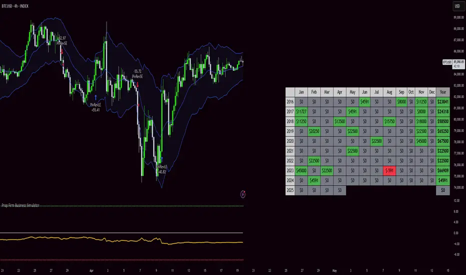
Prop Firm Business SimulatorThe prop firm business simulator is exactly what it sounds like. It's a plug and play tool to test out any tradingview strategy and simulate hypothetical performance on CFD Prop Firms.
Now what is a modern day CFD Prop Firm?
These companies sell simulated trading challenges for a challenge fee. If you complete the challenge you get access to simulated capital and you get a portion of the profits you make on those accounts payed out.
I've included some popular firms in the code as presets so it's easy to simulate them. Take into account that this info will likely be out of date soon as these prices and challenge conditions change.
Also, this tool will never be able to 100% simulate prop firm conditions and all their rules. All I aim to do with this tool is provide estimations.
Now why is this tool helpful?
Most traders on here want to turn their passion into their full-time career, prop firms have lately been the buzz in the trading community and market themselves as a faster way to reach that goal.
While this all sounds great on paper, it is sometimes hard to estimate how much money you will have to burn on challenge fees and set realistic monthly payout expectations for yourself and your trading. This is where this tool comes in.
I've specifically developed this for traders that want to treat prop firms as a business. And as a business you want to know your monthly costs and income depending on the trading strategy and prop firm challenge you are using.
How to use this tool
It's quite simple you remove the top part of the script and replace it with your own strategy. Make sure it's written in same version of pinescript before you do that.
//--$$$$$$$$$$$$$$$$$$$$$$$$$$$$$$$$$$$$$$$$$$$$$$$$--//--------------------------------------------------------------------------------------------------------------------------$$$$$$
//--$$$$$--Strategy-- --$$$$$$--// ******************************************************************************************************************************
//--$$$$$$$$$$$$$$$$$$$$$$$$$$$$$$$$$$$$$$$$$$$$$$$$--//--------------------------------------------------------------------------------------------------------------------------$$$$$$
length = input.int(20, minval=1, group="Keltner Channel Breakout")
mult = input(2.0, "Multiplier", group="Keltner Channel Breakout")
src = input(close, title="Source", group="Keltner Channel Breakout")
exp = input(true, "Use Exponential MA", display = display.data_window, group="Keltner Channel Breakout")
BandsStyle = input.string("Average True Range", options = , title="Bands Style", display = display.data_window, group="Keltner Channel Breakout")
atrlength = input(10, "ATR Length", display = display.data_window, group="Keltner Channel Breakout")
esma(source, length)=>
s = ta.sma(source, length)
e = ta.ema(source, length)
exp ? e : s
ma = esma(src, length)
rangema = BandsStyle == "True Range" ? ta.tr(true) : BandsStyle == "Average True Range" ? ta.atr(atrlength) : ta.rma(high - low, length)
upper = ma + rangema * mult
lower = ma - rangema * mult
//--Graphical Display--// *-*-*-*-*-*-*-*-*-*-*-*-*-*-*-*-*-*-*-*-*-*-*-*-*-*-*-*-*-*-*-*-*-*-*-*-*-*-*-*-*-*-*-*-*-*-*-*-*-*-*-*-*-*-*-*-*-*-*-*-*-*-*-*-*-*-*-*-*-*-*-*-*-$$$$$$
u = plot(upper, color=#2962FF, title="Upper", force_overlay=true)
plot(ma, color=#2962FF, title="Basis", force_overlay=true)
l = plot(lower, color=#2962FF, title="Lower", force_overlay=true)
fill(u, l, color=color.rgb(33, 150, 243, 95), title="Background")
//--Risk Management--// *-*-*-*-*-*-*-*-*-*-*-*-*-*-*-*-*-*-*-*-*-*-*-*-*-*-*-*-*-*-*-*-*-*-*-*-*-*-*-*-*-*-*-*-*-*-*-*-*-*-*-*-*-*-*-*-*-*-*-*-*-*-*-*-*-*-*-*-*-*-*-*-*-*-$$$$$$
riskPerTradePerc = input.float(1, title="Risk per trade (%)", group="Keltner Channel Breakout")
le = high>upper ? false : true
se = lowlower
strategy.entry('PivRevLE', strategy.long, comment = 'PivRevLE', stop = upper, qty=riskToLots)
if se and upper>lower
strategy.entry('PivRevSE', strategy.short, comment = 'PivRevSE', stop = lower, qty=riskToLots)
The tool will then use the strategy equity of your own strategy and use this to simulat prop firms. Since these CFD prop firms work with different phases and payouts the indicator will simulate the gains until target or max drawdown / daily drawdown limit gets reached. If it reaches target it will go to the next phase and keep on doing that until it fails a challenge.
If in one of the phases there is a reward for completing, like a payout, refund, extra it will add this to the gains.
If you fail the challenge by reaching max drawdown or daily drawdown limit it will substract the challenge fee from the gains.
These gains are then visualised in the calendar so you can get an idea of yearly / monthly gains of the backtest. Remember, it is just a backtest so no guarantees of future income.
The bottom pane (non-overlay) is visualising the performance of the backtest during the phases. This way u can check if it is realistic. For instance if it only takes 1 bar on chart to reach target you are probably risking more than the firm wants you to risk. Also, it becomes much less clear if daily drawdown got hit in those high risk strategies, the results will be less accurate.
The daily drawdown limit get's reset every time there is a new dayofweek on chart.
If you set your prop firm preset setting to "'custom" the settings below that are applied as your prop firm settings. Otherwise it will use one of the template by default it's FTMO 100K.
The strategy I'm using as an example in this script is a simple Keltner Channel breakout strategy. I'm using a 0.05% commission per trade as that is what I found most common on crypto exchanges and it's close to the commissions+spread you get on a cfd prop firm. I'm targeting a 1% risk per trade in the backtest to try and stay within prop firm boundaries of max 1% risk per trade.
Lastly, the original yearly and monthly performance table was developed by Quantnomad and I've build ontop of that code. Here's a link to the original publication:
That's everything for now, hope this indicator helps people visualise the potential of prop firms better or to understand that they are not a good fit for their current financial situation.
Strategy Stats [presentTrading]Hello! it's another weekend. This tool is a strategy performance analysis tool. Looking at the TradingView community, it seems few creators focus on this aspect. I've intentionally created a shared version. Welcome to share your idea or question on this.
█ Introduction and How it is Different
Strategy Stats is a comprehensive performance analytics framework designed specifically for trading strategies. Unlike standard strategy backtesting tools that simply show cumulative profits, this analytics suite provides real-time, multi-timeframe statistical analysis of your trading performance.
Multi-timeframe analysis: Automatically tracks performance metrics across the most recent time periods (last 7 days, 30 days, 90 days, 1 year, and 4 years)
Advanced statistical measures: Goes beyond basic metrics to include Information Coefficient (IC) and Sortino Ratio
Real-time feedback: Updates performance statistics with each new trade
Visual analytics: Color-coded performance table provides instant visual feedback on strategy health
Integrated risk management: Implements sophisticated take profit mechanisms with 3-step ATR and percentage-based exits
BTCUSD Performance
The table in the upper right corner is a comprehensive performance dashboard showing trading strategy statistics.
Note: While this presentation uses Vegas SuperTrend as the underlying strategy, this is merely an example. The Stats framework can be applied to any trading strategy. The Vegas SuperTrend implementation is included solely to demonstrate how the analytics module integrates with a trading strategy.
⚠️ Timeframe Limitations
Important: TradingView's backtesting engine has a maximum storage limit of 10,000 bars. When using this strategy stats framework on smaller timeframes such as 1-hour or 2-hour charts, you may encounter errors if your backtesting period is too long.
Recommended Timeframe Usage:
Ideal for: 4H, 6H, 8H, Daily charts and above
May cause errors on: 1H, 2H charts spanning multiple years
Not recommended for: Timeframes below 1H with long history
█ Strategy, How it Works: Detailed Explanation
The Strategy Stats framework consists of three primary components: statistical data collection, performance analysis, and visualization.
🔶 Statistical Data Collection
The system maintains several critical data arrays:
equityHistory: Tracks equity curve over time
tradeHistory: Records profit/loss of each trade
predictionSignals: Stores trade direction signals (1 for long, -1 for short)
actualReturns: Records corresponding actual returns from each trade
For each closed trade, the system captures:
float tradePnL = strategy.closedtrades.profit(tradeIndex)
float tradeReturn = strategy.closedtrades.profit_percent(tradeIndex)
int tradeType = entryPrice < exitPrice ? 1 : -1 // Direction
🔶 Performance Metrics Calculation
The framework calculates several key performance metrics:
Information Coefficient (IC):
The correlation between prediction signals and actual returns, measuring forecast skill.
IC = Correlation(predictionSignals, actualReturns)
Where Correlation is the Pearson correlation coefficient:
Correlation(X,Y) = (nΣXY - ΣXY) / √
Sortino Ratio:
Measures risk-adjusted return focusing only on downside risk:
Sortino = (Avg_Return - Risk_Free_Rate) / Downside_Deviation
Where Downside Deviation is:
Downside_Deviation = √
R_i represents individual returns, T is the target return (typically the risk-free rate), and n is the number of observations.
Maximum Drawdown:
Tracks the largest percentage drop from peak to trough:
DD = (Peak_Equity - Trough_Equity) / Peak_Equity * 100
🔶 Time Period Calculation
The system automatically determines the appropriate number of bars to analyze for each timeframe based on the current chart timeframe:
bars_7d = math.max(1, math.round(7 * barsPerDay))
bars_30d = math.max(1, math.round(30 * barsPerDay))
bars_90d = math.max(1, math.round(90 * barsPerDay))
bars_365d = math.max(1, math.round(365 * barsPerDay))
bars_4y = math.max(1, math.round(365 * 4 * barsPerDay))
Where barsPerDay is calculated based on the chart timeframe:
barsPerDay = timeframe.isintraday ?
24 * 60 / math.max(1, (timeframe.in_seconds() / 60)) :
timeframe.isdaily ? 1 :
timeframe.isweekly ? 1/7 :
timeframe.ismonthly ? 1/30 : 0.01
🔶 Visual Representation
The system presents performance data in a color-coded table with intuitive visual indicators:
Green: Excellent performance
Lime: Good performance
Gray: Neutral performance
Orange: Mediocre performance
Red: Poor performance
█ Trade Direction
The Strategy Stats framework supports three trading directions:
Long Only: Only takes long positions when entry conditions are met
Short Only: Only takes short positions when entry conditions are met
Both: Takes both long and short positions depending on market conditions
█ Usage
To effectively use the Strategy Stats framework:
Apply to existing strategies: Add the performance tracking code to any strategy to gain advanced analytics
Monitor multiple timeframes: Use the multi-timeframe analysis to identify performance trends
Evaluate strategy health: Review IC and Sortino ratios to assess predictive power and risk-adjusted returns
Optimize parameters: Use performance data to refine strategy parameters
Compare strategies: Apply the framework to multiple strategies to identify the most effective approach
For best results, allow the strategy to generate sufficient trade history for meaningful statistical analysis (at least 20-30 trades).
█ Default Settings
The default settings have been carefully calibrated for cryptocurrency markets:
Performance Tracking:
Time periods: 7D, 30D, 90D, 1Y, 4Y
Statistical measures: Return, Win%, MaxDD, IC, Sortino Ratio
IC color thresholds: >0.3 (green), >0.1 (lime), <-0.1 (orange), <-0.3 (red)
Sortino color thresholds: >1.0 (green), >0.5 (lime), <0 (red)
Multi-Step Take Profit:
ATR multipliers: 2.618, 5.0, 10.0
Percentage levels: 3%, 8%, 17%
Short multiplier: 1.5x (makes short take profits more aggressive)
Stop loss: 20%

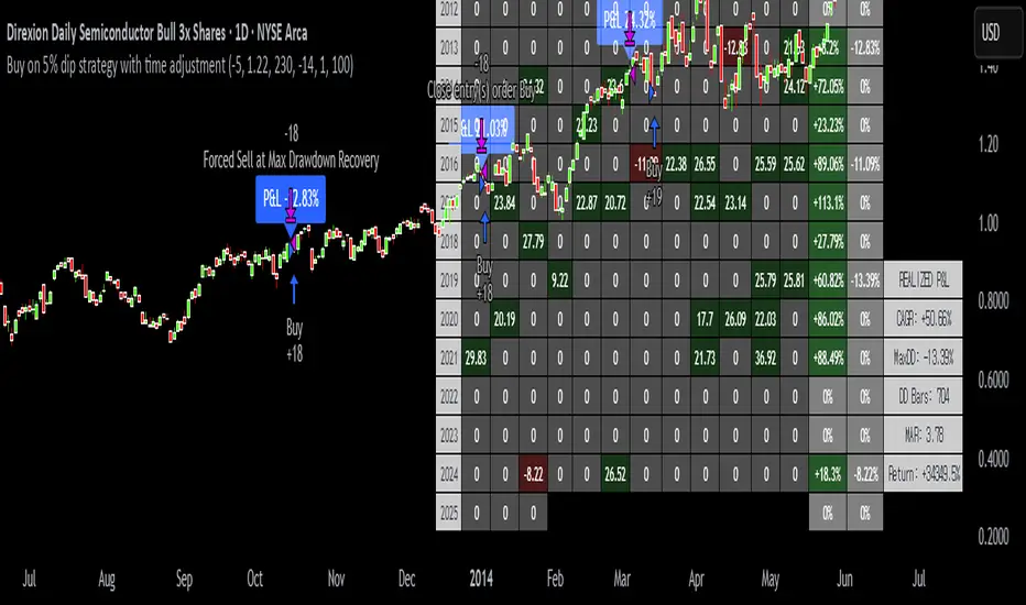
Buy on 5% dip strategy with time adjustment
This script is a strategy called "Buy on 5% Dip Strategy with Time Adjustment 📉💡," which detects a 5% drop in price and triggers a buy signal 🔔. It also automatically closes the position once the set profit target is reached 💰, and it has additional logic to close the position if the loss exceeds 14% after holding for 230 days ⏳.
Strategy Explanation
Buy Condition: A buy signal is triggered when the price drops 5% from the highest price reached 🔻.
Take Profit: The position is closed when the price hits a 1.22x target from the average entry price 📈.
Forced Sell Condition: If the position is held for more than 230 days and the loss exceeds 14%, the position is automatically closed 🚫.
Leverage & Capital Allocation: Leverage is adjustable ⚖️, and you can set the percentage of capital allocated to each trade 💸.
Time Limits: The strategy allows you to set a start and end time ⏰ for trading, making the strategy active only within that specific period.
Code Credits and References
Credits: This script utilizes ideas and code from @QuantNomad and jangdokang for the profit table and algorithm concepts 🔧.
Sources:
Monthly Performance Table Script by QuantNomad:
ZenAndTheArtOfTrading's Script:
Strategy Performance
This strategy provides risk management through take profit and forced sell conditions and includes a performance table 📊 to track monthly and yearly results. You can compare backtest results with real-time performance to evaluate the strategy's effectiveness.
The performance numbers shown in the backtest reflect what would have happened if you had used this strategy since the launch date of the SOXL (the Direxion Daily Semiconductor Bull 3x Shares ETF) 📅. These results are not hypothetical but based on actual performance from the day of the ETF’s launch 📈.
Caution ⚠️
No Guarantee of Future Results: The results are based on historical performance from the launch of the SOXL ETF, but past performance does not guarantee future results. It’s important to approach with caution when applying it to live trading 🔍.
Risk Management: Leverage and capital allocation settings are crucial for managing risk ⚠️. Make sure to adjust these according to your risk tolerance ⚖️.
Simple APF Strategy Backtesting [The Quant Science]Simple backtesting strategy for the quantitative indicator Autocorrelation Price Forecasting. This is a Buy & Sell strategy that operates exclusively with long orders. It opens long positions and generates profit based on the future price forecast provided by the indicator. It's particularly suitable for trend-following trading strategies or directional markets with an established trend.
Main functions
1. Cycle Detection: Utilize autocorrelation to identify repetitive market behaviors and cycles.
2. Forecasting for Backtesting: Simulate trades and assess the profitability of various strategies based on future price predictions.
Logic
The strategy works as follow:
Entry Condition: Go long if the hypothetical gain exceeds the threshold gain (configurable by user interface).
Position Management: Sets a take-profit level based on the future price.
Position Sizing: Automatically calculates the order size as a percentage of the equity.
No Stop-Loss: this strategy doesn't includes any stop loss.
Example Use Case
A trader analyzes a dayli period using 7 historical bars for autocorrelation.
Sets a threshold gain of 20 points using a 5% of the equity for each trade.
Evaluates the effectiveness of a long-only strategy in this period to assess its profitability and risk-adjusted performance.
User Interface
Length: Set the length of the data used in the autocorrelation price forecasting model.
Thresold Gain: Minimum value to be considered for opening trades based on future price forecast.
Order Size: percentage size of the equity used for each single trade.
Strategy Limit
This strategy does not use a stop loss. If the price continues to drop and the future price forecast is incorrect, the trader may incur a loss or have their capital locked in the losing trade.
Disclaimer!
This is a simple template. Use the code as a starting point rather than a finished solution. The script does not include important parameters, so use it solely for educational purposes or as a boilerplate.

Fibonacci-Only Strategy V2Fibonacci-Only Strategy V2
This strategy combines Fibonacci retracement levels with pattern recognition and statistical confirmation to identify high-probability trading opportunities across multiple timeframes.
Core Strategy Components:
Fibonacci Levels: Uses key Fibonacci retracement levels (19% and 82.56%) to identify potential reversal zones
Pattern Recognition: Analyzes recent price patterns to find similar historical formations
Statistical Confirmation: Incorporates statistical analysis to validate entry signals
Risk Management: Includes customizable stop loss (fixed or ATR-based) and trailing stop features
Entry Signals:
Long entries occur when price touches or breaks the 19% Fibonacci level with bullish confirmation
Short entries require Fibonacci level interaction, bearish confirmation, and statistical validation
All signals are visually displayed with color-coded markers and dashboard
Trading Method:
When a triangle signal appears, open a position on the next candle
Alternatively, after seeing a signal on a higher timeframe, you can switch to a lower timeframe to find a more precise entry point
Entry signals are clearly marked with visual indicators for easy identification
Risk Management Features:
Adjustable stop loss (percentage-based or ATR-based)
Optional trailing stops for protecting profits
Multiple take-profit levels for strategic position exit
Customization Options:
Timeframe selection (1m to Daily)
Pattern length and similarity threshold adjustment
Statistical period and weight configuration
Risk parameters including stop loss and trailing stop settings
This strategy is particularly well-suited for cryptocurrency markets due to their tendency to respect Fibonacci levels and technical patterns. Crypto's volatility is effectively managed through the customizable stop-loss and trailing-stop mechanisms, making it an ideal tool for traders in digital asset markets.
For optimal performance, this strategy works best on higher timeframes (30m, 1h and above) and is not recommended for low timeframe scalping. The Fibonacci pattern recognition requires sufficient price movement to generate reliable signals, which is more consistently available in medium to higher timeframes.
Users should avoid trading during sideways market conditions, as the strategy performs best during trending markets with clear directional movement. The statistical confirmation component helps filter out some sideways market signals, but it's recommended to manually avoid ranging markets for best results.

Divergence IQ [TradingIQ]Hello Traders!
Introducing "Divergence IQ"
Divergence IQ lets traders identify divergences between price action and almost ANY TradingView technical indicator. This tool is designed to help you spot potential trend reversals and continuation patterns with a range of configurable features.
Features
Divergence Detection
Detects both regular and hidden divergences for bullish and bearish setups by comparing price movements with changes in the indicator.
Offers two detection methods: one based on classic pivot point analysis and another that provides immediate divergence signals.
Option to use closing prices for divergence detection, allowing you to choose the data that best fits your strategy.
Normalization Options:
Includes multiple normalization techniques such as robust scaling, rolling Z-score, rolling min-max, or no normalization at all.
Adjustable normalization window lets you customize the indicator to suit various market conditions.
Option to display the normalized indicator on the chart for clearer visual comparison.
Allows traders to take indicators that aren't oscillators, and convert them into an oscillator - allowing for better divergence detection.
Simulated Trade Management:
Integrates simulated trade entries and exits based on divergence signals to demonstrate potential trading outcomes.
Customizable exit strategies with options for ATR-based or percentage-based stop loss and profit target settings.
Automatically calculates key trade metrics such as profit percentage, win rate, profit factor, and total trade count.
Visual Enhancements and On-Chart Displays:
Color-coded signals differentiate between bullish, bearish, hidden bullish, and hidden bearish divergence setups.
On-chart labels, lines, and gradient flow visualizations clearly mark divergence signals, entry points, and exit levels.
Configurable settings let you choose whether to display divergence signals on the price chart or in a separate pane.
Performance Metrics Table:
A performance table dynamically displays important statistics like profit, win rate, profit factor, and number of trades.
This feature offers an at-a-glance assessment of how the divergence-based strategy is performing.
The image above shows Divergence IQ successfully identifying and trading a bullish divergence between an indicator and price action!
The image above shows Divergence IQ successfully identifying and trading a bearish divergence between an indicator and price action!
The image above shows Divergence IQ successfully identifying and trading a hidden bullish divergence between an indicator and price action!
The image above shows Divergence IQ successfully identifying and trading a hidden bearish divergence between an indicator and price action!
The performance table is designed to provide a clear summary of simulated trade results based on divergence setups. You can easily review key metrics to assess the strategy’s effectiveness over different time periods.
Customization and Adaptability
Divergence IQ offers a wide range of configurable settings to tailor the indicator to your personal trading approach. You can adjust the lookback and lookahead periods for pivot detection, select your preferred method for normalization, and modify trade exit parameters to manage risk according to your strategy. The tool’s clear visual elements and comprehensive performance metrics make it a useful addition to your technical analysis toolbox.
The image above shows Divergence IQ identifying divergences between price action and OBV with no normalization technique applied.
While traders can look for divergences between OBV and price, OBV doesn't naturally behave like an oscillator, with no definable upper and lower threshold, OBV can infinitely increase or decrease.
With Divergence IQ's ability to normalize any indicator, traders can normalize non-oscillator technical indicators such as OBV, CVD, MACD, or even a moving average.
In the image above, the "Robust Scaling" normalization technique is selected. Consequently, the output of OBV has changed and is now behaving similar to an oscillator-like technical indicator. This makes spotting divergences between the indicator and price easier and more appropriate.
The three normalization techniques included will change the indicator's final output to be more compatible with divergence detection.
This feature can be used with almost any technical indicator.
Stop Type
Traders can select between ATR based profit targets and stop losses, or percentage based profit targets and stop losses.
The image above shows options for the feature.
Divergence Detection Method
A natural pitfall of divergence trading is that it generally takes several bars to "confirm" a divergence. This makes trading the divergence complicated, because the entry at time of the divergence might look great; however, the divergence wasn't actually signaled until several bars later.
To circumvent this issue, Divergence IQ offers two divergence detection mechanisms.
Pivot Detection
Pivot detection mode is the same as almost every divergence indicator on TradingView. The Pivots High Low indicator is used to detect market/indicator highs and lows and, consequently, divergences.
This method generally finds the "best looking" divergences, but will always take additional time to confirm the divergence.
Immediate Detection
Immediate detection mode attempts to reduce lag between the divergence and its confirmation to as little as possible while avoiding repainting.
Immediate detection mode still uses the Pivots Detection model to find the first high/low of a divergence. However, the most recent high/low does not utilize the Pivot Detection model, and instead immediately looks for a divergence between price and an indicator.
Immediate Detection Mode will always signal a divergence one bar after it's occurred, and traders can set alerts in this mode to be alerted as soon as the divergence occurs.
TradingView Backtester Integration
Divergence IQ is fully compatible with the TradingView backtester!
Divergence IQ isn’t designed to be a “profitable strategy” for users to trade. Instead, the intention of including the backtester is to let users backtest divergence-based trading strategies between the asset on their chart and almost any technical indicator, and to see if divergences have any predictive utility in that market.
So while the backtester is available in Divergence IQ, it’s for users to personally figure out if they should consider a divergence an actionable insight, and not a solicitation that Divergence IQ is a profitable trading strategy. Divergence IQ should be thought of as a Divergence backtesting toolkit, not a full-feature trading strategy.
Strategy Properties Used For Backtest
Initial Capital: $1000 - a realistic amount of starting capital that will resonate with many traders
Amount Per Trade: 5% of equity - a realistic amount of capital to invest relative to portfolio size
Commission: 0.02% - a conservative amount of commission to pay for trade that is standard in crypto trading, and very high for other markets.
Slippage: 1 tick - appropriate for liquid markets, but must be increased in markets with low activity.
Once more, the backtester is meant for traders to personally figure out if divergences are actionable trading signals on the market they wish to trade with the indicator they wish to use.
And that's all!
If you have any cool features you think can benefit Divergence IQ - please feel free to share them!
Thank you so much TradingView community!

Iron Bot Statistical Trend Filter📌 Iron Bot Statistical Trend Filter
📌 Overview
Iron Bot Statistical Trend Filter is an advanced trend filtering strategy that combines statistical methods with technical analysis.
By leveraging Z-score and Fibonacci levels, this strategy quantitatively analyzes market trends to provide high-precision entry signals.
Additionally, it includes an optional EMA filter to enhance trend reliability.
Risk management is reinforced with Stop Loss (SL) and four Take Profit (TP) levels, ensuring a balanced approach to risk and reward.
📌 Key Features
🔹 1. Statistical Trend Filtering with Z-Score
This strategy calculates the Z-score to measure how much the price deviates from its historical mean.
Positive Z-score: Indicates a statistically high price, suggesting a strong uptrend.
Negative Z-score: Indicates a statistically low price, signaling a potential downtrend.
Z-score near zero: Suggests a ranging market with no strong trend.
By using the Z-score as a filter, market noise is reduced, leading to more reliable entry signals.
🔹 2. Fibonacci Levels for Trend Reversal Detection
The strategy integrates Fibonacci retracement levels to identify potential reversal points in the market.
High Trend Level (Fibo 23.6%): When the price surpasses this level, an uptrend is likely.
Low Trend Level (Fibo 78.6%): When the price falls below this level, a downtrend is expected.
Trend Line (Fibo 50%): Acts as a midpoint, helping to assess market balance.
This allows traders to visually confirm trend strength and turning points, improving entry accuracy.
🔹 3. EMA Filter for Trend Confirmation (Optional)
The strategy includes an optional 200 EMA (Exponential Moving Average) filter for trend validation.
Price above 200 EMA: Indicates a bullish trend (long entries preferred).
Price below 200 EMA: Indicates a bearish trend (short entries preferred).
Enabling this filter reduces false signals and improves trend-following accuracy.
🔹 4. Multi-Level Take Profit (TP) and Stop Loss (SL) Management
To ensure effective risk management, the strategy includes four Take Profit levels and a Stop Loss:
Stop Loss (SL): Automatically closes trades when the price moves against the position by a certain percentage.
TP1 (+0.75%): First profit-taking level.
TP2 (+1.1%): A higher probability profit target.
TP3 (+1.5%): Aiming for a stronger trend move.
TP4 (+2.0%): Maximum profit target.
This system secures profits at different stages and optimizes risk-reward balance.
🔹 5. Automated Long & Short Trading Logic
The strategy is built using Pine Script®’s strategy.entry() and strategy.exit(), allowing fully automated trading.
Long Entry:
Price is above the trend line & high trend level.
Z-score is positive (indicating an uptrend).
(Optional) Price is also above the EMA for stronger confirmation.
Short Entry:
Price is below the trend line & low trend level.
Z-score is negative (indicating a downtrend).
(Optional) Price is also below the EMA for stronger confirmation.
This logic helps filter out unnecessary trades and focus only on high-probability entries.
📌 Trading Parameters
This strategy is designed for flexible capital management and risk control.
💰 Account Size: $5000
📉 Commissions and Slippage: Assumes 94 pips commission per trade and 1 pip slippage.
⚖️ Risk per Trade: Adjustable, with a default setting of 1% of equity.
These parameters help preserve capital while optimizing the risk-reward balance.
📌 Visual Aids for Clarity
To enhance usability, the strategy includes clear visual elements for easy market analysis.
✅ Trend Line (Blue): Indicates market midpoint and helps with entry decisions.
✅ Fibonacci Levels (Yellow): Highlights high and low trend levels.
✅ EMA Line (Green, Optional): Confirms long-term trend direction.
✅ Entry Signals (Green for Long, Red for Short): Clearly marked buy and sell signals.
These features allow traders to quickly interpret market conditions, even without advanced technical analysis skills.
📌 Originality & Enhancements
This strategy is developed based on the IronXtreme and BigBeluga indicators,
combining a unique Z-score statistical method with Fibonacci trend analysis.
Compared to conventional trend-following strategies, it leverages statistical techniques
to provide higher-precision entry signals, reducing false trades and improving overall reliability.
📌 Summary
Iron Bot Statistical Trend Filter is a statistically-driven trend strategy that utilizes Z-score and Fibonacci levels.
High-precision trend analysis
Enhanced accuracy with an optional EMA filter
Optimized risk management with multiple TP & SL levels
Visually intuitive chart design
Fully customizable parameters & leverage support
This strategy reduces false signals and helps traders ride the trend with confidence.
Try it out and take your trading to the next level! 🚀

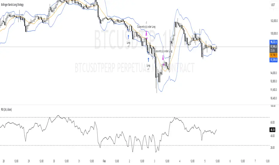
Bollinger Bands Long Strategy
This strategy is designed for identifying and executing long trades based on Bollinger Bands and RSI. It aims to capitalize on potential oversold conditions and subsequent price recovery.
Key Features:
- Bollinger Bands (10,2): The strategy uses Bollinger Bands with a 10-period moving average and a multiplier of 2 to define price volatility.
- RSI Filter: A trade is only triggered when the RSI (14-period) is below 30, ensuring entry during oversold conditions.
- Entry Condition: A long trade is entered immediately when the price crosses below the lower Bollinger Band and the RSI is under 30.
- Exit Condition: The position is exited when the price reaches or crosses above the Bollinger Band basis (20-period moving average).
Best Used For:
- Identifying oversold conditions with a strong potential for a rebound.
- Markets or assets with clear oscillations and volatility e.g., BTC.
**Disclaimer:** This strategy is for educational purposes and should be used with caution. Backtesting and risk management are essential before live trading.
Statistical Arbitrage Pairs Trading - Long-Side OnlyThis strategy implements a simplified statistical arbitrage (" stat arb ") approach focused on mean reversion between two correlated instruments. It identifies opportunities where the spread between their normalized price series (Z-scores) deviates significantly from historical norms, then executes long-only trades anticipating reversion to the mean.
Key Mechanics:
1. Spread Calculation: The strategy computes Z-scores for both instruments to normalize price movements, then tracks the spread between these Z-scores.
2. Modified Z-Score: Uses a robust measure combining the median and Median Absolute Deviation (MAD) to reduce outlier sensitivity.
3. Entry Signal: A long position is triggered when the spread’s modified Z-score falls below a user-defined threshold (e.g., -1.0), indicating extreme undervaluation of the main instrument relative to its pair.
4. Exit Signal: The position closes automatically when the spread reverts to its historical mean (Z-score ≥ 0).
Risk management:
Trades are sized as a percentage of equity (default: 10%).
Includes commissions and slippage for realistic backtesting.
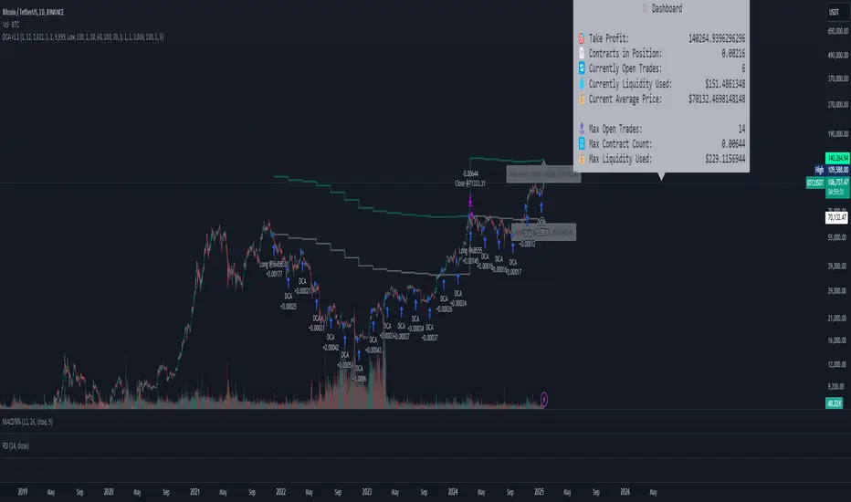
DCA Simulation for CryptoCommunity v1.1Overview
This script provides a detailed simulation of a Dollar-Cost Averaging (DCA) strategy tailored for crypto traders. It allows users to visualize how their DCA strategy would perform historically under specific parameters. The script is designed to help traders understand the mechanics of DCA and how it influences average price movement, budget utilization, and trade outcomes.
Key Features:
Combines Interval and Safety Order DCA:
Interval DCA: Regular purchases based on predefined time intervals.
Safety Order DCA: Additional buys triggered by percentage price drops.
Interactive Visualization:
Displays buy levels, average price, and profit-taking points on the chart.
Allows traders to assess how their strategy adapts to price movements.
Comprehensive Dashboard:
Tracks money spent, contracts acquired, and budget utilization.
Shows maximum amounts used if profit-taking is active.
Dynamic Safety Orders:
Resets safety orders when a new higher high is established.
Customizable Parameters:
Adjustable buy frequency, safety order settings, and profit-taking levels.
Suitable for traders with varying budgets and risk tolerances.
Default Strategy Settings:
Account Size: Default account size is set to $10,000 to represent a realistic budget for the average trader.
Commission & Slippage: Includes realistic trading fees and slippage assumptions to ensure accurate backtesting results.
Risk Management: Defaults to risking no more than 5% of the account balance per trade.
Sample Size: Optimized to generate a minimum of 100 trades for meaningful statistical analysis. Users can adjust parameters to fit longer timeframes or different datasets.
Usage Instructions:
Configure Your Strategy: Set the base order, safety order size, and buy frequency based on your preferred DCA approach.
Analyze Historical Performance: Use the chart and dashboard to understand how the strategy performs under different market conditions.
Optimize Parameters: Adjust settings to align with your risk tolerance and trading objectives.
Important Notes:
This script is for educational and simulation purposes. It is not intended to provide financial advice or guarantee profitability.
If the strategy's default settings do not meet your needs, feel free to adjust them while keeping risk management in mind.
TradingView limits the number of open trades to 999, so reduce the buy frequency if necessary to fit longer timeframes.
Mean Reversion Pro Strategy [tradeviZion]Mean Reversion Pro Strategy : User Guide
A mean reversion trading strategy for daily timeframe trading.
Introduction
Mean Reversion Pro Strategy is a technical trading system that operates on the daily timeframe. The strategy uses a dual Simple Moving Average (SMA) system combined with price range analysis to identify potential trading opportunities. It can be used on major indices and other markets with sufficient liquidity.
The strategy includes:
Trading System
Fast SMA for entry/exit points (5, 10, 15, 20 periods)
Slow SMA for trend reference (100, 200 periods)
Price range analysis (20% threshold)
Position management rules
Visual Elements
Gradient color indicators
Three themes (Dark/Light/Custom)
ATR-based visuals
Signal zones
Status Table
Current position information
Basic performance metrics
Strategy parameters
Optional messages
📊 Strategy Settings
Main Settings
Trading Mode
Options: Long Only, Short Only, Both
Default: Long Only
Position Size: 10% of equity
Starting Capital: $20,000
Moving Averages
Fast SMA: 5, 10, 15, or 20 periods
Slow SMA: 100 or 200 periods
Default: Fast=5, Slow=100
🎯 Entry and Exit Rules
Long Entry Conditions
All conditions must be met:
Price below Fast SMA
Price below 20% of current bar's range
Price above Slow SMA
No existing position
Short Entry Conditions
All conditions must be met:
Price above Fast SMA
Price above 80% of current bar's range
Price below Slow SMA
No existing position
Exit Rules
Long Positions
Exit when price crosses above Fast SMA
No fixed take-profit levels
No stop-loss (mean reversion approach)
Short Positions
Exit when price crosses below Fast SMA
No fixed take-profit levels
No stop-loss (mean reversion approach)
💼 Risk Management
Position Sizing
Default: 10% of equity per trade
Initial capital: $20,000
Commission: 0.01%
Slippage: 2 points
Maximum one position at a time
Risk Control
Use daily timeframe only
Avoid trading during major news events
Consider market conditions
Monitor overall exposure
📊 Performance Dashboard
The strategy includes a comprehensive status table displaying:
Strategy Parameters
Current SMA settings
Trading direction
Fast/Slow SMA ratio
Current Status
Active position (Flat/Long/Short)
Current price with color coding
Position status indicators
Performance Metrics
Net Profit (USD and %)
Win Rate with color grading
Profit Factor with thresholds
Maximum Drawdown percentage
Average Trade value
📱 Alert Settings
Entry Alerts
Long Entry (Buy Signal)
Short Entry (Sell Signal)
Exit Alerts
Long Exit (Take Profit)
Short Exit (Take Profit)
Alert Message Format
Strategy name
Signal type and direction
Current price
Fast SMA value
Slow SMA value
💡 Usage Tips
Consider starting with Long Only mode
Begin with default settings
Keep track of your trades
Review results regularly
Adjust settings as needed
Follow your trading plan
⚠️ Disclaimer
This strategy is for educational and informational purposes only. It is not financial advice. Always:
Conduct your own research
Test thoroughly before live trading
Use proper risk management
Consider your trading goals
Monitor market conditions
Never risk more than you can afford to lose
📋 Release Notes
14 January 2025
Added New Fast & Slow SMA Options:
Fibonacci-based periods: 8, 13, 21, 144, 233, 377
Additional period: 50
Complete Fast SMA options now: 5, 8, 10, 13, 15, 20, 21, 34, 50
Complete Slow SMA options now: 100, 144, 200, 233, 377
Bug Fixes:
Fixed Maximum Drawdown calculation in the performance table
Now using strategy.max_drawdown_percent for accurate DD reporting
Previous version showed incorrect DD values
Performance metrics now accurately reflect trading results
Performance Note:
Strategy tested with Fast/Slow SMA 13/377
Test conducted with 10% equity risk allocation
Daily Timeframe
For Beginners - How to Modify SMA Levels:
Find this line in the code:
fastLength = input.int(title="Fast SMA Length", defval=5, options= )
To add a new Fast SMA period: Add the number to the options list, e.g.,
To remove a Fast SMA period: Remove the number from the options list
For Slow SMA, find:
slowLength = input.int(title="Slow SMA Length", defval=100, options= )
Modify the options list the same way
⚠️ Note: Keep the periods that make sense for your trading timeframe
💡 Tip: Test any new combinations thoroughly before live trading
"Trade with Discipline, Manage Risk, Stay Consistent" - tradeviZion

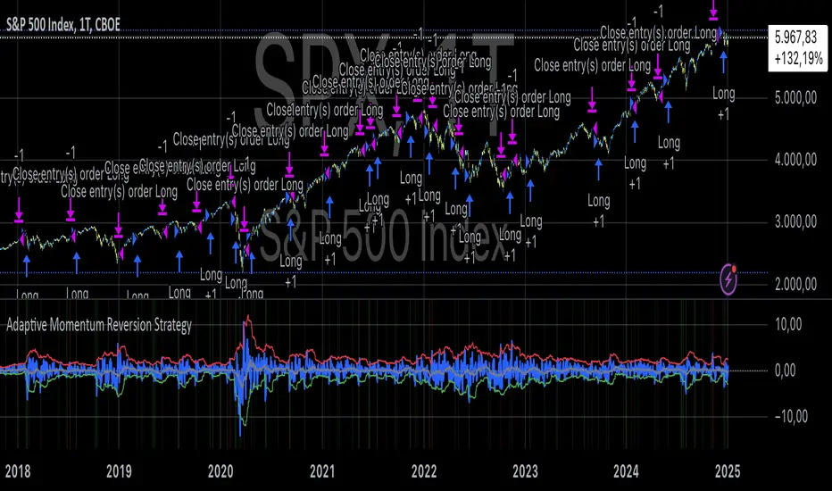
Adaptive Momentum Reversion StrategyThe Adaptive Momentum Reversion Strategy: An Empirical Approach to Market Behavior
The Adaptive Momentum Reversion Strategy seeks to capitalize on market price dynamics by combining concepts from momentum and mean reversion theories. This hybrid approach leverages a Rate of Change (ROC) indicator along with Bollinger Bands to identify overbought and oversold conditions, triggering trades based on the crossing of specific thresholds. The strategy aims to detect momentum shifts and exploit price reversions to their mean.
Theoretical Framework
Momentum and Mean Reversion: Momentum trading assumes that assets with a recent history of strong performance will continue in that direction, while mean reversion suggests that assets tend to return to their historical average over time (Fama & French, 1988; Poterba & Summers, 1988). This strategy incorporates elements of both, looking for periods when momentum is either overextended (and likely to revert) or when the asset’s price is temporarily underpriced relative to its historical trend.
Rate of Change (ROC): The ROC is a straightforward momentum indicator that measures the percentage change in price over a specified period (Wilder, 1978). The strategy calculates the ROC over a 2-period window, making it responsive to short-term price changes. By using ROC, the strategy aims to detect price acceleration and deceleration.
Bollinger Bands: Bollinger Bands are used to identify volatility and potential price extremes, often signaling overbought or oversold conditions. The bands consist of a moving average and two standard deviation bounds that adjust dynamically with price volatility (Bollinger, 2002).
The strategy employs two sets of Bollinger Bands: one for short-term volatility (lower band) and another for longer-term trends (upper band), with different lengths and standard deviation multipliers.
Strategy Construction
Indicator Inputs:
ROC Period: The rate of change is computed over a 2-period window, which provides sensitivity to short-term price fluctuations.
Bollinger Bands:
Lower Band: Calculated with a 18-period length and a standard deviation of 1.7.
Upper Band: Calculated with a 21-period length and a standard deviation of 2.1.
Calculations:
ROC Calculation: The ROC is computed by comparing the current close price to the close price from rocPeriod days ago, expressing it as a percentage.
Bollinger Bands: The strategy calculates both upper and lower Bollinger Bands around the ROC, using a simple moving average as the central basis. The lower Bollinger Band is used as a reference for identifying potential long entry points when the ROC crosses above it, while the upper Bollinger Band serves as a reference for exits, when the ROC crosses below it.
Trading Conditions:
Long Entry: A long position is initiated when the ROC crosses above the lower Bollinger Band, signaling a potential shift from a period of low momentum to an increase in price movement.
Exit Condition: A position is closed when the ROC crosses under the upper Bollinger Band, or when the ROC drops below the lower band again, indicating a reversal or weakening of momentum.
Visual Indicators:
ROC Plot: The ROC is plotted as a line to visualize the momentum direction.
Bollinger Bands: The upper and lower bands, along with their basis (simple moving averages), are plotted to delineate the expected range for the ROC.
Background Color: To enhance decision-making, the strategy colors the background when extreme conditions are detected—green for oversold (ROC below the lower band) and red for overbought (ROC above the upper band), indicating potential reversal zones.
Strategy Performance Considerations
The use of Bollinger Bands in this strategy provides an adaptive framework that adjusts to changing market volatility. When volatility increases, the bands widen, allowing for larger price movements, while during quieter periods, the bands contract, reducing trade signals. This adaptiveness is critical in maintaining strategy effectiveness across different market conditions.
The strategy’s pyramiding setting is disabled (pyramiding=0), ensuring that only one position is taken at a time, which is a conservative risk management approach. Additionally, the strategy includes transaction costs and slippage parameters to account for real-world trading conditions.
Empirical Evidence and Relevance
The combination of momentum and mean reversion has been widely studied and shown to provide profitable opportunities under certain market conditions. Studies such as Jegadeesh and Titman (1993) confirm that momentum strategies tend to work well in trending markets, while mean reversion strategies have been effective during periods of high volatility or after sharp price movements (De Bondt & Thaler, 1985). By integrating both strategies into one system, the Adaptive Momentum Reversion Strategy may be able to capitalize on both trending and reverting market behavior.
Furthermore, research by Chan (1996) on momentum-based trading systems demonstrates that adaptive strategies, which adjust to changes in market volatility, often outperform static strategies, providing a compelling rationale for the use of Bollinger Bands in this context.
Conclusion
The Adaptive Momentum Reversion Strategy provides a robust framework for trading based on the dual concepts of momentum and mean reversion. By using ROC in combination with Bollinger Bands, the strategy is capable of identifying overbought and oversold conditions while adapting to changing market conditions. The use of adaptive indicators ensures that the strategy remains flexible and can perform across different market environments, potentially offering a competitive edge for traders who seek to balance risk and reward in their trading approaches.
References
Bollinger, J. (2002). Bollinger on Bollinger Bands. McGraw-Hill Professional.
Chan, L. K. C. (1996). Momentum, Mean Reversion, and the Cross-Section of Stock Returns. Journal of Finance, 51(5), 1681-1713.
De Bondt, W. F., & Thaler, R. H. (1985). Does the Stock Market Overreact? Journal of Finance, 40(3), 793-805.
Fama, E. F., & French, K. R. (1988). Permanent and Temporary Components of Stock Prices. Journal of Political Economy, 96(2), 246-273.
Jegadeesh, N., & Titman, S. (1993). Returns to Buying Winners and Selling Losers: Implications for Stock Market Efficiency. Journal of Finance, 48(1), 65-91.
Poterba, J. M., & Summers, L. H. (1988). Mean Reversion in Stock Prices: Evidence and Implications. Journal of Financial Economics, 22(1), 27-59.
Wilder, J. W. (1978). New Concepts in Technical Trading Systems. Trend Research.
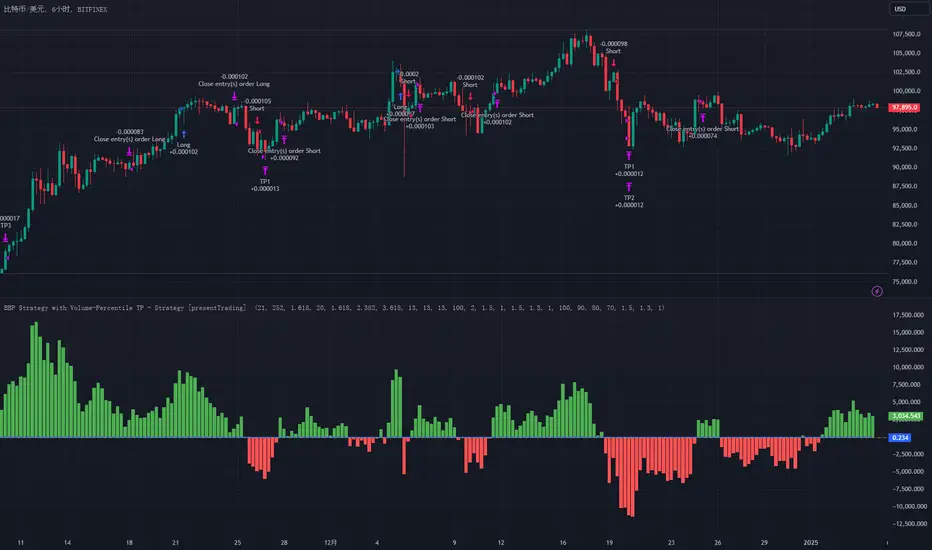
BullBear with Volume-Percentile TP - Strategy [presentTrading] Happy New Year, everyone! I hope we have a fantastic year ahead.
It's been a while since I published an open script, but it's time to return.
This strategy introduces an indicator called Bull Bear Power, combined with an advanced take-profit system, which is the main innovative and educational aspect of this script. I hope all of you find some useful insights here. Welcome to engage in meaningful exchanges. This is a versatile tool suitable for both novice and experienced traders.
█ Introduction and How it is Different
Unlike traditional strategies that rely solely on price or volume indicators, this approach combines Bull Bear Power (BBP) with volume percentile analysis to identify optimal entry and exit points. It features a dynamic take-profit mechanism based on ATR (Average True Range) multipliers adjusted by volume and percentile factors, ensuring adaptability to diverse market conditions. This multifaceted strategy not only improves signal accuracy but also optimizes risk management, distinguishing it from conventional trading methods.
BTCUSD 6hr performance
Disable the visualization of Bull Bear Power (BBP) to clearly view the Z-Score.
█ Strategy, How it Works: Detailed Explanation
The BBP Strategy with Volume-Percentile TP utilizes several interconnected components to analyze market data and generate trading signals. Here's an overview with essential equations:
🔶 Core Indicators and Calculations
1. Exponential Moving Average (EMA):
- **Purpose:** Smoothens price data to identify trends.
- **Formula:**
EMA_t = (Close_t * (2 / (lengthInput + 1))) + (EMA_(t-1) * (1 - (2 / (lengthInput + 1))))
- Usage: Baseline for Bull and Bear Power.
2. Bull and Bear Power:
- Bull Power: `BullPower = High_t - EMA_t`
- Bear Power: `BearPower = Low_t - EMA_t`
- BBP:** `BBP = BullPower + BearPower`
- Interpretation: Positive BBP indicates bullish strength, negative indicates bearish.
3. Z-Score Calculation:
- Purpose: Normalizes BBP to assess deviation from the mean.
- Formula:
Z-Score = (BBP_t - bbp_mean) / bbp_std
- Components:
- `bbp_mean` = SMA of BBP over `zLength` periods.
- `bbp_std` = Standard deviation of BBP over `zLength` periods.
- Usage: Identifies overbought or oversold conditions based on thresholds.
🔶 Volume Analysis
1. Volume Moving Average (`vol_sma`):
vol_sma = (Volume_1 + Volume_2 + ... + Volume_vol_period) / vol_period
2. Volume Multiplier (`vol_mult`):
vol_mult = Current Volume / vol_sma
- Thresholds:
- High Volume: `vol_mult > 2.0`
- Medium Volume: `1.5 < vol_mult ≤ 2.0`
- Low Volume: `1.0 < vol_mult ≤ 1.5`
🔶 Percentile Analysis
1. Percentile Calculation (`calcPercentile`):
Percentile = (Number of values ≤ Current Value / perc_period) * 100
2. Thresholds:
- High Percentile: >90%
- Medium Percentile: >80%
- Low Percentile: >70%
🔶 Dynamic Take-Profit Mechanism
1. ATR-Based Targets:
TP1 Price = Entry Price ± (ATR * atrMult1 * TP_Factor)
TP2 Price = Entry Price ± (ATR * atrMult2 * TP_Factor)
TP3 Price = Entry Price ± (ATR * atrMult3 * TP_Factor)
- ATR Calculation:
ATR_t = (True Range_1 + True Range_2 + ... + True Range_baseAtrLength) / baseAtrLength
2. Adjustment Factors:
TP_Factor = (vol_score + price_score) / 2
- **vol_score** and **price_score** are based on current volume and price percentiles.
Local performance
🔶 Entry and Exit Logic
1. Long Entry: If Z-Score crosses above 1.618, then Enter Long.
2. Short Entry: If Z-Score crosses below -1.618, then Enter Short.
3. Exiting Positions:
If Long and Z-Score crosses below 0:
Exit Long
If Short and Z-Score crosses above 0:
Exit Short
4. Take-Profit Execution:
- Set multiple exit orders at dynamically calculated TP levels based on ATR and adjusted by `TP_Factor`.
█ Trade Direction
The strategy determines trade direction using the Z-Score from the BBP indicator:
- Long Positions:
- Condition: Z-Score crosses above 1.618.
- Short Positions:
- Condition: Z-Score crosses below -1.618.
- Exiting Trades:
- Long Exit: Z-Score drops below 0.
- Short Exit: Z-Score rises above 0.
This approach aligns trades with prevailing market trends, increasing the likelihood of successful outcomes.
█ Usage
Implementing the BBP Strategy with Volume-Percentile TP in TradingView involves:
1. Adding the Strategy:
- Copy the Pine Script code.
- Paste it into TradingView's Pine Editor.
- Save and apply the strategy to your chart.
2. Configuring Settings:
- Adjust parameters like EMA length, Z-Score thresholds, ATR multipliers, volume periods, and percentile settings to match your trading preferences and asset behavior.
3. Backtesting:
- Use TradingView’s backtesting tools to evaluate historical performance.
- Analyze metrics such as profit factor, drawdown, and win rate.
4. Optimization:
- Fine-tune parameters based on backtesting results.
- Test across different assets and timeframes to enhance adaptability.
5. Deployment:
- Apply the strategy in a live trading environment.
- Continuously monitor and adjust settings as market conditions change.
█ Default Settings
The BBP Strategy with Volume-Percentile TP includes default parameters designed for balanced performance across various markets. Understanding these settings and their impact is essential for optimizing strategy performance:
Bull Bear Power Settings:
- EMA Length (`lengthInput`): 21
- **Effect:** Balances sensitivity and trend identification; shorter lengths respond quicker but may generate false signals.
- Z-Score Length (`zLength`): 252
- **Effect:** Long period for stable mean and standard deviation, reducing false signals but less responsive to recent changes.
- Z-Score Threshold (`zThreshold`): 1.618
- **Effect:** Higher threshold filters out weaker signals, focusing on significant market moves.
Take Profit Settings:
- Use Take Profit (`useTP`): Enabled (`true`)
- **Effect:** Activates dynamic profit-taking, enhancing profitability and risk management.
- ATR Period (`baseAtrLength`): 20
- **Effect:** Shorter period for sensitive volatility measurement, allowing tighter profit targets.
- ATR Multipliers:
- **Effect:** Define conservative to aggressive profit targets based on volatility.
- Position Sizes:
- **Effect:** Diversifies profit-taking across multiple levels, balancing risk and reward.
Volume Analysis Settings:
- Volume MA Period (`vol_period`): 100
- **Effect:** Longer period for stable volume average, reducing the impact of short-term spikes.
- Volume Multipliers:
- **Effect:** Determines volume conditions affecting take-profit adjustments.
- Volume Factors:
- **Effect:** Adjusts ATR multipliers based on volume strength.
Percentile Analysis Settings:
- Percentile Period (`perc_period`): 100
- **Effect:** Balances historical context with responsiveness to recent data.
- Percentile Thresholds:
- **Effect:** Defines price and volume percentile levels influencing take-profit adjustments.
- Percentile Factors:
- **Effect:** Modulates ATR multipliers based on price percentile strength.
Impact on Performance:
- EMA Length: Shorter EMAs increase sensitivity but may cause more false signals; longer EMAs provide stability but react slower to market changes.
- Z-Score Parameters:*Longer Z-Score periods create more stable signals, while higher thresholds reduce trade frequency but increase signal reliability.
- ATR Multipliers and Position Sizes: Higher multipliers allow for larger profit targets with increased risk, while diversified position sizes help in securing profits at multiple levels.
- Volume and Percentile Settings: These adjustments ensure that take-profit targets adapt to current market conditions, enhancing flexibility and performance across different volatility environments.
- Commission and Slippage: Accurate settings prevent overestimation of profitability and ensure the strategy remains viable after accounting for trading costs.
Conclusion
The BBP Strategy with Volume-Percentile TP offers a robust framework by combining BBP indicators with volume and percentile analyses. Its dynamic take-profit mechanism, tailored through ATR adjustments, ensures that traders can effectively capture profits while managing risks in varying market conditions.
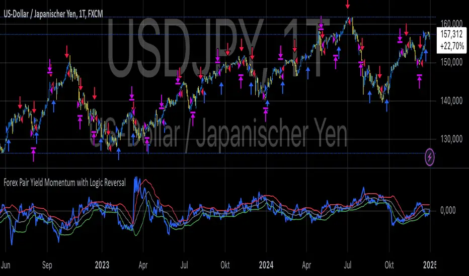
Forex Pair Yield Momentum This Pine Script strategy leverages yield differentials between the 2-year government bond yields of two countries to trade Forex pairs. Yield spreads are widely regarded as a fundamental driver of currency movements, as highlighted by international finance theories like the Interest Rate Parity (IRP), which suggests that currencies with higher yields tend to appreciate due to increased capital flows:
1. Dynamic Yield Spread Calculation:
• The strategy dynamically calculates the yield spread (yield_a - yield_b) for the chosen Forex pair.
• Example: For GBP/USD, the spread equals US 2Y Yield - UK 2Y Yield.
2. Momentum Analysis via Bollinger Bands:
• Yield momentum is computed as the difference between the current spread and its moving
Bollinger Bands are applied to identify extreme deviations:
• Long Entry: When momentum crosses below the lower band.
• Short Entry: When momentum crosses above the upper band.
3. Reversal Logic:
• An optional checkbox reverses the trading logic, allowing long trades at the upper band and short trades at the lower band, accommodating different market conditions.
4. Trade Management:
• Positions are held for a predefined number of bars (hold_periods), and each trade uses a fixed contract size of 100 with a starting capital of $20,000.
Theoretical Basis:
1. Yield Differentials and Currency Movements:
• Empirical studies, such as Clarida et al. (2009), confirm that interest rate differentials significantly impact exchange rate dynamics, especially in carry trade strategies .
• Higher-yields tend to appreciate against lower-yielding currencies due to speculative flows and demand for higher returns.
2. Bollinger Bands for Momentum:
• Bollinger Bands effectively capture deviations in yield momentum, identifying opportunities where price returns to equilibrium (mean reversion) or extends in trend-following scenarios (momentum breakout).
• As Bollinger (2001) emphasized, this tool adapts to market volatility by dynamically adjusting thresholds .
References:
1. Dornbusch, R. (1976). Expectations and Exchange Rate Dynamics. Journal of Political Economy.
2. Obstfeld, M., & Rogoff, K. (1996). Foundations of International Macroeconomics.
3. Clarida, R., Davis, J., & Pedersen, N. (2009). Currency Carry Trade Regimes. NBER.
4. Bollinger, J. (2001). Bollinger on Bollinger Bands.
5. Mendelsohn, L. B. (2006). Forex Trading Using Intermarket Analysis.
Engulfing Candlestick StrategyEver wondered whether the Bullish or Bearish Engulfing pattern works or has statistical significance? This script is for you. It works across all markets and timeframes.
The Engulfing Candlestick Pattern is a widely used technical analysis pattern that traders use to predict potential price reversals. It consists of two candles: a small candle followed by a larger one that "engulfs" the previous candle. This pattern is considered bullish when it occurs in a downtrend (bullish engulfing) and bearish when it occurs in an uptrend (bearish engulfing).
Statistical Significance of the Engulfing Pattern:
While many traders rely on candlestick patterns for making decisions, research on the statistical significance of these patterns has produced mixed results. A study by Dimitrios K. Koutoupis and K. M. Koutoupis (2014), titled "Testing the Effectiveness of Candlestick Chart Patterns in Forex Markets," indicates that candlestick patterns, including the engulfing pattern, can provide some predictive power, but their success largely depends on the market conditions and timeframe used. The researchers concluded that while some candlestick patterns can be useful, traders must combine them with other indicators or market knowledge to improve their predictive accuracy.
Another study by Brock, Lakonishok, and LeBaron (1992), "Simple Technical Trading Rules and the Stochastic Properties of Stock Returns," explores the profitability of technical indicators, including candlestick patterns, and finds that simple trading rules, such as those based on moving averages or candlestick patterns, can occasionally outperform a random walk in certain market conditions.
However, Jorion (1997), in his work "The Risk of Speculation: The Case of Technical Analysis," warns that the reliability of candlestick patterns, including the engulfing patterns, can vary significantly across different markets and periods. Therefore, it's important to use these patterns as part of a broader trading strategy that includes other risk management techniques and technical indicators.
Application Across Markets:
This script applies to all markets (e.g., stocks, commodities, forex) and timeframes, making it a versatile tool for traders seeking to explore the statistical effectiveness of the bullish and bearish engulfing patterns in their own trading.
Conclusion:
This script allows you to backtest and visualize the effectiveness of the Bullish and Bearish Engulfing patterns across any market and timeframe. While the statistical significance of these patterns may vary, the script provides a clear framework for evaluating their performance in real-time trading conditions. Always remember to combine such patterns with other risk management strategies and indicators to enhance their predictive power.

Daytrading ES Wick Length StrategyThis Pine Script strategy calculates the combined length of upper and lower wicks of candlesticks and uses a customizable moving average (MA) to identify potential long entry points. The strategy compares the total wick length to the MA with an added offset. If the wick length exceeds the offset-adjusted MA, the strategy enters a long position. The position is automatically closed after a user-defined holding period.
Key Features:
1. Calculates the sum of upper and lower wicks for each candlestick.
2. Offers four types of moving averages (SMA, EMA, WMA, VWMA) for analysis.
3. Allows the user to set a customizable MA length and an offset to shift the MA.
4. Automatically exits positions after a specified number of bars.
5. Visualizes the wick length as a histogram and the offset-adjusted MA as a line.
References:
• Candlestick wick analysis: Nison, S. (1991). Japanese Candlestick Charting Techniques.
• Moving averages: Brock, W., Lakonishok, J., & LeBaron, B. (1992). “Simple Technical Trading Rules and the Stochastic Properties of Stock Returns”. Journal of Finance.
This strategy is suitable for identifying candlesticks with significant volatility and long wicks, which can indicate potential trend reversals or continuations.
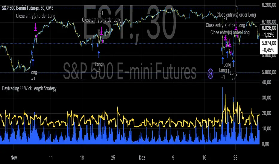
Up Gap Strategy with DelayThis strategy, titled “Up Gap Strategy with Delay,” is based on identifying up gaps in the price action of an asset. A gap is defined as the percentage difference between the current bar’s open price and the previous bar’s close price. The strategy triggers a long position if the gap exceeds a user-defined threshold and includes a delay period before entering the position. After entering, the position is held for a set number of periods before being closed.
Key Features:
1. Gap Threshold: The strategy defines an up gap when the gap size exceeds a specified threshold (in percentage terms). The gap threshold is an input parameter that allows customization based on the user’s preference.
2. Delay Period: After the gap occurs, the strategy waits for a delay period before initiating a long position. This delay can help mitigate any short-term volatility that might occur immediately after the gap.
3. Holding Period: Once the position is entered, it is held for a user-defined number of periods (holdingPeriods). This is to capture the potential post-gap trend continuation, as gaps often indicate strong directional momentum.
4. Gap Plotting: The strategy visually plots up gaps on the chart by placing a green label beneath the bar where the gap condition is met. Additionally, the background color turns green to highlight up-gap occurrences.
5. Exit Condition: The position is exited after the defined holding period. The strategy ensures that the position is closed after this time, regardless of whether the price is in profit or loss.
Scientific Background:
The gap theory has been widely studied in financial literature and is based on the premise that gaps in price often represent areas of significant support or resistance. According to research by Kaufman (2002), gaps in price action can be indicators of future price direction, particularly when they occur after a period of consolidation or a trend reversal. Moreover, Gaps and their Implications in Technical Analysis (Murphy, 1999) highlights that gaps can reflect imbalances between supply and demand, leading to high momentum and potential price continuation or reversal.
In trading strategies, utilizing gaps with specific conditions, such as delay and holding periods, can enhance the ability to capture significant price moves. The strategy’s delay period helps avoid potential market noise immediately after the gap, while the holding period seeks to capitalize on the price continuation that often follows gap formation.
This methodology aligns with momentum-based strategies, which rely on the persistence of trends in financial markets. Several studies, including Jegadeesh & Titman (1993), have documented the existence of momentum effects in stock prices, where past price movements can be predictive of future returns.
Conclusion:
This strategy incorporates gap detection and momentum principles, supported by empirical research in technical analysis, to attempt to capitalize on price movements following significant gaps. By waiting for a delay period and holding the position for a specified time, it aims to mitigate the risk associated with early volatility while maximizing the potential for sustained price moves.