MOR+ [JJumbo]Midnight Opening Range (MOR)
Designed for opening range and ICT traders
- Midnight Opening Range Analysis
Accurate Price Benchmarking: Captures the essential price movements at the midnight
opening, providing a solid foundation for your trading decisions.
- RTH Candles Shadowing
Enhanced Visualization: Displays Regular Trading Hours (RTH) candle shadows, allowing you to
clearly see price fluctuations and trends during active trading periods.
- Standard Deviations
Incorporates standard deviation calculations to measure market
volatility, helping you identify potential breakout and reversal points with greater
confidence.
- Midnight Opening Price Reference
Strategic Entry Points: Highlights the midnight opening price, serving as a critical reference
level.
- Comprehensive Range Points Calculation Table
Detailed Analysis: Features a dynamic table that calculates and displays range points,
enabling you to track and analyze key price levels effortlessly.
Desvio Padrão

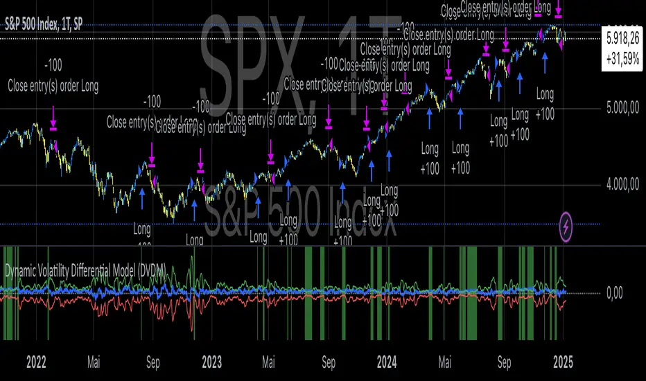
Dynamic Volatility Differential Model (DVDM)The Dynamic Volatility Differential Model (DVDM) is a quantitative trading strategy designed to exploit the spread between implied volatility (IV) and historical (realized) volatility (HV). This strategy identifies trading opportunities by dynamically adjusting thresholds based on the standard deviation of the volatility spread. The DVDM is versatile and applicable across various markets, including equity indices, commodities, and derivatives such as the FDAX (DAX Futures).
Key Components of the DVDM:
1. Implied Volatility (IV):
The IV is derived from options markets and reflects the market’s expectation of future price volatility. For instance, the strategy uses volatility indices such as the VIX (S&P 500), VXN (Nasdaq 100), or RVX (Russell 2000), depending on the target market. These indices serve as proxies for market sentiment and risk perception (Whaley, 2000).
2. Historical Volatility (HV):
The HV is computed from the log returns of the underlying asset’s price. It represents the actual volatility observed in the market over a defined lookback period, adjusted to annualized levels using a multiplier of \sqrt{252} for daily data (Hull, 2012).
3. Volatility Spread:
The difference between IV and HV forms the volatility spread, which is a measure of divergence between market expectations and actual market behavior.
4. Dynamic Thresholds:
Unlike static thresholds, the DVDM employs dynamic thresholds derived from the standard deviation of the volatility spread. The thresholds are scaled by a user-defined multiplier, ensuring adaptability to market conditions and volatility regimes (Christoffersen & Jacobs, 2004).
Trading Logic:
1. Long Entry:
A long position is initiated when the volatility spread exceeds the upper dynamic threshold, signaling that implied volatility is significantly higher than realized volatility. This condition suggests potential mean reversion, as markets may correct inflated risk premiums.
2. Short Entry:
A short position is initiated when the volatility spread falls below the lower dynamic threshold, indicating that implied volatility is significantly undervalued relative to realized volatility. This signals the possibility of increased market uncertainty.
3. Exit Conditions:
Positions are closed when the volatility spread crosses the zero line, signifying a normalization of the divergence.
Advantages of the DVDM:
1. Adaptability:
Dynamic thresholds allow the strategy to adjust to changing market conditions, making it suitable for both low-volatility and high-volatility environments.
2. Quantitative Precision:
The use of standard deviation-based thresholds enhances statistical reliability and reduces subjectivity in decision-making.
3. Market Versatility:
The strategy’s reliance on volatility metrics makes it universally applicable across asset classes and markets, ensuring robust performance.
Scientific Relevance:
The strategy builds on empirical research into the predictive power of implied volatility over realized volatility (Poon & Granger, 2003). By leveraging the divergence between these measures, the DVDM aligns with findings that IV often overestimates future volatility, creating opportunities for mean-reversion trades. Furthermore, the inclusion of dynamic thresholds aligns with risk management best practices by adapting to volatility clustering, a well-documented phenomenon in financial markets (Engle, 1982).
References:
1. Christoffersen, P., & Jacobs, K. (2004). The importance of the volatility risk premium for volatility forecasting. Journal of Financial and Quantitative Analysis, 39(2), 375-397.
2. Engle, R. F. (1982). Autoregressive conditional heteroskedasticity with estimates of the variance of United Kingdom inflation. Econometrica, 50(4), 987-1007.
3. Hull, J. C. (2012). Options, Futures, and Other Derivatives. Pearson Education.
4. Poon, S. H., & Granger, C. W. J. (2003). Forecasting volatility in financial markets: A review. Journal of Economic Literature, 41(2), 478-539.
5. Whaley, R. E. (2000). The investor fear gauge. Journal of Portfolio Management, 26(3), 12-17.
This strategy leverages quantitative techniques and statistical rigor to provide a systematic approach to volatility trading, making it a valuable tool for professional traders and quantitative analysts.
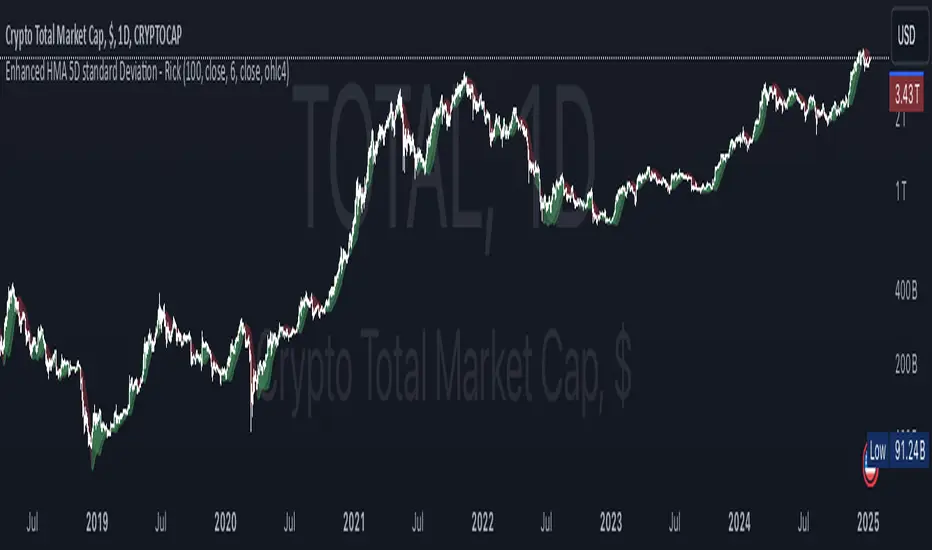
Enhanced HMA 5D standard Deviation - RickSimple hull moving average enhanced with standard deviation bands calculated over a 5 day period to account for volatility in ranging periods.
Possibility to choose the source of the hull calculation, as well as the source to use as threshold for long and short signal.
Two different types of visualization: candle coloring or moving average.
Prime Bands [ChartPrime]The Prime Standard Deviation Bands indicator uses custom-calculated bands based on highest and lowest price values over specific period to analyze price volatility and trend direction. Traders can set the bands to 1, 2, or 3 standard deviations from a central base, providing a dynamic view of price behavior in relation to volatility. The indicator also includes color-coded trend signals, standard deviation labels, and mean reversion signals, offering insights into trend strength and potential reversal points.
⯁ KEY FEATURES AND HOW TO USE
⯌ Standard Deviation Bands :
The indicator plots upper and lower bands based on standard deviation settings (1, 2, or 3 SDs) from a central base, allowing traders to visualize volatility and price extremes. These bands can be used to identify overbought and oversold conditions, as well as potential trend reversals.
Example of 3-standard-deviation bands around price:
⯌ Dynamic Trend Indicator :
The midline of the bands changes color based on trend direction. If the midline is rising, it turns green, indicating an uptrend. When the midline is falling, it turns orange, suggesting a downtrend. This color coding provides a quick visual reference to the current trend.
Trend color examples for rising and falling midlines:
⯌ Standard Deviation Labels :
At the end of the bands, the indicator displays labels with price levels for each standard deviation level (+3, 0, -3, etc.), helping traders quickly reference where price is relative to its statistical boundaries.
Price labels at each standard deviation level on the chart:
⯌ Mean Reversion Signals :
When price moves beyond the upper or lower bands and then reverts back inside, the indicator plots mean reversion signals with diamond icons. These signals indicate potential reversal points where the price may return to the mean after extreme moves.
Example of mean reversion signals near bands:
⯌ Standard Deviation Scale on Chart :
A visual scale on the right side of the chart shows the current price position in relation to the bands, expressed in standard deviations. This scale provides an at-a-glance view of how far price has deviated from the mean, helping traders assess risk and volatility.
⯁ USER INPUTS
Length : Sets the number of bars used in the calculation of the bands.
Standard Deviation Level : Allows selection of 1, 2, or 3 standard deviations for upper and lower bands.
Colors : Customize colors for the uptrend and downtrend midline indicators.
⯁ CONCLUSION
The Prime Standard Deviation Bands indicator provides a comprehensive view of price volatility and trend direction. Its customizable bands, trend coloring, and mean reversion signals allow traders to effectively gauge price behavior, identify extreme conditions, and make informed trading decisions based on statistical boundaries.

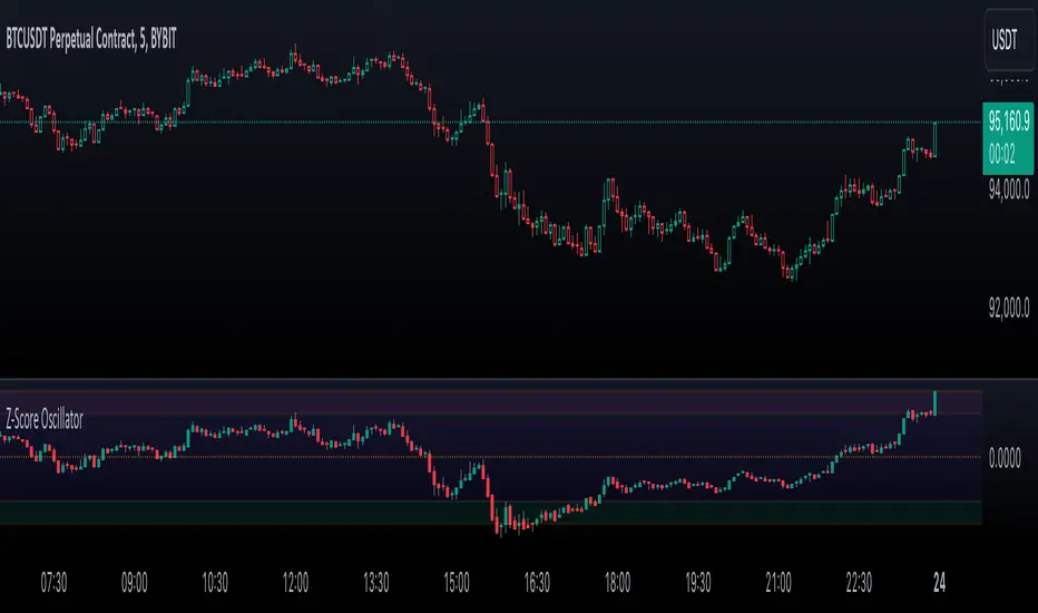
Enhanced Price Z-Score OscillatorThe Enhanced Price Z-Score Oscillator by tkarolak is a powerful tool that transforms raw price data into an easy-to-understand statistical visualization using Z-Score-derived candlesticks. Simply put, it shows how far prices stray from their average in terms of standard deviations (Z-Scores), helping traders identify when prices are unusually high (overbought) or unusually low (oversold).
The indicator’s default feature displays Z-Score Candlesticks, where each candle reflects the statistical “distance” of the open, high, low, and close prices from their average. This creates a visual map of market extremes and potential reversal points. For added flexibility, you can also switch to Z-Score line plots based on either Close prices or OHLC4 averages.
With clear threshold lines (±2σ and ±3σ) marking moderate and extreme price deviations, and color-coded zones to highlight overbought and oversold areas, the oscillator simplifies complex statistical concepts into actionable trading insights.
RSI BB StdDev SignalOverview
The RSI BB StdDev Signal Indicator is a powerful tool designed to enhance your trading strategy by combining the Relative Strength Index (RSI) with Bollinger Bands (BB). This unique combination allows traders to identify potential buy and sell signals more accurately by leveraging the strengths of both indicators. The RSI helps in identifying overbought and oversold conditions, while the Bollinger Bands provide a dynamic range to assess volatility and potential price reversals.
Key Features
— RSI Calculation: The indicator calculates the RSI based on user-defined parameters, allowing for customization to fit different trading styles.
— Bollinger Bands Integration: The RSI values are smoothed using a moving average, and Bollinger Bands are applied to this smoothed RSI to generate buy and sell signals.
— Divergence Detection: The indicator includes an optional feature to detect and alert on bullish and bearish divergences between the RSI and price action.
— Customizable Alerts: Users can set up alerts for buy and sell signals, as well as for divergences, ensuring they never miss a trading opportunity.
— Visual Aids: The indicator plots the RSI, Bollinger Bands, and signals on the chart, making it easy to visualize and interpret the data.
How It Works
1. RSI Calculation:
— The RSI is calculated using the change in the source input (default is close price) over a specified period.
— The RSI values are then plotted on the chart with customizable overbought and oversold levels.
2. Smoothing and Bollinger Bands:
— The RSI values are smoothed using a moving average (SMA, EMA, SMMA, WMA, VWMA) selected by the user.
— Bollinger Bands are applied to the smoothed RSI to create dynamic upper and lower bands.
3. Signal Generation:
—Buy signals are generated when the RSI crosses above the lower Bollinger Band.
—Sell signals are generated when the RSI crosses below the upper Bollinger Band.
—These signals are plotted on both the RSI pane and the main price chart for easy reference.
4. Divergence Detection:
— The indicator can detect and alert on regular bullish and bearish divergences between the RSI and price action.
— Bullish divergences occur when the price makes a lower low, but the RSI makes a higher low.
— Bearish divergences occur when the price makes a higher high, but the RSI makes a lower high.
Usage
1. Setting Up:
— Add the indicator to your TradingView chart.
— Customize the RSI length, source, and other parameters in the settings panel.
— Enable or disable the divergence detection based on your trading strategy.
2. Interpreting Signals:
— Use the buy and sell signals generated by the RSI crossing the Bollinger Bands as potential entry and exit points.
— Pay attention to divergences for additional confirmation of trend reversals.
3. Alerts:
— Set up alerts for buy and sell signals to receive notifications in real-time.
— Enable divergence alerts to be notified of potential trend reversals.
Conclusion
The RSI BB StdDev Signal Indicator is a comprehensive tool that combines the strengths of the RSI and Bollinger Bands to provide traders with more accurate and reliable signals. Whether you are a beginner or an experienced trader, this indicator can enhance your trading strategy by offering clear visual cues and customizable alerts.
Note
This indicator is provided with open-source code, allowing users to understand its logic and customize it further if needed. The detailed description and customizable settings ensure that traders of all levels can benefit from its unique features.

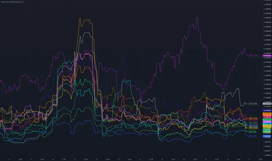
Crypto Price Volatility Range# Cryptocurrency Price Volatility Range Indicator
This TradingView indicator is a visualization tool for tracking historical volatility across multiple major cryptocurrencies.
## Features
- Real-time volatility tracking for 14 major cryptocurrencies
- Customizable period and standard deviation multiplier
- Individual color coding for each currency pair
- Optional labels showing current volatility values in percentage
## Supported Cryptocurrencies
- Bitcoin (BTC)
- Ethereum (ETH)
- Avalanche (AVAX)
- Dogecoin (DOGE)
- Hype (HYPE)
- Ripple (XRP)
- Binance Coin (BNB)
- Cardano (ADA)
- Tron (TRX)
- Chainlink (LINK)
- Shiba Inu (SHIB)
- Toncoin (TON)
- Sui (SUI)
- Stellar (XLM)
## Settings
- **Period**: Timeframe for volatility calculation (default: 20)
- **Standard Deviation Multiplier**: Multiplier for standard deviation (default: 1.0)
- **Show Labels**: Toggle label display on/off
## Calculation Method
The indicator calculates volatility using the following method:
1. Calculate daily logarithmic returns
2. Compute standard deviation over the specified period
3. Annualize (multiply by √252)
4. Convert to percentage (×100)
## Usage
1. Add the indicator to your TradingView chart
2. Adjust parameters as needed
3. Monitor volatility lines for each cryptocurrency
4. Enable labels to see precise current volatility values
## Notes
- This indicator displays in a separate window, not as an overlay
- Volatility values are annualized
- Data for each currency pair is sourced from USD pairs
Market Anomaly Detector (MAD)Market Anomaly Detector (MAD) Indicator - Detailed Description:
The Market Anomaly Detector (MAD) Indicator is a unique tool designed to identify potential market anomalies by combining several price action-based and momentum indicators. This indicator is especially useful for traders who seek to identify significant market shifts and anomalies before they become visible in conventional technical indicators.
Key Features of the MAD Indicator:
1. Z-Score Threshold for Anomaly Detection:
• The Z-Score measures how far a current price is from its average over a defined period, normalized by standard deviation. This allows the MAD indicator to detect outliers or anomalies in price movements.
• By adjusting the Z-Score Threshold, traders can tune the sensitivity of the indicator to capture only the most significant price deviations, filtering out noise and reducing false signals.
2. Volume and Liquidity Filter:
• Volume is a key indicator of market participation and sentiment. The MAD Indicator uses a volume multiplier to assess when price movements are supported by sufficient trading volume.
• A volume spike is identified when the current volume exceeds the average volume by a certain multiplier. This ensures that only high-confidence signals are generated, particularly useful for spotting trend reversals and breakout opportunities.
3. Signal Cooldown Period:
• To prevent overfitting and reduce false signals, a signal cooldown period is implemented. Once a buy or sell signal is triggered, the indicator waits for a specified number of bars (e.g., 5) before triggering another signal, even if the price action meets the criteria for a new signal. This helps maintain a cleaner trading environment and avoids confusion when the market is volatile.
4. Upper and Lower Bands for Trend Confirmation:
• The MAD Indicator uses bands based on the mean price and standard deviation, similar to Bollinger Bands. These upper and lower bands help to define the expected price range for a given period, indicating overbought or oversold conditions.
• The combination of Z-Score, volume, and band analysis helps pinpoint when the price breaks out of expected ranges, providing early warning signs for potential market shifts.
5. Trend Confirmation from Higher Timeframes:
• The MAD Indicator includes a multi-timeframe approach to trend confirmation, using the 50-period EMA on a higher timeframe (e.g., 1-hour chart). This ensures that signals are aligned with the overall market trend, enhancing the reliability of buy and sell signals.
How It Works:
• The MAD Indicator continuously monitors price action, volume, and statistical anomalies, using the Z-Score to determine when the price is significantly deviating from its historical average.
• When the price breaks above the upper band and a bullish anomaly is detected, a buy signal is generated. (Green Background)
• Similarly, when the price breaks below the lower band and a bearish anomaly is detected, a sell signal is triggered. (Red Background
• By filtering signals based on volume and using the cooldown period, the MAD Indicator ensures that only high-quality trades are signaled.
How to Use the MAD Indicator:
• Buy Signal: Occurs when the price breaks above the upper band and there is a significant deviation from the mean (bullish anomaly).
• Sell Signal: Occurs when the price breaks below the lower band and there is a significant deviation from the mean (bearish anomaly).
• Volume Confirmation: Ensure that the buy/sell signals are supported by a volume spike, indicating strong market participation.
• Signal Cooldown Period: After a signal is triggered, the indicator waits for the cooldown period to avoid triggering multiple signals in quick succession.
Why It’s Worth Paying For:
The MAD Indicator combines advanced statistical analysis (Z-Score), price action, and volume analysis to identify market anomalies and breakouts before they are visible on standard indicators. By leveraging the power of mean reversion and statistical anomalies, this tool provides traders with high-confidence signals that can lead to profitable trades, especially in volatile markets. The integration of a multi-timeframe trend filter ensures that signals are aligned with the overall market trend, reducing the likelihood of false breakouts.
This indicator is ideal for trend-following traders looking for high-probability entries and mean-reversion traders aiming to capture price deviations. The signal cooldown period and volume filter provide an additional layer of precision, ensuring that you only act on the strongest market signals.

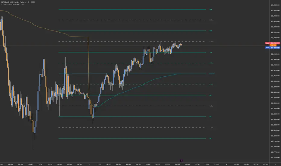
VWAP Trend with Standard Deviation & MidlinesThis indicator is a sophisticated VWAP (Volume Weighted Average Price) tool with multiple features:
Core Functionality:
1. Calculates a primary VWAP line that changes color based on trend direction (green when rising, red when falling)
2. Creates multiple standard deviation bands around the VWAP at customizable distances
3. Resets calculations at either:
- New York session start time (configurable, default 9:30 AM)
- Daily start time
- Can be hidden on daily/weekly/monthly timeframes if desired
Band Structure:
- Band 1 (innermost): ±1 standard deviation
- Band 2 (middle): ±2 standard deviations
- Band 3 (outermost): ±3 standard deviations
- Midlines at 0.5σ intervals between bands
- All bands can be individually enabled/disabled
Customization Options:
1. Band calculation modes:
- Standard Deviation based
- Percentage based
2. Visual settings:
- Customizable colors for all elements
- Adjustable line widths
- Optional labels with configurable size
- Optional extension lines
- Label position adjustment
3. Source data selection (default: HLC3 - High, Low, Close average)
Common Uses:
- Identifying potential support/resistance levels
- Measuring price volatility
- Spotting mean reversion opportunities
- Trading range analysis
- Trend direction confirmation
The indicator essentially creates a dynamic support/resistance structure that adapts to market volatility and volume, making it useful for both intraday and swing trading strategies.
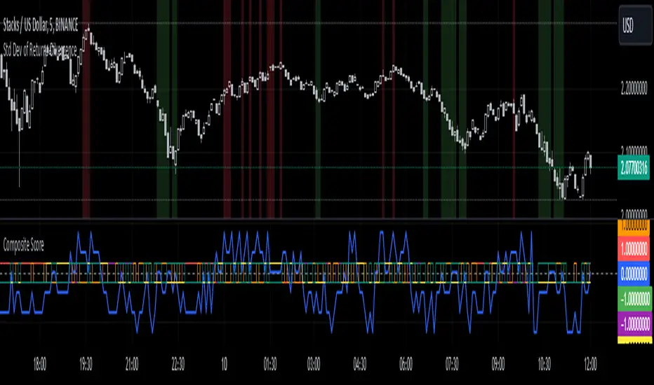
Standard Deviation of Returns: DivergencePurpose:
The "Standard Deviation of Returns: Divergence" indicator is designed to help traders identify potential trend reversals or continuation signals by analyzing divergences between price action and the statistical volatility of returns. Divergences can signal weakening momentum in the prevailing trend, offering insight into potential buying or selling opportunities.
Key Components
1. Returns Calculation:
* The indicator uses logarithmic returns (log(close / close )) to measure relative price changes in a normalized manner.
* Log returns are more effective than simple price differences when analyzing data across varying price levels, as they account for percentage-based changes.
2. Standard Deviation of Returns:
* The script computes the standard deviation of returns over a user-defined lookback period (ta.stdev(returns, lookback)).
* Standard deviation measures the dispersion of returns around their average, effectively quantifying market volatility.
* A higher standard deviation indicates increased volatility, while lower standard deviation reflects a calmer market.
3. Price Action:
* Detects higher highs (new peaks in price) and lower lows (new troughs in price) over the lookback period.
* Price trends are compared to the behavior of the standard deviation.
4. Divergence Detection:
A divergence occurs when price action (higher highs or lower lows) is not confirmed by a corresponding movement in standard deviation:
Bullish Divergence: Price makes a lower low, but the standard deviation does not, signaling potential upward momentum.
Bearish Divergence: Price makes a higher high, but the standard deviation does not, signaling potential downward momentum.
5. Visual Cues:
The script highlights divergence regions directly on the chart:
Green Background: Indicates a bullish divergence (potential buy signal).
Red Background: Indicates a bearish divergence (potential sell signal).
How It Works
Inputs:
* The user specifies the lookback period (lookback) for calculating the standard deviation and detecting divergences.
Calculation:
* Each bar’s returns are computed and used to calculate the standard deviation over the specified lookback period.
* The indicator evaluates price highs/lows and compares these with the highest and lowest values of the standard deviation within the same lookback period.
Highlight of Divergences:
When divergences are detected:
Bullish Divergence: The background of the chart is shaded green.
Bearish Divergence: The background of the chart is shaded red.
Trading Application
Bullish Divergence:
* Occurs when the market is oversold, or downward momentum is weakening.
* Suggests a potential reversal to an uptrend, signaling a buying opportunity.
Bearish Divergence:
* Occurs when the market is overbought, or upward momentum is weakening.
* Suggests a potential reversal to a downtrend, signaling a selling opportunity.
Contextual Use:
* Use this indicator in conjunction with other technical tools like RSI, MACD, or moving averages to confirm signals.
* Effective in volatile or ranging markets to help anticipate shifts in momentum.
Summary
The "Standard Deviation of Returns: Divergence" indicator is a robust tool for spotting divergences that can signal weakening market trends. It combines statistical volatility with price action analysis to highlight key areas of potential reversals. By integrating this tool into your trading strategy, you can gain additional confirmation for entries or exits while keeping a close watch on momentum shifts.
Disclaimer: This is not a financial advise; please consult your financial advisor for personalized advice.
BTCUSD Momentum After Abnormal DaysThis indicator identifies abnormal days in the Bitcoin market (BTCUSD) based on daily returns exceeding specific thresholds defined by a statistical approach. It is inspired by the findings of Caporale and Plastun (2020), who analyzed the cryptocurrency market's inefficiencies and identified exploitable patterns, particularly around abnormal returns.
Key Concept:
Abnormal Days:
Days where the daily return significantly deviates (positively or negatively) from the historical average.
Positive abnormal days: Returns exceed the mean return plus k times the standard deviation.
Negative abnormal days: Returns fall below the mean return minus k times the standard deviation.
Momentum Effect:
As described in the academic paper, on abnormal days, prices tend to move in the direction of the abnormal return until the end of the trading day, creating momentum effects. This can be leveraged by traders for profit opportunities.
How It Works:
Calculation:
The script calculates the daily return as the percentage difference between the open and close prices. It then derives the mean and standard deviation of returns over a configurable lookback period.
Thresholds:
The script dynamically computes upper and lower thresholds for abnormal days using the mean and standard deviation. Days exceeding these thresholds are flagged as abnormal.
Visualization:
The mean return and thresholds are plotted as dynamic lines.
Abnormal days are visually highlighted with transparent green (positive) or red (negative) backgrounds on the chart.
References:
This indicator is based on the methodology discussed in "Momentum Effects in the Cryptocurrency Market After One-Day Abnormal Returns" by Caporale and Plastun (2020). Their research demonstrates that hourly returns during abnormal days exhibit a strong momentum effect, moving in the same direction as the abnormal return. This behavior contradicts the efficient market hypothesis and suggests profitable trading opportunities.
"Prices tend to move in the direction of abnormal returns till the end of the day, which implies the existence of a momentum effect on that day giving rise to exploitable profit opportunities" (Caporale & Plastun, 2020).

Dema Percentile Standard DeviationDema Percentile Standard Deviation
The Dema Percentile Standard Deviation indicator is a robust tool designed to identify and follow trends in financial markets.
How it works?
This code is straightforward and simple:
The price is smoothed using a DEMA (Double Exponential Moving Average).
Percentiles are then calculated on that DEMA.
When the closing price is below the lower percentile, it signals a potential short.
When the closing price is above the upper percentile and the Standard Deviation of the lower percentile, it signals a potential long.
Settings
Dema/Percentile/SD/EMA Length's: Defines the period over which calculations are made.
Dema Source: The source of the price data used in calculations.
Percentiles: Selects the type of percentile used in calculations (options include 60/40, 60/45, 55/40, 55/45). In these settings, 60 and 55 determine percentile for long signals, while 45 and 40 determine percentile for short signals.
Features
Fully Customizable
Fully Customizable: Customize colors to display for long/short signals.
Display Options: Choose to show long/short signals as a background color, as a line on price action, or as trend momentum in a separate window.
EMA for Confluence: An EMA can be used for early entries/exits for added signal confirmation, but it may introduce noise—use with caution!
Built-in Alerts.
Indicator on Diffrent Assets
INDEX:BTCUSD 1D Chart (6 high 56 27 60/45 14)
CRYPTO:SOLUSD 1D Chart (24 open 31 20 60/40 14)
CRYPTO:RUNEUSD 1D Chart (10 close 56 14 60/40 14)
Remember no indicator would on all assets with default setting so FAFO with setting to get your desired signal.
Standard Deviation OscillatorStandard Deviation Oscillator (STDEV OSC) v1.1
Description
The Standard Deviation Oscillator transforms traditional volatility measurements into a dynamic oscillator that fluctuates between 0 and 100. This advanced technical analysis tool helps traders identify periods of extreme volatility and potential market turning points.
Features
Normalized volatility readings (0-100 scale)
Dynamic color changes based on volatility levels
Customizable overbought/oversold thresholds
Built-in alert conditions
Adaptive calculation using rolling windows
Clean, professional visualization
Indicator Parameters
Length: 20; Calculation period for standard deviation
Source: close; Price source for calculations
Overbought Level: 70; Upper threshold for high volatility
Oversold Level: 30; Lower threshold for low volatility
Visual Components
- Main Oscillator Line: Changes color based on current level
- Red: Above overbought level
- Green: Below oversold level
- Blue: Normal range
- Reference Lines:
- Overbought level (default: 70)
- Oversold level (default: 30)
- Middle line (50)
Alert Conditions
1. Volatility High Alert
- Triggers when oscillator crosses above the overbought level
- Useful for identifying potential market tops or breakout scenarios
2. Volatility Low Alert
- Triggers when oscillator crosses below the oversold level
- Helps identify potential market bottoms or consolidation periods
Risk Adjustment Tool
- Scale position sizes inversely to oscillator readings
- Reduce exposure during extremely high volatility periods
- Increase position sizes during normal volatility conditions
Best Practices
1. Timeframe Selection
- Best suited for 1H, 4H, and Daily charts
- Adjust length parameter based on timeframe
2. Confirmation
- Use in conjunction with trend indicators
- Confirm signals with price action patterns
- Consider overall market context
3. Parameter Optimization
- Backtest different length settings
- Adjust overbought/oversold levels based on asset
- Consider market conditions when setting alerts
Technical Notes
- Built in PineScript v5
- Optimized for TradingView platform
- Uses rolling window calculations for better adaptability
- Compatible with all trading instruments
- Minimal performance impact on charts
Version History
- v1.1: Added dynamic coloring, customizable levels, and alert conditions
- v1.0: Initial release with basic oscillator functionality
Disclaimer
This technical indicator is provided for educational and informational purposes only. Past performance is not indicative of future results. Always conduct thorough testing and use proper risk management techniques.
---
Tags: #TechnicalAnalysis #Volatility #Trading #Oscillator #TradingView #PineScript

Standard Deviation-Based Fibonacci Band by zdmre This indicator is designed to better understand market dynamics by focusing on standard deviation and the Fibonacci sequence. This indicator includes the following components to assist investors in analyzing price movements:
Weighted Moving Average (WMA) : The indicator creates a central band by utilizing the weighted moving average of standard deviation. WMA provides a more current and accurate representation by giving greater weight to recent prices. This central band offers insights into the general trend of the market, helping to identify potential buying and selling opportunities.
Fibonacci Bands : The Fibonacci bands located above and below the central band illustrate potential support and resistance levels for prices. These bands enable investors to pinpoint areas where the price may exhibit indecisiveness. When prices move within these bands, it may be challenging for investors to discern the market's preferred direction.
Indecisiveness Representation : When prices fluctuate between the Fibonacci bands, they may reflect a state of indecisiveness. This condition is critical for identifying potential reversal points and trend changes. Investors can evaluate these periods of indecisiveness to develop suitable buying and selling strategies.
This indicator is designed to assist investors in better analyzing market trends and supporting their decision-making processes. The integration of standard deviation and the Fibonacci sequence offers a new perspective on understanding market movements.
#DYOR

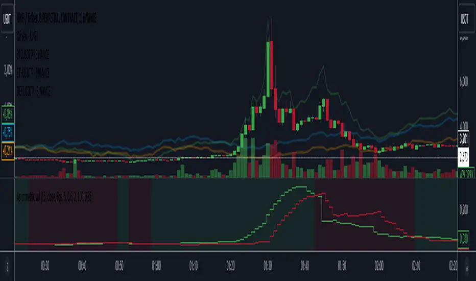
Asymmetric volatilityThe "Asymmetric Volatility" indicator is designed to visualize the differences in volatility between upward and downward price movements of a selected instrument. It operates on the principle of analyzing price movements over a specified time period, with particular focus on the symmetrical evaluation of both price rises and falls.
User Parameters:
- Length: This parameter specifies the number of bars (candles) used to calculate the average volatility. The larger the value, the longer the time period, and the smoother the volatility data will be.
- Source: This represents the input data for the indicator calculations. By default, the close value of each bar is used, but the user can choose another data source (such as open, high, low, or any custom value).
Operational Algorithm:
1. Movement Calculation:
- UpMoves: Computed as the positive difference between the current bar value and the previous bar value, if it is greater than zero.
- DownMoves: Computed as the positive difference between the previous bar value and the current bar value, if it is greater than zero.
2. Volatility Calculation:
- UpVolatility: This is the arithmetic mean of the UpMoves values over the specified period.
- DownVolatility: This is the arithmetic mean of the DownMoves values over the specified period.
3. Graphical Representation:
- The indicator displays two plots: upward and downward volatility, represented by green and red lines, respectively.
- The background color changes based on which volatility is dominant: a green background indicates that upward volatility prevails, while a red background indicates downward volatility.
The indicator allows traders to quickly assess in which direction the market is more volatile at the moment, which can be useful for making trading decisions and evaluating the current market situation.
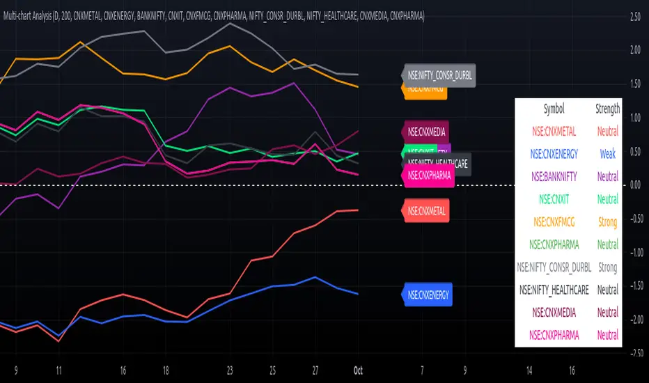
Multi-Chart Relative Strength Oscillator[ChartGalaxy]The Multi-Chart Relative Strength Oscillator is a powerful tool designed to compare the relative strength of up to 10 different market symbols (such as indices, stocks, or commodities). By normalizing each symbol's performance, this oscillator highlights which symbols are showing strength or weakness relative to each other over a selected time period.
Key Features:
Multiple Symbols Comparison: Compare up to 10 different symbols simultaneously.
Oscillator Calculation: Each symbol's price is normalized and converted into an oscillator, allowing for easy comparison of relative strength
Custom Timeframes: Choose any resolution (e.g., daily, weekly) for analyzing the symbols.
Dynamic Labeling: Each symbol is labeled on the chart for easy identification with color-coded labels that match the plotted lines.
Strength Classification: Symbols are classified as "Strong", "Neutral", or "Weak" based on their performance relative to others.
Optional Symbol Table: A table of the symbols and their strength is displayed on the chart, giving a quick overview of the current market conditions.
How it Works:
Symbol Input: The user can input up to 10 market symbols (such as indices or stocks) they wish to compare.
Oscillator Calculation: The indicator calculates the normalized value of each symbol over the selected time period, adjusting for standard deviation to create a relative strength oscillator.
Visual Comparison: The symbols are plotted as oscillating lines on the chart, color-coded for easy differentiation. Additionally, labels appear on the right side of each plot to indicate the symbol.
Strength Assessment: Each symbol is classified as Strong/Weal/Neutral
Use Cases:
Sector Rotation Analysis: Compare different sectors (e.g., Energy, Technology, Healthcare) to see which sectors are gaining or losing relative strength.
Asset Comparison: Analyze a group of stocks, commodities, or other assets to determine which are outperforming or underperforming.
Market Overview: Get a broad overview of the market by comparing key indices and sectors to gauge the overall market sentiment.
Customization Options:
Resolution Selection: Users can select their preferred timeframe for analysis (e.g., daily, weekly).
Custom Symbol Selection: Input any symbol supported by TradingView to compare performance.
Visual Clarity: Each symbol is plotted with distinct colors, and a label with the symbol’s name appears alongside the chart, making it easy to identify each line.
This indicator is ideal for traders looking to conduct sector analysis, asset comparison, or relative strength studies across multiple symbols, providing them with an intuitive and easy-to-read visual tool.
Outlier changes alertAn indicator that calculates click (price change), percentage change, and Z-score changes while displaying outliers based on defined ranges.
Outlier Detection:
Mark outliers (for price, percentage, Z-score) based on user-defined thresholds. For example, any price movement exceeding a certain Z-score or percentage change could be marked as an outlier and displayed on chart.
Indicator Overview:
1. Click (Price Change):
Calculate the absolute price change from one period to another (e.g., from the current closing price to the previous closing price).
2. Percentage Change:
Calculate the percentage price change over a specific period, showing how much the price has changed in relative terms compared to the previous price.
3. Z-Score:
Compute the Z-score to standardize the price change relative to its historical average and standard deviation. The Z-score helps in detecting whether a price movement is an outlier or falls within a normal range of volatility.

Standard Deviation based Upper Lower RangeThis script makes use of historical data for finding the standard deviation on daily returns. Based on the mean and standard deviation, the upper and lower range for the stock is shown upto 2x standard deviation. These bounds can be treated as volatility range for the next n trading sessions. This volatility is based on historical data. Users can change the lookback historical period, and can also set the time period (days) for upcoming trading sessions.
This indicator can be useful in determining stoploss and target levels along with the traditional support/resistance levels. It can also be useful in option trading where one needs to determine a range beyond which it is safe to sell an option.
A range of 1 SD has around 65% to 68% probability that it will not be breached. A range of 2 SD has around 95% probability that it will not be breached.
The indicator is based on Normal distribution theory. In future editions, I envision to also calculate the skewness and kurtosis so that we can determine if a stock is properly following Normal Distribution theory. That may further favor the calculated range.

Statistical Anomaly IndicatorThe Statistical Anomaly Indicator is a sophisticated tool designed for traders to detect and highlight candles that significantly deviate from the expected price action based on statistical analysis. By leveraging historical price data, this indicator calculates an anticipated price range using a pricing model rooted in the mean and standard deviation of historical returns. When the actual price moves outside these statistical boundaries, the corresponding candles are marked on the chart, providing traders with unique insights into potential market anomalies.
Purpose and Unique Insights
The primary purpose of the Statistical Anomaly Indicator is to aid traders in identifying periods of abnormal price movements that may signify overbought or oversold conditions, potential reversals, or trend continuations. By highlighting these statistical outliers, the indicator offers:
Early Detection of Market Anomalies: Spot unusual price actions promptly.
Enhanced Decision-Making: Make more informed trading decisions by understanding when prices deviate from historical norms.
Versatility Across Markets: Applicable in various market contexts, whether trending or ranging.
This tool benefits both novice traders, by simplifying complex statistical concepts into visual cues, and experienced traders, by adding a quantitative edge to their analysis.
Methodology
Calculate the return of the period
return(t) = (close - close )/close
Calculate the mean of past returns within a specified window
mean = ta.sma(return , period)
Calculate the standard deviation of past returns within a specified window
stdev = ta.stdev(return , period)
Establish price upper and lower bound using the last close, mean and standard deviation
upper_bound = close * (1 + mean + stdev)
lower_bound = close * (1 + mean - stdev)
Mark the candles where the close price exceeds the established price range
close > upper_bound or close < lower_bound
Visual Presentation on the Chart
Color-Coded Triangles: The indicator places color-coded triangles below the bars of the candles that exceed the expected price range.
Green Triangles: Indicate a close above the upper bound (potential overbought condition).
Red Triangles: Indicate a close below the lower bound (potential oversold condition).
Immediate Recognition: These visual cues enable traders to quickly identify statistical anomalies without sifting through numerical data.
Practical Applications for Traders
Identifying Overbought/Oversold Conditions: Recognize when the asset price may have moved too far in one direction and could be due for a correction.
Spotting Potential Reversals: Use deviations as early signals of possible market reversals.
Confirming Trend Continuations: In strong trends, deviations might indicate momentum is continuing rather than reversing.
Identifying historical trends in the price action.
Combining with Other Tools and Analysis
To maximize the effectiveness of the Statistical Anomaly Indicator:
Pair with the Mean and Standard Deviation Lines Indicator:
Provides additional context by displaying the mean and standard deviation levels directly on the chart.
Use in Conjunction with Fundamental Analysis:
Validate whether statistical anomalies are supported by underlying economic factors or news events.
Integrate with Other Technical Indicators.
Limitations and Caveats
Not a Standalone Tool: Should not be used in isolation; always consider the broader market context.
Statistical Assumptions: Based on historical data; past performance does not guarantee future results.
False Signals: Like all indicators, it may generate false positives, especially in highly volatile or low-volume markets which is why context is needed to interpret the signals.
Parameter Selection: The chosen period for calculating mean and standard deviation can significantly affect the indicator's sensitivity.
Conclusion
The Statistical Anomaly Indicator offers a quantitative approach to identifying unusual price movements in the market. By transforming complex statistical data into simple visual signals, it empowers traders to make more informed decisions. Whether you're a novice trader seeking to understand market dynamics or an experienced trader looking to refine your strategy, this indicator provides practical benefits. Remember to integrate it with fundamental analysis and other technical tools to validate signals and enhance your trading decisions.

Hedge Fund D. Multiple | viResearchHedge Fund D. Multiple | viResearch
Conceptual Foundation and Innovation
The "Hedge Fund D. Multiple" indicator from viResearch is designed as a comprehensive tool for trend analysis and volatility synchronization across multiple market components. Central to this tool is the D. Multiple, a unique multiplier that simultaneously controls various moving averages, smoothing factors, and volatility measures, ensuring all components remain synchronized. By adjusting this single multiplier, traders can modify the indicator’s sensitivity and adaptability across different market conditions. This cohesive control system streamlines market analysis, making the tool highly effective in professional settings, such as hedge fund environments where swift adjustments are essential.
This indicator was developed as part of a final project study during my time working at a hedge fund, where precision, flexibility, and the ability to control multiple variables in sync were key. The D. Multiple provides a streamlined mechanism to harmonize various elements, allowing for precise yet adaptable market analysis.
Technical Composition and Calculation
The "Hedge Fund D. Multiple" script utilizes the D. Multiple to influence the behavior of several key components, including the Double Hull Moving Average (DHMA), Double Exponential Moving Average (DEMA), standard deviation, and percentile-based median. By applying the D. Multiple across these components, the script ensures that their calculations and sensitivities are synchronized, creating a unified approach to market trend and volatility analysis.
The DHMA and DEMA, which filter market noise while responding quickly to price changes, are both smoothed using lengths dictated by the D. Multiple. The DEMA's smoothing is further applied to generate a dynamic median based on percentiles, providing a clearer central value from which trend deviations are measured. This dynamic median helps traders spot significant price movements that deviate from normal market behavior, aiding in identifying trend reversals.
The D. Multiple also governs the length of the standard deviation calculations, ensuring that the volatility measurements adjust in step with the trend detection methods. This ensures that the volatility-adjusted boundaries reflect real-time market conditions, providing clear thresholds for price action. The D. Multiple controls all of these elements in sync, ensuring the system operates cohesively across trend, volatility, and smoothing components.
Features and User Inputs
The "Hedge Fund D. Multiple" script is built around the D. Multiple input, which allows traders to control the sensitivity of all components at once. By adjusting this multiplier, users can modify the behavior of the DHMA, DEMA, standard deviation ranges, and percentile-based calculations. Additionally, the script provides custom thresholds for defining trend detection and volatility boundaries, enabling traders to tailor the indicator to their specific trading strategies and market conditions.
Practical Applications
The "Hedge Fund D. Multiple" indicator is particularly valuable for professional traders and hedge fund managers who require an efficient yet powerful tool for analyzing market trends and volatility. The D. Multiple simplifies the process of adjusting multiple parameters simultaneously, giving traders greater control over their analysis. This makes the indicator especially effective for:
Adjusting Sensitivity to Market Conditions: The D. Multiple allows traders to fine-tune the entire system’s sensitivity with a single input, enabling them to switch between short-term and long-term analysis easily.
Trend Detection and Reversal Signals: The dynamic median and volatility-adjusted boundaries help provide clear signals when the market is overbought or oversold, improving the accuracy of trend reversal detection.
Managing Volatility in Sync: The D. Multiple controls the volatility measurements and ensures they are synchronized with the trend detection methods, giving traders a clearer view of the market’s risk profile and helping them time their entries and exits more effectively.
Advantages and Strategic Value
The "Hedge Fund D. Multiple" script offers significant advantages by integrating multiple layers of analysis into a single, adaptable tool. The D. Multiple reduces the complexity of adjusting various moving averages, smoothing processes, and volatility measures, offering traders increased precision and control. This synchronization of components makes the indicator a versatile tool that reacts cohesively to market conditions. Developed during a hedge fund project, this tool reflects the adaptability and precision required in professional trading environments. The ability to control multiple components through a single multiplier makes this script particularly effective for hedge fund managers and professional traders looking for a sophisticated yet manageable system for market analysis.
Alerts and Visual Cues
The script includes built-in alert conditions that notify traders when significant trend shifts occur. The "Hedge Fund D. Multiple Long" alert is triggered when an uptrend is detected, while the "Hedge Fund D. Multiple Short" alert signals a potential downtrend. Visual cues, including color changes and shaded volatility zones on the chart, help traders quickly assess market conditions and make timely decisions.
Summary and Usage Tips
The "Hedge Fund D. Multiple | viResearch" indicator provides a streamlined solution for market analysis by integrating trend detection, volatility management, and dynamic smoothing through the use of the D. Multiple. By incorporating this script into your trading strategy, you can adjust multiple components simultaneously, improving your ability to detect trend reversals and manage risk effectively. The "Hedge Fund D. Multiple" offers a powerful, customizable tool that is particularly suited to professional traders who need precision and adaptability in volatile market environments.
Note: Backtests are based on past results and are not indicative of future performance.

Sma Standard Deviation | viResearchSma Standard Deviation | viResearch
Conceptual Foundation and Innovation
The "Sma Standard Deviation" indicator from viResearch combines the benefits of Simple Moving Average (SMA) smoothing with Standard Deviation (SD) analysis, offering traders a powerful tool for understanding price trends and volatility. The SMA provides a straightforward approach to trend detection by calculating the average price over a defined period, while the SD component adds insight into the market's volatility by measuring the variation of prices around the SMA. This combination helps traders identify whether the price is moving within a typical range or deviating significantly, which can signal potential trend shifts or periods of increased volatility. By using both SMA and SD together, this indicator enhances the trader's ability to detect not only the trend direction but also how strongly the market is deviating from that trend, offering more informed decision-making.
Technical Composition and Calculation
The "Sma Standard Deviation" script uses two key elements: the Simple Moving Average (SMA) and Standard Deviation (SD). The SMA is calculated over a user-defined length and represents the smoothed average price over this period. The script also incorporates DEMA smoothing applied to different price sources, providing further refinement to the trend analysis. The SD is calculated by measuring the deviation of the price from the SMA over a separate user-defined length, showing how volatile the price is relative to its average. The script generates upper and lower SD boundaries by adding and subtracting the SD from the SMA, creating a volatility-adjusted range for the price. This allows traders to visualize whether the price is moving within expected bounds or breaking out of its typical range. The script monitors crossovers between the DEMA, SMA, and SD boundaries, generating trend signals based on these interactions.
Features and User Inputs
The "Sma Standard Deviation" script offers several customizable inputs, allowing traders to adjust the indicator to their specific strategies. The SMA Length controls the period for which the moving average is calculated, while the SD Length defines how long the period is for measuring price deviation. Additionally, the DEMA smoothing length can be adjusted for both the trend and standard deviation calculations, giving traders control over how responsive or smooth they want the indicator to be. The script also includes alert conditions that notify traders when trend shifts occur, either to the upside or downside.
Practical Applications
The "Sma Standard Deviation" indicator is designed for traders who want to analyze both market trends and volatility in a unified tool. The combination of the SMA and SD helps traders identify potential trend reversals, as large deviations from the SMA can indicate periods of increased volatility that precede significant price moves. This makes the indicator particularly effective for identifying trend reversals, managing volatility, and improving trend-following strategies. By analyzing when the price moves outside the volatility-adjusted range defined by the SD, traders can detect early signals of potential trend reversals. The SD component helps traders understand how volatile the market is relative to its average price, allowing for more informed decisions in both trending and volatile market conditions. The dual use of DEMA and SMA smoothing allows for a clearer trend signal, helping traders stay aligned with the prevailing market direction while managing the noise caused by short-term volatility.
Advantages and Strategic Value
The "Sma Standard Deviation" script offers significant value by integrating both trend detection and volatility analysis into a single tool. The use of SMA for smoothing price trends, combined with the SD for assessing price volatility, provides a more comprehensive view of the market. This dual approach helps traders filter out false signals caused by short-term fluctuations while identifying potential trend changes driven by increased volatility. This makes the "Sma Standard Deviation" indicator ideal for traders seeking a balance between trend-following and volatility management.
Alerts and Visual Cues
The script includes alert conditions that notify traders when significant trend shifts occur based on price crossovers with the SMA and SD boundaries. The "Sma Standard Deviation Long" alert is triggered when the price crosses above the upper volatility boundary, indicating a potential upward trend. Conversely, the "Sma Standard Deviation Short" alert signals a possible downward trend when the price crosses below the lower boundary. Visual cues, such as changes in the color of the SMA line, help traders quickly identify trend shifts and act accordingly.
Summary and Usage Tips
The "Sma Standard Deviation | viResearch" indicator provides traders with a robust tool for analyzing market trends and volatility. By combining the benefits of SMA smoothing with SD analysis, this script offers a comprehensive approach to detecting trend changes and managing risk. Incorporating this indicator into your trading strategy can help improve your ability to spot trend reversals, understand market volatility, and stay aligned with the broader market direction. The "Sma Standard Deviation" is a reliable and customizable solution for traders looking to enhance their technical analysis in both trending and volatile markets.
Note: Backtests are based on past results and are not indicative of future performance.

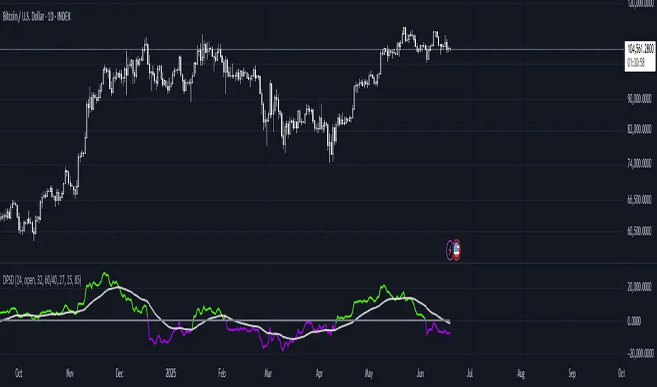
Deviation Adjusted MA Overview
The Deviation Adjusted MA is a custom indicator that enhances traditional moving average techniques by introducing a volatility-based adjustment. This adjustment is implemented by incorporating the standard deviation of price data, making the moving average more adaptive to market conditions. The key feature is the combination of a customizable moving average (MA) type and the application of deviation percentage to modify its responsiveness. Additionally, a smoothing layer is applied to reduce noise, improving signal clarity.
Key Components
Customizable Moving Averages
The script allows the user to select from four different types of moving averages:
Simple Moving Average (SMA): A basic average of the closing prices over a specified period.
Exponential Moving Average (EMA): Gives more weight to recent prices, making it more responsive to recent price changes.
Weighted Moving Average (WMA): Weights prices differently, favoring more recent ones but in a linear progression.
Volume-Weighted Moving Average (VWMA): Adjusts the average by trading volume, placing more weight on high-volume periods.
Standard Deviation Calculation
The script calculates the standard deviation of the closing prices over the selected maLength period.
Standard deviation measures the dispersion or volatility of price movements, giving a sense of market volatility.
Deviation Percentage and Adjustment
Deviation Percentage is calculated by dividing the standard deviation by the base moving average and multiplying by 100 to express it as a percentage.
The base moving average is adjusted by this deviation percentage, making the indicator responsive to changes in volatility. The result is a more dynamic moving average that adapts to market conditions.
The parameter devMultiplier is available to scale this adjustment, allowing further fine-tuning of sensitivity.
Smoothing the Adjusted Moving Average
After adjusting the moving average based on deviation, the script applies an additional Exponential Moving Average (EMA) with a length defined by the smoothingLength input.
This EMA serves as a smoothing filter to reduce the noise that could arise from the raw adjustments of the moving average. The smoothing makes trend recognition more consistent and removes short-term fluctuations that could otherwise distort the signal.
Use cases
The Deviation Adjusted MA indicator serves as a dynamic alternative to traditional moving averages by adjusting its sensitivity based on volatility. The script offers extensive customization options through the selection of moving average type and the parameters controlling smoothing and deviation adjustments.
By applying these adjustments and smoothing, the script enables users to better track trends and price movements, while providing a visual cue for changes in market sentiment.

RSI Standard Deviation | viResearchRSI Standard Deviation | viResearch
The "RSI Standard Deviation" indicator, developed by viResearch, introduces a new approach to combining the Relative Strength Index (RSI) with a standard deviation measure to offer a more dynamic view of market momentum. By applying standard deviation to the RSI values, this indicator refines the traditional RSI, providing a more precise and adaptive way to measure overbought and oversold conditions. This unique combination allows traders to better understand the underlying volatility in RSI movements, leading to more informed decisions in trending and ranging markets.
Technical Composition and Calculation:
The core of the "RSI Standard Deviation" lies in calculating the RSI based on user-defined input parameters and then applying standard deviation to these RSI values. This method enhances the sensitivity of the RSI, making it more responsive to market volatility.
RSI Calculation:
RSI Length (len): The script computes the Relative Strength Index over a customizable length (default: 21), offering a traditional measure of momentum in the market. The RSI tracks the speed and change of price movements, oscillating between 0 and 100 to indicate overbought and oversold conditions.
Standard Deviation Applied to RSI:
Standard Deviation Length (sdlen): The script calculates the standard deviation of the RSI values over a user-defined period (default: 35). This standard deviation represents the volatility in RSI movements, adding a new layer of analysis to traditional RSI.
Upper (u) and Lower (d) Bands:
The standard deviation values are used to create upper and lower bands around the RSI, offering an adaptive range that expands or contracts based on market volatility. This helps traders identify moments when the market is more likely to reverse or continue its trend.
Trend Identification:
Uptrend (L): The script identifies an uptrend when the RSI moves above the lower band and stays above the midline (50). This indicates that the market is gaining upward momentum, potentially signaling a long position.
Downtrend (S): A downtrend is identified when the RSI moves below 50, suggesting a weakening market and a potential short position.
Features and User Inputs:
The "RSI Standard Deviation" script offers various customization options, enabling traders to tailor it to their specific needs and strategies:
RSI Length: Traders can adjust the length of the RSI calculation to control how quickly the indicator responds to price movements.
Standard Deviation Length: Adjusting the standard deviation length allows users to control the sensitivity of the upper and lower bands, fine-tuning the indicator’s responsiveness to market volatility.
Source Input: The script can be applied to different price sources, offering flexibility in how it calculates RSI and standard deviation values.
Practical Applications:
The "RSI Standard Deviation" indicator is particularly useful in volatile markets, where traditional RSI may produce false signals due to rapid price movements. By adding a standard deviation measure, traders can filter out noise and better identify trends.
Key Uses:
Trend Following: The standard deviation bands provide a clearer view of momentum shifts in the RSI, allowing traders to follow the trend more confidently.
Volatility Assessment: The indicator dynamically adjusts to market volatility, making it easier to assess when the market is overbought or oversold and when a trend reversal is likely.
Signal Confirmation: By comparing the RSI to the adaptive standard deviation bands, traders can confirm signals and avoid false entries during periods of high volatility.
Advantages and Strategic Value:
The "RSI Standard Deviation" offers several advantages:
Enhanced Precision: The combination of RSI and standard deviation results in a more refined momentum indicator that adapts to market conditions.
Noise Reduction: The standard deviation bands help filter out short-term market noise, making it easier to identify significant trend changes.
Dynamic Volatility Awareness: By using standard deviation, the indicator adjusts its bands based on real-time volatility, providing more accurate overbought and oversold signals.
Summary and Usage Tips:
The "RSI Standard Deviation" is a powerful tool for traders looking to enhance their RSI analysis with volatility measures. For optimal performance, traders should experiment with different RSI and standard deviation lengths to suit their trading timeframe and strategy. Whether used to follow trends or confirm momentum signals, the "RSI Standard Deviation" provides a reliable and adaptive solution for modern trading environments.
