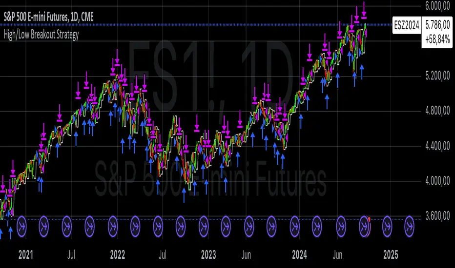
High/Low Breakout Statistical Analysis StrategyThis Pine Script strategy is designed to assist in the statistical analysis of breakout systems on a monthly, weekly, or daily timeframe. It allows the user to select whether to open a long or short position when the price breaks above or below the respective high or low for the chosen timeframe. The user can also define the holding period for each position in terms of bars.
Core Functionality:
Breakout Logic:
The strategy triggers trades based on price crossing over (for long positions) or crossing under (for short positions) the high or low of the selected period (daily, weekly, or monthly).
Timeframe Selection:
A dropdown menu enables the user to switch between the desired timeframe (monthly, weekly, or daily).
Trade Direction:
Another dropdown allows the user to select the type of trade (long or short) depending on whether the breakout occurs at the high or low of the timeframe.
Holding Period:
Once a trade is opened, it is automatically closed after a user-defined number of bars, making it useful for analyzing how breakout signals perform over short-term periods.
This strategy is intended exclusively for research and statistical purposes rather than real-time trading, helping users to assess the behavior of breakouts over different timeframes.
Relevance of Breakout Systems:
Breakout trading systems, where trades are executed when the price moves beyond a significant price level such as the high or low of a given period, have been extensively studied in financial literature for their potential predictive power.
Momentum and Trend Following:
Breakout strategies are a form of momentum-based trading, exploiting the tendency of prices to continue moving in the direction of a strong initial movement after breaching a critical support or resistance level. According to academic research, momentum strategies, including breakouts, can produce returns above average market returns when applied consistently. For example, Jegadeesh and Titman (1993) demonstrated that stocks that performed well in the past 3-12 months continued to outperform in the subsequent months, suggesting that price continuation patterns, like breakouts, hold value .
Market Efficiency Hypothesis:
While the Efficient Market Hypothesis (EMH) posits that markets are generally efficient, and it is difficult to outperform the market through technical strategies, some studies show that in less liquid markets or during specific times of market stress, breakout systems can capitalize on temporary inefficiencies. Taylor (2005) and other researchers have found instances where breakout systems can outperform the market under certain conditions.
Volatility and Breakouts:
Breakouts are often linked to periods of increased volatility, which can generate trading opportunities. Coval and Shumway (2001) found that periods of heightened volatility can make breakouts more significant, increasing the likelihood that price trends will follow the breakout direction. This correlation between volatility and breakout reliability makes it essential to study breakouts across different timeframes to assess their potential profitability .
In summary, this breakout strategy offers an empirical way to study price behavior around key support and resistance levels. It is useful for researchers and traders aiming to statistically evaluate the effectiveness and consistency of breakout signals across different timeframes, contributing to broader research on momentum and market behavior.
References:
Jegadeesh, N., & Titman, S. (1993). Returns to Buying Winners and Selling Losers: Implications for Stock Market Efficiency. Journal of Finance, 48(1), 65-91.
Fama, E. F., & French, K. R. (1996). Multifactor Explanations of Asset Pricing Anomalies. Journal of Finance, 51(1), 55-84.
Taylor, S. J. (2005). Asset Price Dynamics, Volatility, and Prediction. Princeton University Press.
Coval, J. D., & Shumway, T. (2001). Expected Option Returns. Journal of Finance, 56(3), 983-1009.
Gestão de carteira
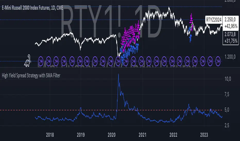
High Yield Spread Strategy with SMA FilterThis Pine Script strategy is designed for statistical analysis and research purposes only, not for live trading or financial decision-making. The script evaluates the relationship between financial volatility (measured by either the VIX or the High Yield Spread) and market positioning strategies (long or short) based on user-defined conditions. Specifically, it allows users to test the assumption that elevated levels of VIX or the High Yield Spread may justify short positions in the market—a widely held belief in financial circles—but this script demonstrates that shorting is not always the optimal choice, even under these conditions.
Key Components:
1. High Yield Spread and VIX:
• High Yield Spread is the difference between the yields of corporate high-yield (or “junk”) bonds and U.S. Treasury securities. A rising spread often reflects increased market risk perception.
• VIX (Volatility Index) is often referred to as the market’s “fear gauge.” Higher VIX levels usually indicate heightened market uncertainty or expected volatility.
2. Strategy Logic:
• The script allows users to specify a threshold for the VIX or High Yield Spread, and it automatically evaluates if the spread exceeds this level, which traditionally would suggest an environment for higher market risk and thus potentially favoring short trades.
• However, the strategy provides flexibility to enter long or short positions, even in a high-risk environment, emphasizing that a high VIX or High Yield Spread does not always warrant shorting.
3. SMA Filter:
• A Simple Moving Average (SMA) filter can be applied to the price data, where positions are only entered if the price is above or below the SMA (depending on the trade direction). This adds a technical component to the strategy, incorporating price trends into decision-making.
4. Hold Duration:
• The script also allows users to define how long to hold a position after entering, enabling an analysis of different timeframes.
Theoretical Background:
The traditional belief that high VIX or High Yield Spreads favor short positions is not universally supported by research. While a spike in the VIX or credit spreads is often associated with increased market risk, research suggests that excessive volatility does not always lead to negative returns. In fact, high volatility can sometimes signal an approaching market rebound.
For example:
• Studies have shown that long-term investments during periods of heightened volatility can yield favorable returns due to mean reversion. Whaley (2000) notes that VIX spikes are often followed by market recoveries as volatility tends to revert to its mean over time .
• Research by Blitz and Vliet (2007) highlights that low-volatility stocks have historically outperformed high-volatility stocks, suggesting that volatility may not always predict negative returns .
• Furthermore, credit spreads can widen in response to broader market stress, but these may overshoot the actual credit risk, presenting opportunities for long positions when spreads are high and risk premiums are mispriced .
Educational Purpose:
The goal of this script is to challenge assumptions about shorting during volatile periods, showing that long positions can be equally, if not more, effective during market stress. By incorporating an SMA filter and customizable logic for entering trades, users can test different hypotheses regarding the effectiveness of both long and short positions under varying market conditions.
Note: This strategy is not intended for live trading and should be used solely for educational and statistical exploration. Misinterpreting financial indicators can lead to incorrect investment decisions, and it is crucial to conduct comprehensive research before trading.
References:
1. Whaley, R. E. (2000). “The Investor Fear Gauge”. The Journal of Portfolio Management, 26(3), 12-17.
2. Blitz, D., & van Vliet, P. (2007). “The Volatility Effect: Lower Risk Without Lower Return”. Journal of Portfolio Management, 34(1), 102-113.
3. Bhamra, H. S., & Kuehn, L. A. (2010). “The Determinants of Credit Spreads: An Empirical Analysis”. Journal of Finance, 65(3), 1041-1072.
This explanation highlights the academic and research-backed foundation of the strategy and the nuances of volatility, while cautioning against the assumption that high VIX or High Yield Spread always calls for shorting.
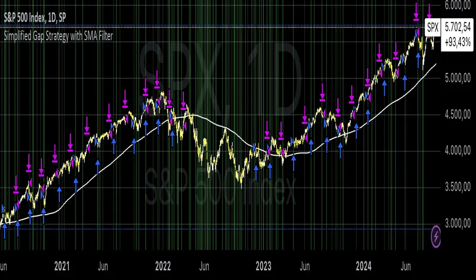
Simplified Gap Strategy with SMA FilterThe Simplified Gap Strategy leverages price gaps as a trading signal, focusing on their significance in market behavior. Gaps occur when the opening price of a security differs significantly from the previous closing price, often signaling potential continuation or reversal patterns.
Key Features:
Gap Threshold:
This strategy requires a minimum percentage gap (defined by the user) to qualify for trading signals.
Directional Trading:
Users can select from various gap types, including "Long Up Gap" and "Short Down Gap," allowing for tailored trading approaches.
SMA Filter:
An optional Simple Moving Average (SMA) filter helps refine trade entries based on trend direction, increasing the probability of successful trades.
Hold Duration:
Positions can be held for a user-defined duration, providing flexibility in trade management.
Statistical Significance of Gaps:
Research has shown that gaps can provide insights into future price movements. According to studies such as those by Hutton and Jiang (2008), price gaps are often followed by momentum in the direction of the gap, indicating that they can serve as reliable indicators for traders. The "Gap Theory" suggests that gaps are filled approximately 90% of the time, emphasizing their relevance in market dynamics (Nikkinen, Sahlström, & Kinnunen, 2006).
Important Note:
This strategy is designed solely for statistical analysis and should not be construed as financial advice. Users are encouraged to conduct their own research and analysis before applying this strategy in live trading scenarios.
By understanding the underlying mechanisms of price gaps and their statistical significance, traders can enhance their decision-making processes and potentially improve trading outcomes.
References:
Hutton, A. W., & Jiang, W. (2008). "Price Gaps: A Guide to Trading Gaps."
Nikkinen, J., Sahlström, P., & Kinnunen, J. (2006). "The Gaps in Financial Markets: An Empirical Study."
This description provides an overview of the strategy while emphasizing its analytical purpose and backing it with relevant academic insights.
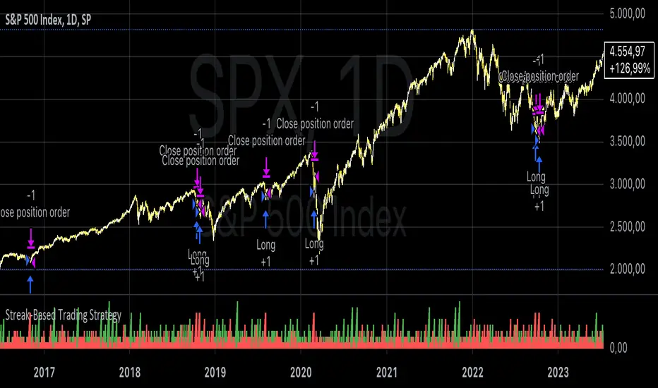
Streak-Based Trading StrategyThe strategy outlined in the provided script is a streak-based trading strategy that focuses on analyzing winning and losing streaks. It’s important to emphasize that this strategy is not intended for actual trading but rather for statistical analysis of streak series.
How the Strategy Works
1. Parameter Definition:
• Trade Direction: Users can choose between “Long” (buy) and “Short” (sell).
• Streak Threshold: Defines how many consecutive wins or losses are needed to trigger a trade.
• Hold Duration: Specifies how many periods the position will be held.
• Doji Threshold: Determines the sensitivity for Doji candles, which indicate market uncertainty.
2. Streak Calculation:
• The script identifies Doji candles and counts winning and losing streaks based on the closing price compared to the previous closing price.
• Streak counting occurs only when no position is currently held.
3. Trade Conditions:
• If the loss streak reaches the defined threshold and the trade direction is “Long,” a buy position is opened.
• If the win streak is met and the trade direction is “Short,” a sell position is opened.
• The position is held for the specified duration.
4. Visualization:
• Winning and losing streaks are plotted as histograms to facilitate analysis.
Scientific Basis
The concept of analyzing streaks in financial markets is well-documented in behavioral economics and finance. Studies have shown that markets often exhibit momentum and trend-following behavior, meaning the likelihood of consecutive winning or losing periods can be higher than what random statistics would suggest (see, for example, “The Behavior of Stock-Market Prices” by Eugene Fama).
Additionally, empirical research indicates that investors often make decisions based on psychological factors influenced by streaks. This can lead to irrational behavior, as they may focus on past wins or losses (see “Behavioral Finance: Psychology, Decision-Making, and Markets” by R. M. F. F. Thaler).
Overall, this strategy serves as a tool for statistical analysis of streak series, providing deeper insights into market behavior and trends rather than being directly used for trading decisions.
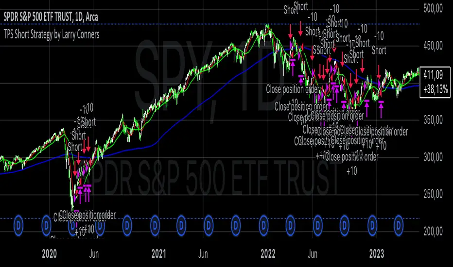
TPS Short Strategy by Larry ConnersThe TPS Short strategy aims to capitalize on extreme overbought conditions in an ETF by employing a scaling-in approach when certain technical indicators signal potential reversals. The strategy is designed to short the ETF when it is deemed overextended, based on the Relative Strength Index (RSI) and moving averages.
Components:
200-Day Simple Moving Average (SMA):
Purpose: Acts as a long-term trend filter. The ETF must be below its 200-day SMA to be eligible for shorting.
Rationale: The 200-day SMA is widely used to gauge the long-term trend of a security. When the price is below this moving average, it is often considered to be in a downtrend (Tushar S. Chande & Stanley Kroll, "The New Technical Trader: Boost Your Profit by Plugging Into the Latest Indicators").
2-Period RSI:
Purpose: Measures the speed and change of price movements to identify overbought conditions.
Criteria: Short 10% of the position when the 2-period RSI is above 75 for two consecutive days.
Rationale: A high RSI value (above 75) indicates that the ETF may be overbought, which could precede a price reversal (J. Welles Wilder, "New Concepts in Technical Trading Systems").
Scaling-In Mechanism:
Purpose: Gradually increase the short position as the ETF price rises beyond previous entry points.
Scaling Strategy:
20% more when the price is higher than the first entry.
30% more when the price is higher than the second entry.
40% more when the price is higher than the third entry.
Rationale: This incremental approach allows for an increased position size in a worsening trend, potentially increasing profitability if the trend continues to align with the strategy’s premise (Marty Schwartz, "Pit Bull: Lessons from Wall Street's Champion Day Trader").
Exit Conditions:
Criteria: Close all positions when the 2-period RSI drops below 30 or the 10-day SMA crosses above the 30-day SMA.
Rationale: A low RSI value (below 30) suggests that the ETF may be oversold and could be poised for a rebound, while the SMA crossover indicates a potential change in the trend (Martin J. Pring, "Technical Analysis Explained").
Risks and Considerations:
Market Risk:
The strategy assumes that the ETF will continue to decline once shorted. However, markets can be unpredictable, and price movements might not align with the strategy's expectations, especially in a volatile market (Nassim Nicholas Taleb, "The Black Swan: The Impact of the Highly Improbable").
Scaling Risks:
Scaling into a position as the price increases may increase exposure to adverse price movements. This method can amplify losses if the market moves against the position significantly before any reversal occurs.
Liquidity Risk:
Depending on the ETF’s liquidity, executing large trades in increments might affect the price and increase trading costs. It is crucial to ensure that the ETF has sufficient liquidity to handle large trades without significant slippage (James Altucher, "Trade Like a Hedge Fund").
Execution Risk:
The strategy relies on timely execution of trades based on specific conditions. Delays or errors in order execution can impact performance, especially in fast-moving markets.
Technical Indicator Limitations:
Technical indicators like RSI and SMA are based on historical data and may not always predict future price movements accurately. They can sometimes produce false signals, leading to potential losses if used in isolation (John Murphy, "Technical Analysis of the Financial Markets").
Conclusion
The TPS Short strategy utilizes a combination of long-term trend filtering, overbought conditions, and incremental shorting to potentially profit from price reversals. While the strategy has a structured approach and leverages well-known technical indicators, it is essential to be aware of the inherent risks, including market volatility, liquidity issues, and potential limitations of technical indicators. As with any trading strategy, thorough backtesting and risk management are crucial to its successful implementation.
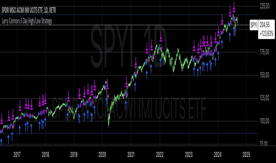
Larry Connors 3 Day High/Low StrategyThe Larry Connors 3 Day High/Low Strategy is a short-term mean-reversion trading strategy that is designed to identify potential buying opportunities when a security is oversold. This strategy is based on the principles developed by Larry Connors, a well-known trading system developer and author.
Key Strategy Elements:
1. Trend Confirmation: The strategy first confirms that the security is in a long-term uptrend by ensuring that the closing price is above the 200-day moving average (condition1). This rule helps filter trades to align with the longer-term trend.
2. Short-Term Pullback: The strategy looks for a short-term pullback by ensuring that the closing price is below the 5-day moving average (condition2). This identifies potential entry points when the price temporarily moves against the longer-term trend.
3. Three Consecutive Lower Highs and Lows:
• The high and low two days ago are lower than those of the day before (condition3).
• The high and low yesterday are lower than those of two days ago (condition4).
• Today’s high and low are lower than yesterday’s (condition5).
These conditions are used to identify a sequence of declining highs and lows, signaling a short-term pullback or oversold condition in the context of an overall uptrend.
4. Entry and Exit Signals:
• Buy Signal: A buy order is triggered when all the above conditions are met (buyCondition).
• Sell Signal: A sell order is executed when the closing price is above the 5-day moving average (sellCondition), indicating that the pullback might be ending.
Risks of the Strategy
1. Mean Reversion Failure: This strategy relies on the assumption that prices will revert to the mean after a short-term pullback. In strong downtrends or during market crashes, prices may continue to decline, leading to significant losses.
2. Whipsaws and False Signals: The strategy may generate false signals, especially in choppy or sideways markets where the price does not follow a clear trend. This can lead to frequent small losses that can add up over time.
3. Dependence on Historical Patterns: The strategy is based on historical price patterns, which do not always predict future price movements accurately. Sudden market news or economic changes can disrupt the pattern.
4. Lack of Risk Management: The strategy as written does not include stop losses or position sizing rules, which can expose traders to larger-than-expected losses if conditions change rapidly.
About Larry Connors
Larry Connors is a renowned trader, author, and founder of Connors Research and TradingMarkets.com. He is widely recognized for his development of quantitative trading strategies, especially those focusing on short-term mean reversion techniques. Connors has authored several books on trading, including “Short-Term Trading Strategies That Work” and “Street Smarts,” co-authored with Linda Raschke. His strategies are known for their systematic, rules-based approach and have been widely used by traders and investment professionals.
Connors’ research often emphasizes the importance of trading with the trend, managing risk, and using statistically validated techniques to improve trading outcomes. His work has been influential in the field of quantitative trading, providing accessible strategies for traders at various skill levels.
References
1. Connors, L., & Raschke, L. (1995). Street Smarts: High Probability Short-Term Trading Strategies.
2. Connors, L. (2009). Short-Term Trading Strategies That Work.
3. Fama, E. F., & French, K. R. (1988). Permanent and Temporary Components of Stock Prices. Journal of Political Economy, 96(2), 246-273.
This strategy and its variations are popular among traders looking to capitalize on short-term price movements while aligning with longer-term trends. However, like all trading strategies, it requires rigorous backtesting and risk management to ensure its effectiveness under different market conditions.
Fractal Proximity MA Aligment Scalping StrategyFractal Analysis
Fractals in trading help identify potential reversal points by marking significant price changes. Our strategy calculates a "fractal value" by comparing the current price to recent high and low fractal points. This is done by evaluating the sum of distances from the current closing price to the recent highs and lows. A positive fractal value suggests proximity to recent lows, hinting at upward momentum. Conversely, a negative value indicates closeness to recent highs, signaling potential downward movement.
Moving Averages for Confirmation
We use a series of 20 moving averages ranging from 5 to 100 to confirm trend directions indicated by fractal analysis. An entry signal is considered bullish when shorter-term moving averages are all above a long-term moving average, aligning with a positive fractal value.
Exit Strategy
The strategy employs dynamic stop-loss levels set at various moving averages, allowing for partial exits when the price crosses below specific thresholds. This helps manage the trade by locking in profits gradually. A full exit might be triggered by strong reversal signals suggested by both fractal values and moving average trends.
This open-source strategy is available for the community to test, adapt, and utilize. Your feedback and modifications are welcome as we refine the approach based on collective user experiences.

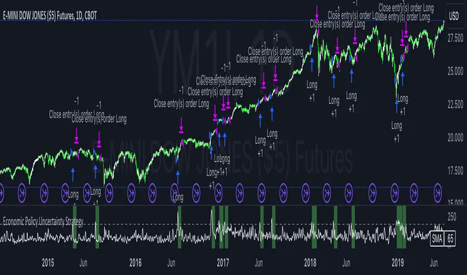
Economic Policy Uncertainty StrategyThis Pine Script strategy is designed to make trading decisions based on the Economic Policy Uncertainty Index for the United States (USEPUINDXD) using a Simple Moving Average (SMA) and a dynamic threshold. The strategy identifies opportunities by entering long positions when the SMA of the Economic Policy Uncertainty Index crosses above a user-defined threshold. An exit is triggered after a set number of bars have passed since the trade was opened. Additionally, the background is highlighted in green when a position is open to visually indicate active trades.
This strategy is intended to be used in portfolio management and trading systems where economic policy uncertainty plays a critical role in decision-making. The index provides insight into macroeconomic conditions, which can affect asset prices and investment returns.
The Economic Policy Uncertainty (EPU) Index is a significant metric used to gauge uncertainty related to economic policies in the United States. This index reflects the frequency of newspaper articles discussing economic uncertainty, government policies, and their potential impact on the economy. It has become a popular indicator for both academics and practitioners to analyze the effects of policy uncertainty on various economic and financial outcomes.
Importance of the EPU Index for Portfolio Decisions:
Economic Policy Uncertainty and Investment Decisions:
Research by Baker, Bloom, and Davis (2016) introduced the Economic Policy Uncertainty Index and explored how increased uncertainty leads to delays in investment and hiring decisions. Their study shows that heightened uncertainty, as captured by the EPU index, is associated with a contraction in economic activity and lower stock market returns. Investors tend to shift their portfolios towards safer assets during periods of high policy uncertainty .
Impact on Asset Prices:
Gulen and Ion (2016) demonstrated that policy uncertainty adversely affects corporate investment, leading to lower stock market returns. The study emphasized that firms reduce investment during periods of high policy uncertainty, which can significantly impact the pricing of risky assets. Consequently, portfolio managers need to account for policy uncertainty when making asset allocation decisions .
Global Implications:
Policy uncertainty is not only a domestic issue. Brogaard and Detzel (2015) found that U.S. economic policy uncertainty has significant spillover effects on global financial markets, affecting equity returns, bond yields, and foreign exchange rates. This suggests that global investors should incorporate U.S. policy uncertainty into their risk management strategies .
These studies underscore the importance of the Economic Policy Uncertainty Index as a tool for understanding macroeconomic risks and making informed portfolio management decisions. Strategies that incorporate the EPU index, such as the one described above, can help investors navigate periods of uncertainty by adjusting their exposure to different asset classes based on economic conditions.
Monthly Purchase Strategy with Dynamic Contract Size This trading strategy is designed to automate monthly purchases of a security, adjusting the size of each purchase based on the percentage of the portfolio's equity. The key features of this strategy include:
Monthly Purchases: The strategy buys the security on a specified day of each month, based on the user's input.
Dynamic Position Sizing: The size of each purchase is calculated as a percentage of the current equity. This allows the position size to adjust dynamically with the portfolio's performance.
Slippage and Commission Considerations: Slippage is simulated by adjusting the entry price by a set number of ticks, while commissions are factored in as fixed costs per trade.
Drawdown Calculation: The strategy tracks the highest equity value and calculates the drawdown, which is the percentage decrease from this peak equity. This helps in assessing the performance and risk of the strategy.
Benefits of the Strategy
Automated Investment: The strategy automates the investment process, reducing the need for manual trading decisions and ensuring consistent execution.
Dynamic Position Sizing: By adjusting the purchase size based on the portfolio’s equity, the strategy helps in managing risk and capitalizing on market movements proportionally to the portfolio’s performance.
Regular Investments: Investing on a regular schedule helps in averaging the purchase price of the security, which can reduce the impact of short-term volatility.
Risk Management: Monitoring drawdown helps in assessing the risk and performance of the strategy, providing insights into potential losses relative to the highest equity value.
Scientific Documentation on ETF Savings Plans
1. Dollar-Cost Averaging and Investment Behavior:
Title: "The Benefits of Dollar-Cost Averaging: A Study of Investment Behavior"
Authors: William F. Sharpe
Journal: Financial Analysts Journal, 1994
Summary: This study discusses the concept of dollar-cost averaging (DCA), which involves investing a fixed amount of money at regular intervals regardless of market conditions. The study highlights that DCA can reduce the impact of market volatility and lower the average cost of investments over time.
Reference: Sharpe, W. F. (1994). The Benefits of Dollar-Cost Averaging: A Study of Investment Behavior. Financial Analysts Journal, 50(4), 27-36.
2. ETFs and Long-Term Investment Strategies:
Title: "Exchange-Traded Funds and Their Role in Long-Term Investment Strategies"
Authors: John C. Bogle
Journal: The Journal of Portfolio Management, 2007
Summary: This paper explores the advantages of using ETFs for long-term investment strategies, emphasizing their low costs, tax efficiency, and diversification benefits. It also discusses how ETFs can be used effectively in automated investment plans like ETF savings plans.
Reference: Bogle, J. C. (2007). Exchange-Traded Funds and Their Role in Long-Term Investment Strategies. The Journal of Portfolio Management, 33(4), 14-25.
3. Risk and Return in ETF Investments:
Title: "Risk and Return Characteristics of Exchange-Traded Funds"
Authors: Eugene F. Fama and Kenneth R. French
Journal: Journal of Financial Economics, 2010
Summary: Fama and French analyze the risk and return characteristics of ETFs compared to traditional mutual funds. The study provides insights into how ETFs can be a viable option for investors seeking diversified exposure while managing risk and optimizing returns.
Reference: Fama, E. F., & French, K. R. (2010). Risk and Return Characteristics of Exchange-Traded Funds. Journal of Financial Economics, 96(2), 257-278.
4. The Impact of Automated Investment Plans:
Title: "The Impact of Automated Investment Plans on Portfolio Performance"
Authors: David G. Blanchflower and Andrew J. Oswald
Journal: Journal of Behavioral Finance, 2012
Summary: This research examines how automated investment plans, including ETF savings plans, affect portfolio performance. It highlights the benefits of automation in reducing behavioral biases and ensuring consistent investment practices.
Reference: Blanchflower, D. G., & Oswald, A. J. (2012). The Impact of Automated Investment Plans on Portfolio Performance. Journal of Behavioral Finance, 13(2), 77-89.
Summary
The "Monthly Purchase Strategy with Dynamic Contract Size and Drawdown" provides a disciplined approach to investing by automating purchases and adjusting position sizes based on portfolio equity. It leverages the benefits of dollar-cost averaging and regular investment, with risk management through drawdown monitoring. Scientific literature supports the effectiveness of ETF savings plans and automated investment strategies in optimizing returns and managing investment risk.

BTC outperform atrategy### Code Description
This Pine Script™ code implements a simple trading strategy based on the relative prices of Bitcoin (BTC) on a weekly and a three-month basis. The script plots the weekly and three-month closing prices of Bitcoin on the chart and generates trading signals based on the comparison of these prices. The code can also be applied to Ethereum (ETH) with similar effectiveness.
### Explanation
1. **Inputs and Variables**:
- The user selects the trading symbol (default is "BINANCE:BTCUSDT").
- `weeklyPrice` retrieves the closing price of the selected symbol on a weekly interval.
- `monthlyPrice` retrieves the closing price of the selected symbol on a three-month interval.
2. **Plotting Data**:
- The weekly price is plotted in blue.
- The three-month price is plotted in red.
3. **Trading Conditions**:
- A long position is suggested if the weekly price is greater than the three-month price.
- A short position is suggested if the three-month price is greater than the weekly price.
4. **Strategy Execution**:
- If the long condition is met, the strategy enters a long position.
- If the short condition is met, the strategy enters a short position.
This script works equally well for Ethereum (ETH) by changing the symbol input to "BINANCE:ETHUSDT" or any other desired Ethereum trading pair.

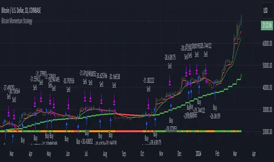
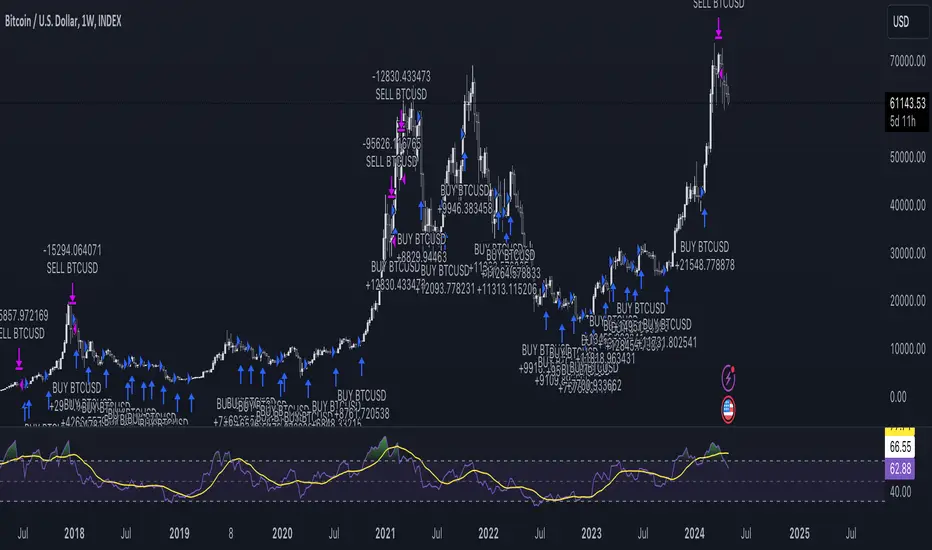
Bitcoin Momentum StrategyThis is a very simple long-only strategy I've used since December 2022 to manage my Bitcoin position.
I'm sharing it as an open-source script for other traders to learn from the code and adapt it to their liking if they find the system concept interesting.
General Overview
Always do your own research and backtesting - this script is not intended to be traded blindly (no script should be) and I've done limited testing on other markets beyond Ethereum and BTC, it's just a template to tweak and play with and make into one's own.
The results shown in the strategy tester are from Bitcoin's inception so as to get a large sample size of trades, and potential returns have diminished significantly as BTC has grown to become a mega cap asset, but the script includes a date filter for backtesting and it has still performed solidly in recent years (speaking from personal experience using it myself - DYOR with the date filter).
The main advantage of this system in my opinion is in limiting the max drawdown significantly versus buy & hodl. Theoretically much better returns can be made by just holding, but that's also a good way to lose 70%+ of your capital in the inevitable bear markets (also speaking from experience).
In saying all of that, the future is fundamentally unknowable and past results in no way guarantee future performance.
System Concept:
Capture as much Bitcoin upside volatility as possible while side-stepping downside volatility as quickly as possible.
The system uses a simple but clever momentum-style trailing stop technique I learned from one of my trading mentors who uses this approach on momentum/trend-following stock market systems.
Basically, the system "ratchets" up the stop-loss to be much tighter during high bearish volatility to protect open profits from downside moves, but loosens the stop loss during sustained bullish momentum to let the position ride.
It is invested most of the time, unless BTC is trading below its 20-week EMA in which case it stays in cash/USDT to avoid holding through bear markets. It only trades one position (no pyramiding) and does not trade short, but can easily be tweaked to do whatever you like if you know what you're doing in Pine.
Default parameters:
HTF: Weekly Chart
EMA: 20-Period
ATR: 5-period
Bar Lookback: 7
Entry Rule #1:
Bitcoin's current price must be trading above its higher-timeframe EMA (Weekly 20 EMA).
Entry Rule #2:
Bitcoin must not be in 'caution' condition (no large bearish volatility swings recently).
Enter at next bar's open if conditions are met and we are not already involved in a trade.
"Caution" Condition:
Defined as true if BTC's recent 7-bar swing high minus current bar's low is > 1.5x ATR, or Daily close < Daily 20-EMA.
Trailing Stop:
Stop is trailed 1 ATR from recent swing high, or 20% of ATR if in caution condition (ie. 0.2 ATR).
Exit on next bar open upon a close below stop loss.
I typically use a limit order to open & exit trades as close to the open price as possible to reduce slippage, but the strategy script uses market orders.
I've never had any issues getting filled on limit orders close to the market price with BTC on the Daily timeframe, but if the exchange has relatively low slippage I've found market orders work fine too without much impact on the results particularly since BTC has consistently remained above $20k and highly liquid.
Cost of Trading:
The script uses no leverage and a default total round-trip commission of 0.3% which is what I pay on my exchange based on their tier structure, but this can vary widely from exchange to exchange and higher commission fees will have a significantly negative impact on realized gains so make sure to always input the correct theoretical commission cost when backtesting any script.
Static slippage is difficult to estimate in the strategy tester given the wide range of prices & liquidity BTC has experienced over the years and it largely depends on position size, I set it to 150 points per buy or sell as BTC is currently very liquid on the exchange I trade and I use limit orders where possible to enter/exit positions as close as possible to the market's open price as it significantly limits my slippage.
But again, this can vary a lot from exchange to exchange (for better or worse) and if BTC volatility is high at the time of execution this can have a negative impact on slippage and therefore real performance, so make sure to adjust it according to your exchange's tendencies.
Tax considerations should also be made based on short-term trade frequency if crypto profits are treated as a CGT event in your region.
Summary:
A simple, but effective and fairly robust system that achieves the goals I set for it.
From my preliminary testing it appears it may also work on altcoins but it might need a bit of tweaking/loosening with the trailing stop distance as the default parameters are designed to work with Bitcoin which obviously behaves very differently to smaller cap assets.
Good luck out there!
DCA StrategyIntroducing the DCA Strategy, a powerful tool for identifying long entry and exit opportunities in uptrending assets like cryptocurrencies, stocks, and gold. This strategy leverages the Heikin Ashi candlestick pattern and the RSI indicator to navigate potential price swings.
Core Functionality:
Buy Signal : A buy signal is generated when a bullish (green) Heikin Ashi candle appears after a bearish (red) one, indicating a potential reversal in a downtrend. Additionally, the RSI must be below a user-defined threshold (default: 85) to prevent buying overbought assets.
Sell Signal : The strategy exits the trade when the RSI surpasses the user-defined exit level (default: 85), suggesting the asset might be overbought.
Backtesting Flexibility : Users can customize the backtesting period by specifying the start and end years.
Key Advantages:
Trend-Following: Designed specifically for uptrending assets, aiming to capture profitable price movements.
Dynamic RSI Integration: The RSI indicator helps refine entry signals by avoiding overbought situations.
User-Defined Parameters: Allows customization of exit thresholds and backtesting periods to suit individual trading preferences.
Commission and Slippage: The script factors in realistic commission fees (0.1%) and slippage (2%) for a more accurate backtesting experience.
Beats Buy-and-Hold: Backtesting suggests this strategy outperforms a simple buy-and-hold approach in uptrending markets.
Overall, the DCA Strategy offers a valuable approach for traders seeking to capitalize on long opportunities in trending markets with the help of Heikin Ashi candles and RSI confirmation.
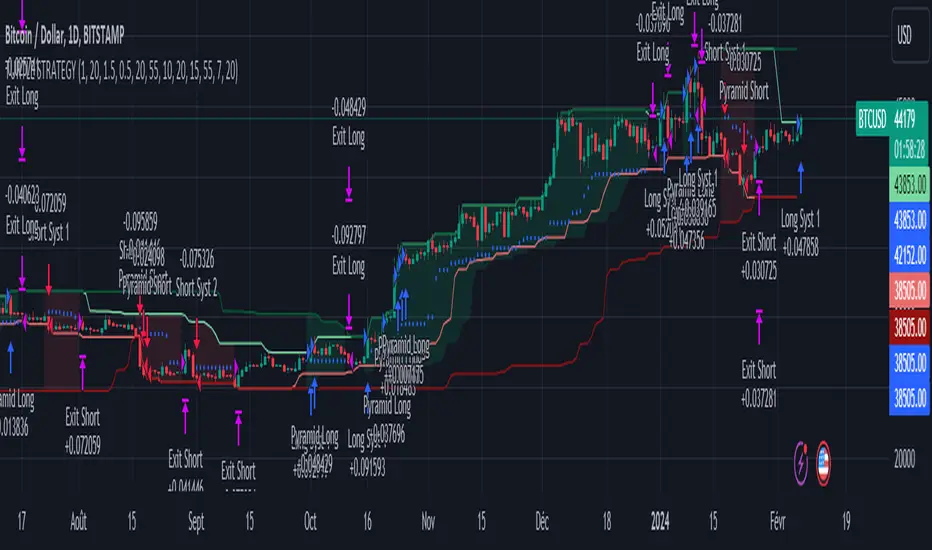
Turtle Trader StrategyTurtle Trader Strategy :
Introduction :
This strategy is based on the well known « Turtle Trader Strategy », that has proven itself over the years. It sends long and short signals with pyramid orders of up to 5, meaning that the strategy can trigger up to 5 orders in the same direction. Good risk and money management.
It's important to note that the strategy combines 2 systems working together (S1 and S2). Let’s describe the specific features of this strategy.
1/ Position size :
Position size is very important for turtle traders to manage risk properly. This position sizing strategy adapts to market volatility and to account (gains and losses). It’s based on ATR (Average True Range) which can also be called « N ». Its length is per default 20.
ATR(20) = (previous_atr(20)*19 + actual_true_range)/20
The number of units to buy is :
Unit = 1% * account/(ATR(20)*dollar_per_point)
where account is the actual account value and dollar_per_point is the variation in dollar of the asset with a 1 point move.
Depending on your risk aversion, you can increase the percentage of your account, but turtle traders default to 1%. If you trade contracts, units must be rounded down by default.
There is also an additional rule to reduce the risk if the value of the account falls below the initial capital : in this case and only in this case, account in the unit formula must be replace by :
account = actual_account*actual_account/initial capital
2/ Open a position :
2 systems are working together :
System 1 : Entering a new 20 day breakout
System 2 : Entering a new 55 day breakout
A breakout is a new high or new low. If it’s a new high, we open long position and vice versa if it’s a new low we enter in short position.
We add an additional rule :
System 1 : Breakout is ignored if last long/short position was a winner
System 2 : All signals are taken
This additional rule allows the trader to be in the major trends if the system 1 signal has been skipped. If a signal for system 1 has been skipped, and next candle is also a new 20 day breakout, S1 doesn’t give a signal. We have to wait S2 signal or wait for a candle that doesn’t make a new breakout to reactivate S1.
3/ Pyramid orders :
Turtle Strategy allows us to add extra units to the position if the price moves in our favor. I've configured the strategy to allow up to 5 orders to be added in the same direction. So if the price varies from 0.5*ATR(20) , we add units with the position size formula. Note that the value of account will be replaced by "remaining_account", i.e. the cash remaining in our account after subtracting the value of open positions.
4/ Stop Loss :
We set a stop loss at 1.5*ATR(20) below the entry price for longs and above the entry price for shorts. If pyramid units are added, the stop is increased/decreased by 0.5*ATR(20). Note that if SL is configured for a loss of more than 10%, we set the SL to 10% for the first entry order to avoid big losses. This configuration does not work for pyramid orders as SL moves by 0.5*ATR(20).
5/ Exit signals :
System 1 :
Exit long on a 10 day low
Exit short on a 10 day high
System 2 :
Exit long on a 20 day low
Exit short on a 20 day high
6/ What types of orders are placed ?
To enter in a position, stop orders are placed meaning that we place orders that will be automatically triggered by the signal at the exact breakout price. Stop loss and exit signals are also stop orders. Pyramid orders are market orders which will be triggered at the opening of the next candle to avoid repainting.
PARAMETERS :
Risk % of capital : Percentage used in the position size formula. Default is 1%
ATR period : ATR length used to calculate ATR. Default is 20
Stop ATR : Parameters used to fix stop loss. Default is 1.5 meaning that stop loss will be set at : buy_price - 1.5*ATR(20) for long and buy_price + 1.5*ATR(20) for short. Turtle traders default is 2 but 1.5 is better for cryptocurrency as there is a huge volatility.
S1 Long : System 1 breakout length for long. Default is 20
S2 Long : System 2 breakout length for long. Default is 55
S1 Long Exit : System 1 breakout length to exit long. Default is 10
S2 Long Exit : System 2 breakout length to exit long. Default is 20
S1 Short : System 1 breakout length for short. Default is 15
S2 Short : System 2 breakout length for short. Default is 55
S1 Short Exit : System 1 breakout length to exit short. Default is 7
S2 Short Exit : System 2 breakout length to exit short. Default is 20
Initial capital : $1000
Fees : Interactive Broker fees apply to this strategy. They are set at 0.18% of the trade value.
Slippage : 3 ticks or $0.03 per trade. Corresponds to the latency time between the moment the signal is received and the moment the order is executed by the broker.
Pyramiding : Number of orders that can be passed in the same direction. Default is 5.
Important : Turtle traders don't trade crypto. For this specific asset type, I modify some parameters such as SL and Short S1 in order to maximize return while limiting drawdown. This strategy is the most optimal on BINANCE:BTCUSD in 1D timeframe with the parameters set per default. If you want to use this strategy for a different crypto please adapt parameters.
NOTE :
It's important to note that the first entry order (long or short) will be the largest. Subsequent pyramid orders will have fewer units than the first order. We've set a maximum SL for the first order of 10%, meaning that you won't lose more than 10% of the value of your first order. However, it is possible to lose more on your pyramid orders, as the SL is increased/decreased by 0.5*ATR(20), which does not secure a loss of more than 10% on your pyramid orders. The risk remains well managed because the value of these orders is less than the value of the first order. Remain vigilant to this small detail and adjust your risk according to your risk aversion.
Enjoy the strategy and don’t forget to take the trade :)
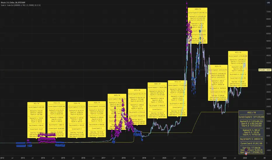
Scale In : Scale OutScale In : Scale Out strategy is an adaptation and extension of dollar-cost-averaging.
As the name implies it not only scales in - allocates a given percentage of available capital to buy at each bar - it also scales out - sells a given percentage of holdings at each bar when a target profit level is reached.
The strategy can potentially mitigate risks associated with market timing.
Although dollar-cost-averaging is often recommended as a strategy for building a position, the management of taking and retaining profits is not often addressed. This strategy demonstrates the potential benefits of managing both the building and (full or partial) liquidation of an investment.
We do not provide any mechanism for managing stop losses. We assume a scale in/out strategy will typically be applied to investing in assets with a high conviction thesis based on criteria external to the strategy. If the strategy does not perform, then the thesis may need to be re-evaluated, and the position liquidated. Even in this case, scaling out should still be considered.
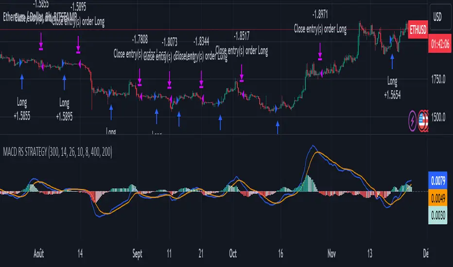
MACD of Relative Strenght StrategyMACD Relative Strenght Strategy :
INTRODUCTION :
This strategy is based on two well-known indicators: MACD and Relative Strenght (RS). By coupling them, we obtain powerful buy signals. In fact, the special feature of this strategy is that it creates an indicator from an indicator. Thus, we construct a MACD whose source is the value of the RS. The strategy only takes buy signals, ignoring SHORT signals as they are mostly losers. There's also a money management method enabling us to reinvest part of the profits or reduce the size of orders in the event of substantial losses.
RELATIVE STRENGHT :
RS is an indicator that measures the anomaly between momentum and the assumption of market efficiency. It is used by professionals and is one of the most robust indicators. The idea is to own assets that do better than average, based on their past performance. We calculate RS using this formula :
RS = close/highest_high(RS_Length)
Where highest_high(RS_Length) = highest value of the high over a user-defined time period (which is the RS_Length).
We can thus situate the current price in relation to its highest price over this user-defined period.
MACD (Moving Average Convergence - Divergence) :
This is one of the best-known indicators, measuring the distance between two exponential moving averages : one fast and one slower. A wide distance indicates fast momentum and vice versa. We'll plot the value of this distance and call this line macdline. The MACD uses a third moving average with a lower period than the first two. This last moving average will give a signal when it crosses the macdline. It is therefore constructed using the values of the macdline as its source.
It's important to note that the first two MAs are constructed using RS values as their source. So we've just built an indicator of an indicator. This kind of method is very powerful because it is rarely used and brings value to the strategy.
PARAMETERS :
RS Length : Relative Strength length i.e. the number of candles back to find the highest high and compare the current price with this high. Default is 300.
MACD Fast Length : Relative Strength fast EMA length used to plot the MACD. Default is 14.
MACD Slow Length : Relative Strength slow EMA length used to plot the MACD. Default is 26.
MACD Signal Smoothing : Macdline SMA length used to plot the MACD. Default is 10.
Max risk per trade (in %) : The maximum loss a trade can incur (in percentage of the trade value). Default is 8%.
Fixed Ratio : This is the amount of gain or loss at which the order quantity is changed. Default is 400, meaning that for each $400 gain or loss, the order size is increased or decreased by a user-selected amount.
Increasing Order Amount : This is the amount to be added to or subtracted from orders when the fixed ratio is reached. The default is $200, which means that for every $400 gain, $200 is reinvested in the strategy. On the other hand, for every $400 loss, the order size is reduced by $200.
Initial capital : $1000
Fees : Interactive Broker fees apply to this strategy. They are set at 0.18% of the trade value.
Slippage : 3 ticks or $0.03 per trade. Corresponds to the latency time between the moment the signal is received and the moment the order is executed by the broker.
Important : A bot has been used to test the different parameters and determine which ones maximize return while limiting drawdown. This strategy is the most optimal on BITSTAMP:ETHUSD in 8h timeframe with the parameters set by default.
ENTER RULES :
The entry rules are very simple : we open a long position when the MACD value turns positive. You are therefore LONG when the MACD is green.
EXIT RULES :
We exit a position (whether losing or winning) when the MACD becomes negative, i.e. turns red.
RISK MANAGEMENT :
This strategy can incur losses, so it's important to manage our risks well. If the position is losing and has incurred a loss of -8%, our stop loss is activated to limit losses.
MONEY MANAGEMENT :
The fixed ratio method was used to manage our gains and losses. For each gain of an amount equal to the value of the fixed ratio, we increase the order size by a value defined by the user in the "Increasing order amount" parameter. Similarly, each time we lose an amount equal to the value of the fixed ratio, we decrease the order size by the same user-defined value. This strategy increases both performance and drawdown.
Enjoy the strategy and don't forget to take the trade :)
Rate of Change StrategyRate of Change Strategy :
INTRODUCTION :
This strategy is based on the Rate of Change indicator. It compares the current price with that of a user-defined period of time ago. This makes it easy to spot trends and even speculative bubbles. The strategy is long term and very risky, which is why we've added a Stop Loss. There's also a money management method that allows you to reinvest part of your profits or reduce the size of your orders in the event of substantial losses.
RATE OF CHANGE (ROC) :
As explained above, the ROC is used to situate the current price compared to that of a certain period of time ago. The formula for calculating ROC in relation to the previous year is as follows :
ROC (365) = (close/close (365) - 1) * 100
With this formula we can find out how many percent the change in the current price is compared with 365 days ago, and thus assess the trend.
PARAMETERS :
ROC Length : Length of the ROC to be calculated. The current price is compared with that of the selected length ago.
ROC Bubble Signal : ROC value indicating that we are in a bubble. This value varies enormously depending on the financial product. For example, in the equity market, a bubble exists when ROC = 40, whereas in cryptocurrencies, a bubble exists when ROC = 150.
Stop Loss (in %) : Stop Loss value in percentage. This is the maximum trade value percentage that can be lost in a single trade.
Fixed Ratio : This is the amount of gain or loss at which the order quantity is changed. The default is 400, which means that for each $400 gain or loss, the order size is increased or decreased by an amount chosen by the user.
Increasing Order Amount : This is the amount to be added to or subtracted from orders when the fixed ratio is reached. The default is $200, which means that for every $400 gain, $200 is reinvested in the strategy. On the other hand, for every $400 loss, the order size is reduced by $200.
Initial capital : $1000
Fees : Interactive Broker fees apply to this strategy. They are set at 0.18% of the trade value.
Slippage : 3 ticks or $0.03 per trade. Corresponds to the latency time between the moment the signal is received and the moment the order is executed by the broker.
Important : A bot has been used to test the different parameters and determine which ones maximize return while limiting drawdown. This strategy is the most optimal on BITSTAMP:BTCUSD in 1D timeframe with the following parameters :
ROC Length = 365
ROC Bubble Signal = 180
Stop Loss (in %) = 6
LONG CONDITION :
We are in a LONG position if ROC (365) > 0 for at least two days. This allows us to limit noise and irrelevant signals to ensure that the ROC remains positive.
SHORT CONDITION :
We are in a SHORT position if ROC (365) < 0 for at least two days. We also open a SHORT position when the speculative bubble is about to burst. If ROC (365) > 180, we're in a bubble. If the bubble has been in existence for at least a week and the ROC falls back below this threshold, we can expect the asset to return to reasonable prices, and thus a downward trend. So we're opening a SHORT position to take advantage of this upcoming decline.
EXIT RULES FOR WINNING TRADE :
The strategy is self-regulating. We don't exit a LONG trade until a SHORT signal has arrived, and vice versa. So, to exit a winning position, you have to wait for the entry signal of the opposite position.
RISK MANAGEMENT :
This strategy is very risky, and we can easily end up on the wrong side of the trade. That's why we're going to manage our risk with a Stop Loss, limiting our losses as a percentage of the trade's value. By default, this percentage is set at 6%. Each trade will therefore take a maximum loss of 6%.
If the SL has been triggered, it probably means we were on the wrong side. This is why we change the direction of the trade when a SL is triggered. For example, if we were SHORT and lost 6% of the trade value, the strategy will close this losing trade and open a long position without taking into account the ROC value. This allows us to be in position all the time and not miss the best opportunities.
MONEY MANAGEMENT :
The fixed ratio method was used to manage our gains and losses. For each gain of an amount equal to the value of the fixed ratio, we increase the order size by a value defined by the user in the "Increasing order amount" parameter. Similarly, each time we lose an amount equal to the value of the fixed ratio, we decrease the order size by the same user-defined value. This strategy increases both performance and drawdown.
NOTE :
Please note that the strategy is backtested from 2017-01-01. As the timeframe is 1D, this strategy is a medium/long-term strategy. That's why only 34 trades were closed. Be careful, as the test sample is small and performance may not necessarily reflect what may happen in the future.
Enjoy the strategy and don't forget to take the trade :)

Narrow Range StrategyNarrow Range Strategy :
INTRODUCTION :
This strategy is based on the Narrow Range Day concept, implying that low volatility will generate higher volatility in the days ahead. The strategy sends us buy and sell signals with well-defined profit targets. It's a medium/long-term strategy. There's also a money management method that allows us to reinvest part of the profits or reduce the size of orders in the event of substantial losses.
NARROW RANGE (NR) DAY :
A Narrow Range Day is a day in which price variations are included in those of a specific day some time before. The high and low of this specific day form the "reference range". In general, we compare these variations with those of 4 or 7 days ago. The mathematical formula for finding an NR4 is :
If low > low(4) and high < high(4) :
nr = true
This implies that the current low is greater than the low of 4 days ago, and the current high is smaller than the high of 4 days ago. So today's volatility is lower than that of 4 days ago, and may be a sign of high volatility to come.
PARAMETERS :
Narrow Range Length : Corresponds to the number of candles back to compare current volatility. The default is 4, allowing comparison of current volatility with that of 4 candles ago.
Stop Loss : Percentage of the reference range on which to set an exit order to limit losses. The minimum value is 0.001, while the maximum is 1. The default value is 0.35.
Fixed Ratio : This is the amount of gain or loss at which the order quantity is changed. The default is 400, which means that for each $400 gain or loss, the order size is increased or decreased by an amount chosen by the user.
Increasing Order Amount : This is the amount to be added to or subtracted from orders when the fixed ratio is reached. The default is $200, which means that for every $400 gain, $200 is reinvested in the strategy. On the other hand, for every $400 loss, the order size is reduced by $200.
Initial capital : $1000
Fees : Interactive Broker fees apply to this strategy. They are set at 0.18% of the trade value.
Slippage : 3 ticks or $0.03 per trade. Corresponds to the latency time between the moment the signal is received and the moment the order is executed by the broker.
Important : A bot was used to test NR4 and NR7 with all possible Stop Losses in order to find out which combination generates the highest return on BITSTAMP:ETHUSD while limiting the drawdown. This strategy is the most optimal with an NR4 and a SL of 35% of the reference range size in 5D timeframe.
BUY AND SHORT SIGNALS :
When an NR is spotted, we create two stop orders on the high and low of the reference range. As soon as there's a breakout from this reference range (shown in blue on the chart), we open a position. We're LONG if there's a breakout on the high and SHORT if there's a breakout on the low. Executing a stop order cancels the second stop order.
RISK MANAGEMENT :
This strategy is subject to losses. We manage our risk with Stop Losses. The user is free to enter a SL as a percentage of the reference range. The maximum amount risked per trade therefore depends on the size of the range. The larger the range, the greater the risk. That's why we have set a maximum Stop Loss to 10% to limiting risks per trade.
The special feature of this strategy is that it targets a precise profit objective. This corresponds to the size of the reference range at the top of the high if you're LONG, or at the bottom of the low if you're short. In the same way, the larger the reference range, the greater the potential profits.
The risk reward remains the same for all trades and amounts to : 100/35 = 2.86. If the reference range is too high, we have set a SL to 10% of the trade value to limit losses. In that case, the risk reward is less than 2.86.
MONEY MANAGEMENT :
The fixed ratio method was used to manage our gains and losses. For each gain of an amount equal to the value of the fixed ratio, we increase the order size by a value defined by the user in the "Increasing order amount" parameter. Similarly, each time we lose an amount equal to the value of the fixed ratio, we decrease the order size by the same user-defined value. This strategy increases both performance and drawdown.
NOTE :
Please note that the strategy is backtested from 2017-01-01. As the timeframe is 5D, this strategy is a medium/long-term strategy. That's why only 37 trades were closed. Be careful, as the test sample is small and performance may not necessarily reflect what may happen in the future.
Enjoy the strategy and don't forget to take the trade :)

2 Moving Averages | Trend FollowingThe trading system is a trend-following strategy based on two moving averages (MA) and Parabolic SAR (PSAR) indicators.
How it works:
The strategy uses two moving averages: a fast MA and a slow MA.
It checks for a bullish trend when the fast MA is above the slow MA and the current price is above the fast MA.
It checks for a bearish trend when the fast MA is below the slow MA and the current price is below the fast MA.
The Parabolic SAR (PSAR) indicator is used for additional trend confirmation.
Long and short positions can be turned on or off based on user input.
The strategy incorporates risk management with stop-loss orders based on the Average True Range (ATR).
Users can filter the backtest date range and display various indicators.
The strategy is designed to work with the date range filter, risk management, and user-defined positions.
Features:
Trend-following strategy.
Two customizable moving averages.
Parabolic SAR for trend confirmation.
User-defined risk management with stop-loss based on ATR.
Backtest date range filter.
Flexibility to enable or disable long and short positions.
This trading system provides a comprehensive approach to trend-following and risk management, making it suitable for traders looking to capture trends with controlled risk.

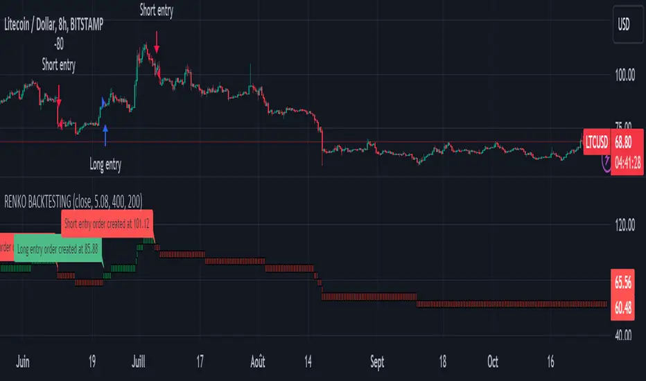
Renko StrategyRENKO STRATEGY
CAUTION : This strategy must be applied to a candlestick chart (not a Renko chart).
INTRODUCTION :
The Traditional Renko chart has been reproduced and is plotted according to the evolution of the price. It will enable us to receive buy or sell signals and follow major trends. This is a medium/long term strategy and depends a lot on the box size chosen in the parameters. There's also a money management method allowing us to reinvest part of the profits or reduce the size of orders in the event of substantial losses.
RENKO CHART :
Renko chart construction methodology :
The user must first choose the box size. The minimum is 0.00001 and there is no maximum. The default is 10. The user must then choose the source that will define the data on which the calculations will be based (high, low, open, close). By default, close is selected. The first candle on the chart is used to draw the first box with its high and low.
Each time the price changes by the amount of the box size relative to the high or low of the last box, a new box is added above or below the previous one. If price variations are less than the box size, the same box is added next to the previous one. If price variations are N (integer number) times greater than box size, N boxes are added above or below the previous one. Each box added above the previous one is a green box, while each box added below the previous one is a red box.
Conditions for drawing a green box above the previous one :
(source - high_of_the_last_box) / box_size > 1
Condition for drawing a red box below the previous one :
(low_of_the_last_box - source) / box_size > 1
If neither condition is triggered, the same box is drawn next to the previous one.
Example :
The last candle has drawn a box with low 12 and high 14. The box size is therefore 2. The strategy will look at the value of the close each time a candle ends. The current candle closes with a close equal to 15.5. As the variation from the previous high is only 1.5 (which is less than the box size), the same box is added next to the previous one. The next candle closes at 16.2. The price variation is therefore 2.2 compared with the previous high. We can now add a new green box just above the previous one, with a low of 14 and a high of 16. The same process applies if the candle's close is at least one box size below the low of the last box. In this case, a new red box is placed below the previous one.
PARAMETERS :
Source : Allows you to specify which data will be taken into account by the strategy when performing calculations. The default is close.
Box size : Size of Renko graph boxes. This is a very important parameter to choose carefully, as it has a strong impact on the strategy's performance. Defaults to 10.
Fixed Ratio : This is the amount of gain or loss at which the order quantity is changed. The default is 400, meaning that for each $400 gain or loss, the order size is increased or decreased by a user-selected amount.
Increasing Order Amount : This is the amount to be added to or subtracted from orders when the fixed ratio is reached. The default is $200, which means that for every $400 gain, $200 is reinvested in the strategy. On the other hand, for every $400 loss, the order size is reduced by $200.
Initial capital : $1000
Fees : Interactive Broker fees apply to this strategy. They are set at 0.18% of the trade value.
Slippage : 3 ticks or $0.03 per trade. Corresponds to the latency time between the moment the signal is received and the moment the order is executed by the broker.
Important : A bot has been used to test all possible box sizes to find out which one generates the highest return on BITSTAMP:LTCUSD while limiting the drawdown. This strategy is the most optimal with a box size equal to 5.08 in 8h timeframe.
BUY AND SHORT SIGNALS :
As the aim of this strategy is to follow major trends based on price movements, we need to be on the right side of price fluctuation. We trade every box reversal, i.e. we are LONG when the boxes are green indicating an uptrend and SHORT when they are red indicating a downtrend.
RISK MANAGEMENT :
This strategy can incur losses. The size of the box is decisive, as it is used to plot the RENKO chart and thus trigger buy or sell signals. It's also what allows us to manage risk. For every trade, we risk a maximum amount equal to 2 times the size of the box, i.e. :(5.08*2*nb_contract)/trade_value.
MONEY MANAGEMENT :
The fixed ratio method has been used to manage our gains and losses. For each gain of an amount equal to the value of the fixed ratio, we increase the order size by a value defined by the user in the "Increasing order amount" parameter. Similarly, each time we lose an amount equal to the value of the fixed ratio, we decrease the order size by the same user-defined value. This strategy not only increases our performance, but also our drawdown.
Enjoy the strategy and don't forget to take the trade :)
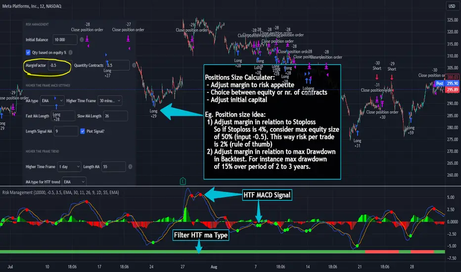
Risk Management and Positionsize - MACD exampleMastering Risk Management
Risk management is the cornerstone of successful trading, and it's often the difference between turning a profit and suffering a loss. In light of its importance, I share a risk management tool which you can use for your trading strategies. The script not only assists in position sizing but also comes with built-in technical features that help in market timing. Let's delve into the nitty-gritty details.
Input Parameter: MarginFactor
One of the key features of the script is the MarginFactor input parameter. This element lets you control the portion of your equity used for placing each trade. A MarginFactor of -0.5 means 50% of your total equity will be deployed in placing the position size. Although Tradingview has a built-in option to adjust position sizing in a same way, I personally prefer to have the logic in my pinecode script. The main reason is userexperience in managing and testing different settings for different charts, timeframes and instruments (with the same strategy).
Stoploss and MarginFactor
If your strategy has a 4% stop-loss, you can choose to use only 50% of your equity by setting the MarginFactor to -0.5. In this case, you are effectively risking only 2% of your total capital per trade, which aligns well with the widely-accepted rule of thumb suggesting a 1-2% risk per trade. Similar if your stoploss is only 1% you can choose to change the MarginFactor to 1, resulting in a positionsize of 200% of your equity. The total risk would be again 2% per trade if your stoploss is set to 1%.
Max Drawdown and MarginFactor
Your MarginFactor setting can also be aligned with the maximum drawdown of your strategy, seen during a backtested period of 2-3 years. For example, if the max drawdown is 15%, you could calibrate your MarginFactor accordingly to limit your risk exposure.
Option to Toggle Number of Contracts
The script offers the option to toggle between using a percentage of equity for position sizing or specifying a fixed number of contracts. Utilizing a percentage of equity might yield unrealistic backtest results, especially over longer periods. This occurs because as the capital grows, the absolute position size also increases, potentially inflating the accumulated returns generated by the backtester. On the other hand, setting a fixed number of contracts as your position size offers a more stable and realistic ROI over the backtested period, as it removes the compounding effect on position sizes.
Key Features Strategy
MACD High Time Frame Entry and Exit Logic
The strategy employs a high time frame MACD (Moving Average Convergence Divergence) to make entry and exit decisions. You can easily adjust the timeframe settings and MACD settings in the inputsection to trade on lower timeframes. For more information on the HTF MACD with dynamic smoothing see:
Moving Average High Time Frame Filter
To reduce market 'noise', the strategy incorporates a high time frame moving average filter. This ensures that the trades are aligned with the dominant market trend (trading the trend). In the inputsection traders can easily switch between different type of moving averages. For more information about this HTF filter see:
Dynamic Smoothing
The script includes a feature for dynamic smoothing. The script contains The timeframeToMinutes(tf) function to convert any given time frame into its equivalent in minutes. For example, a daily (D) time frame is converted into 1440 minutes, a weekly (W) into 10,080 minutes, and so forth. Next the smoothing factor is calculated by dividing the minutes of the higher time frame by those of the current time frame. Finally, the script applies a Simple Moving Average (SMA) over the MACD, SIGNAL, and HIST values, MA filter using the dynamically calculated smoothing factor.
User Convenience: One of the major benefits is that traders don't need to manually adjust the smoothing factor when switching between different time frames. The script does this dynamically.
Visual Consistency: Dynamic smoothing helps traders to more accurately visualize and interpret HTF indicators when trading on lower time frames.
Time Frame Restriction: It's crucial to note that the operational time frame should always be lower than the time frame selected in the input sections for dynamic smoothing to function as intended.
By incorporating this dynamic smoothing logic, the script offers traders a nuanced yet straightforward way to adapt High Time Frame indicators for lower time frame trading, enhancing both adaptability and user experience.
Limitations: Exit Strategy
It's crucial to note that the script comes with a simplified exit strategy, devoid of features like a stop-loss, trailing stop-loss or multiple take profits. This means that while the script focuses on entries and risk management, it might result in higher losses if market conditions unexpectedly turn unfavorable.
Conclusion
Effective risk management is pivotal for trading success, and this TradingView script is designed to give you a better idea how to implement positions sizing with your preferred strategy. However, it's essential to note that this tool should not be considered financial advice. Always perform your due diligence and consult with financial advisors before making any trading decisions.
Feel free to use this risk management tool as building block in your trading scripts, Happy Trading!
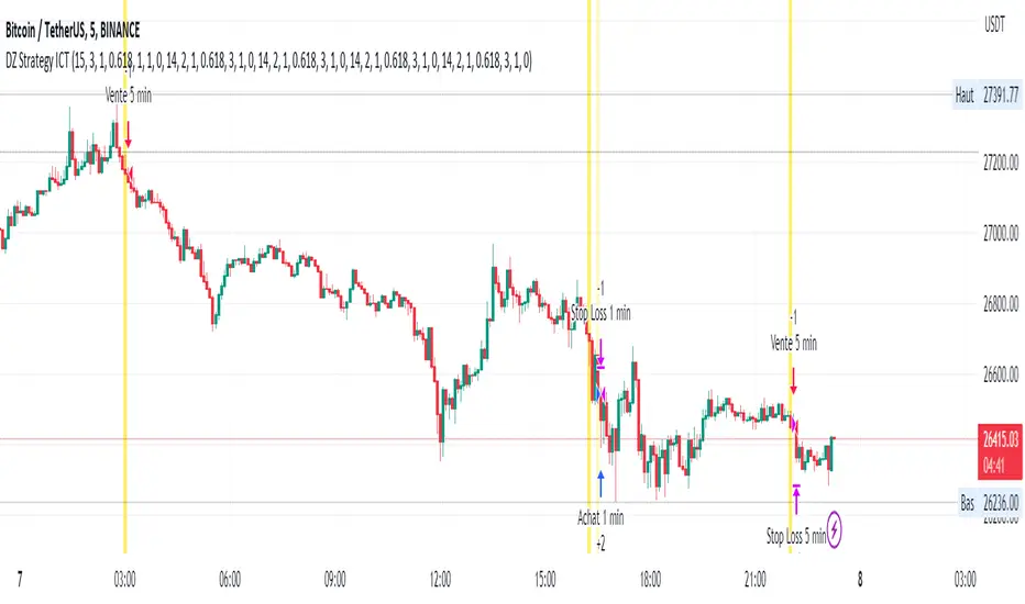
DZ Strategy ICTThe script presented is a trading strategy called "Breaker Block Strategy with Price Channel". This strategy uses multiple time frames (1 minute, 5 minutes, 15 minutes, 1 hour, and 4 hours) to detect support and resistance areas on the chart.
The strategy uses parameters such as length, deviations, multiplier, Fibonacci level, move lag and volume threshold for each time frame. These parameters are adjustable by the user.
The script then calculates support and resistance levels using the simple moving average (SMA) and standard deviation (STDEV) of closing prices for each time frame.
It also detects "Breaker Blocks" based on price movement from support and resistance levels, as well as trade volume. A Breaker Block occurs when there is a significant breakout of a support or resistance level with high volume.
Buy and sell signals are generated based on the presence of a Breaker Block and price movement from support and resistance levels. When a buy signal is generated, a buy order is placed, and when a sell signal is generated, a sell order is placed.
The script also plots price channels for each time frame, representing resistance and support levels.
Profit limit levels are set for each time range, indicating that the price levels assigned to positions should be closed with a profit. Stop-loss levels are also set to limit losses in the event of canceled price movements.
In summary, this trading strategy uses a combination of Breaker Block detection, support and resistance levels, price channels and profit limit levels to generate buy and sell signals and manage positions on different time ranges.
Risk Reward Calculator [lovealgotrading]
OVERVIEW:
This Risk Reward Calculator strategy can help you maximize your RR value with help of algorithmic trading.
INDICATOR:
I wanted to setup my trades more easier with this indicator, I didn't want to calculate everytime before orders, with help this indicator we can calculate R:R value, avarage price, stoploss price, take-profit price, order prices, all position cost and more ...
Our strategy is a risk revard calculation indicator that is made easy to use by using visualized lines and panels, and also has algorithmic trading support.
With the help of this indicator, we can quickly and easily calculate our risk reward values and enter the positions.
If we want to ensure that our balance grows regularly while trading in the stock market, we need to manage the risks and rewards otherwise we may fall below our initial balance at the end of the day, even if we seem to be winning.
What is the Risk-Reward value ?
This value is a value that shows how many times the amount of risk we take when entering the position is successful, we will earn.
- For example, you risked $100 while entering the trade, so if your trade stops, you will lose 100 $.
Your Risk-Reward(RR) value is 2 means that if your position is successful, you will have 200 $ in your pocket.
A trader's success is determined by the amount of R he earns monthly or yearly, not how much money he makes.
What is different in this indicator ?
I want to say thank you to © EvoCrypto. His Calculator (weighted) – evo indicator helped me when I was developed my indicator.
I want to explain what I have improved:
1-In this strategy, we can determine the time period in which we want to open our positions.
2-We can open a maximum of 4 positions in the same direction and close our positions at a single level. StopLoss or TakeProfit
3-This indicator, which works in the form of a strategy, shows where our positions have been opened or closed. With the help of this, it helps us to determine our strategy in our future positions more accurately.
4-The most important improvement is that we do not miss our positions with the help of alarms (WEB HOOK). if we want, we receive by quickly connecting all these positions to our robot, the software can enter and exit the position while we are busy.
IMPLEMENTATION DETAILS – SETTINGS:
1 - We can set the start and end dates of the positions we will take.
2- We can set our take profit, stoploss levels.
3- If your trade is stopped, we can determine the amount of the trade that we will lose.
4- We can adjust our entry levels to positions and our position sizes at entry levels.
(Sum of positions weight must be 100%)
5- We can receive our positions even if we are busy with the help of algorithmic trading. For this, we must paste our Jshon codes into the fields specified in the settings panel.
6- Finally, we can change the settings we want and don't want to have in our visual elements.
Let's make a LONG side example together
We have determined our positions to enter stoploss, take profit and long positions. We did not forget to set the start time of our strategy
Our strategy appear on the graph as follows.
Our strategy has calculated the total position size, our R-R value, the distance of the current price to the stop and take profit levels, in short, a lot of things we could look visually.
Notes:
If you're going to connect this bot to an automatic Long or Short direction,
Don’t forget! you need to Webhook URL,
Don’t miss paste this code to your message window {{strategy.order.alert_message}}
ALSO:
If you have any ideas what to add to my work to add more sources or make calculations cooler, feel free to write me.

Lorentzian Classification Strategy Based in the model of Machine learning: Lorentzian Classification by @jdehorty, you will be able to get into trending moves and get interesting entries in the market with this strategy. I also put some new features for better backtesting results!
Backtesting context: 2022-07-19 to 2023-04-14 of US500 1H by PEPPERSTONE. Commissions: 0.03% for each entry, 0.03% for each exit. Risk per trade: 2.5% of the total account
For this strategy, 3 indicators are used:
Machine learning: Lorentzian Classification by @jdehorty
One Ema of 200 periods for identifying the trend
Supertrend indicator as a filter for some exits
Atr stop loss from Gatherio
Trade conditions:
For longs:
Close price is above 200 Ema
Lorentzian Classification indicates a buying signal
This gives us our long signal. Stop loss will be determined by atr stop loss (white point), break even(blue point) by a risk/reward ratio of 1:1 and take profit of 3:1 where half position will be closed. This will be showed as buy.
The other half will be closed when the model indicates a selling signal or Supertrend indicator gives a bearish signal. This will be showed as cl buy.
For shorts:
Close price is under 200 Ema
Lorentzian Classification indicates a selling signal
This gives us our short signal. Stop loss will be determined by atr stop loss (white point), break even(blue point) by a risk/reward ratio of 1:1 and take profit of 3:1 where half position will be closed. This will be showed as sell.
The other half will be closed when the model indicates a buying signal or Supertrend indicator gives a bullish signal. This will be showed as cl sell.
Risk management
To calculate the amount of the position you will use just a small percent of your initial capital for the strategy and you will use the atr stop loss or last swing for this.
Example: You have 1000 usd and you just want to risk 2,5% of your account, there is a buy signal at price of 4,000 usd. The stop loss price from atr stop loss or last swing is 3,900. You calculate the distance in percent between 4,000 and 3,900. In this case, that distance would be of 2.50%. Then, you calculate your position by this way: (initial or current capital * risk per trade of your account) / (stop loss distance).
Using these values on the formula: (1000*2,5%)/(2,5%) = 1000usd. It means, you have to use 1000 usd for risking 2.5% of your account.
We will use this risk management for applying compound interest.
> In settings, with position amount calculator, you can enter the amount in usd of your account and the amount in percentage for risking per trade of the account. You will see this value in green color in the upper left corner that shows the amount in usd to use for risking the specific percentage of your account.
> You can also choose a fixed amount, so you will have to activate fixed amount in risk management for trades and set the fixed amount for backtesting.
Script functions
Inside of settings, you will find some utilities for display atr stop loss, break evens, positions, signals, indicators, a table of some stats from backtesting, etc.
You will find the settings for risk management at the end of the script if you want to change something or trying new values for other assets for backtesting.
If you want to change the initial capital for backtest the strategy, go to properties, and also enter the commisions of your exchange and slippage for more realistic results.
In risk managment you can find an option called "Use leverage ?", activate this if you want to backtest using leverage, which means that in case of not having enough money for risking the % determined by you of your account using your initial capital, you will use leverage for using the enough amount for risking that % of your acount in a buy position. Otherwise, the amount will be limited by your initial/current capital
I also added a function for backtesting if you had added or withdrawn money frequently:
Adding money: You can choose how often you want to add money (Monthly, yearly, daily or weekly). Then a fixed amount of money and activate or deactivate this function
Withdraw money: You can choose if you want to withdraw a fixed amount or a percentage of earnings. Then you can choose a fixed amount of money, the period of time and activate or deactivate this function. Also, the percentage of earnings if you choosed this option.
Some other assets where strategy has worked
BTCUSD 4H, 1D
ETHUSD 4H, 1D
BNBUSD 4H
SPX 1D
BANKNIFTY 4H, 15 min
Some things to consider
USE UNDER YOUR OWN RISK. PAST RESULTS DO NOT REPRESENT THE FUTURE.
DEPENDING OF % ACCOUNT RISK PER TRADE, YOU COULD REQUIRE LEVERAGE FOR OPEN SOME POSITIONS, SO PLEASE, BE CAREFULL AND USE CORRECTLY THE RISK MANAGEMENT
Do not forget to change commissions and other parameters related with back testing results!. If you have problems loading the script reduce max bars back number in general settings
Strategies for trending markets use to have more looses than wins and it takes a long time to get profits, so do not forget to be patient and consistent !
Please, visit the post from @jdehorty called Machine Learning: Lorentzian Classification for a better understanding of his script!
Any support and boosts will be well received. If you have any question, do not doubt to ask!
