RSI Divergence Strategy BTCRSI Divergence Strategy | Clean
Type: Backtestable strategy
Logic: Uses divergences between price and RSI to generate signals.
LONG: Price makes a lower low, RSI makes a higher low → bullish divergence
SHORT: Price makes a higher high, RSI makes a lower high → bearish divergence
TP / SL: Automatic, based on configurable percentage and Risk/Reward ratio.
Display:
RSI visible in a separate panel
LONG/SHORT signals indicated by small triangles in the RSI panel
Goal: Identify price reversals using relative strength (RSI) and backtest precise trades.
Indicadores e estratégias

ParetoCapital Volatility AlgorithmParetoCapital Volatility Algorithm — Strategy Description
This strategy is a volatility-driven breakout system designed to participate only in markets that exhibit sufficient price activity and structural clarity. All signals are evaluated on candle close to ensure stable, non-repainting behavior.
The strategy adapts its execution logic based on long-term market context while maintaining consistent risk exposure across changing volatility regimes.
Volatility Filter
Trades are taken only when current market volatility exceeds a defined baseline. This filter is intended to suppress signals during low-activity or range-bound conditions and to focus execution on periods where directional movement is more likely to persist.
Market Regime Assessment
A long-term reference is used to classify the prevailing market environment:
When price is positioned above the long-term reference, the market is treated as trend-favorable.
When price is below the reference, the market is treated as non-trend or transitional.
This classification determines how entries are structured but does not attempt to forecast direction.
Entry Logic
In trend-favorable conditions, the strategy seeks continuation trades in the direction of the prevailing trend. Entries are triggered only after price confirms strength through a breakout beyond recent levels.
In non-trend conditions, the strategy prepares for volatility expansion in either direction. Trades are initiated only when price breaks decisively beyond recent boundaries, allowing the market to determine direction.
All entries are confirmation-based and are not executed at market without prior price expansion.
Position Sizing and Risk Control
Position size is dynamically adjusted according to current market volatility. Risk per trade is kept proportional and consistent, while overall capital usage is constrained to prevent overexposure.
This approach allows the strategy to remain risk-controlled during both high- and low-volatility environments.
Exit Logic
Positions are exited when price action indicates a material loss of momentum relative to recent market structure. The exit logic is designed to tolerate minor counter-moves while responding decisively to structural weakness.
Key Characteristics
Candle-close confirmation
Non-repainting behavior
Volatility-adaptive execution
Regime-aware trade logic
Systematic risk management
Strategy Objective
The objective of this strategy is to capture a limited number of structurally strong price movements while minimizing exposure during non-productive market conditions. It prioritizes selectivity, confirmation, and risk discipline over trade frequency.
Usage Notes
The strategy is optimized for major cryptocurrencys, where volatility expansion and momentum continuation are more prevalent.
Best results have been observed on BTCUSD using the 15-minute and 30-minute timeframes.
Performance on other assets or timeframes may vary and should be evaluated through independent testing.

Simple VWMA Smooth | QuantEdgeBSimple VWMA Smooth (SVS) | QuantEdgeB
🔍 What Is Simple VWMA Smooth?
SVS is a smoothed, volume-aware trend filter that blends a Gaussian-pre-filtered, low-lag moving average with dynamic standard-deviation bands. It identifies trends by measuring when price moves decisively above or below a VWMA (Volume-Weighted Moving Average) baseline—filtering out noise while letting high-volume moves carry more influence than low-volume noise.
⚙️ Core Components
1) DEMA Pre-Filter
A double-EMA smoothing step to reduce initial noise before further processing.
2) Gaussian Smoothing
Applies a small-kernel Gaussian filter to produce a cleaner input series that suppresses rapid spikes.
3) VWMA Baseline (Volume-Weighted Average)
Computes a moving average where each bar is weighted by volume, so the baseline tracks “meaningful” price moves more than low-liquidity fluctuations.
• In high volume → the baseline reacts more to those candles
• In low volume → price changes have less impact
4) Volatility Bands
Surrounds the VWMA line with ± N × SD bands (separate multipliers for upper and lower) to capture current market volatility, creating dynamic thresholds for trend detection.
5) Trend Signal
• Long when price closes above the upper band
• Short when price closes below the lower band
• Otherwise neutral
💡 Why It’s Special
• Volume-Validated Responsiveness: VWMA prioritizes moves backed by volume, helping reduce signals caused by thin-market noise.
• Multi-Stage Filtering: The DEMA → Gaussian → VWMA sequence suppresses noise while keeping trend structure clear.
• Asymmetric Bands: Separate multipliers for upper/lower bands let you tune bullish vs bearish sensitivity independently.
• Visual Clarity: Color-coded candles and filled bands highlight trending phases at a glance, while backtest tables quantify performance.
📊 Backtest Mode
SVS includes an optional backtest table, enabling traders to assess historical effectiveness before using it live.
Backtest Metrics Displayed:
• Equity Max Drawdown
• Profit Factor
• Sharpe Ratio
• Sortino Ratio
• Omega Ratio
• Half Kelly
• Total Trades & Win Rate
💼 Ideal Use Cases
• Trend Identification: Spot cleaner trend starts/exits across stocks, FX, or crypto with reduced lag and fewer false breakouts.
• Volume Regimes: Helps distinguish “real” moves (high participation) from weak moves (low participation).
• Multitimeframe Alignment: Confirm direction across timeframes before entries.
• System Building Block: Use as a volume-aware filter inside broader strategies.
🎨 Default Configuration
• DEMA Length: 7
• Gaussian Kernel: length = 4, sigma = 2.0
• VWMA Length: 14
• Volatility Bands: SD length = 40
📌 In Summary
Simple VWMA Smooth | QuantEdgeB is a volume-weighted, noise-suppressed trend filter that combines DEMA smoothing, Gaussian filtering, a VWMA baseline, and dynamic SD bands to separate genuine directional moves from market noise—across any asset or timeframe.
🔹 Disclaimer : Past performance is not indicative of future results. Always backtest and align settings with your risk tolerance and objectives before live trading.
🔹 Strategic Advice : Always backtest, optimize, and align parameters with your trading objectives and risk tolerance before live trading.

RSI Divergence + MTF Table FinalInstitutional RSI Divergence & MTF Confluence Heatmap
Overview
The Institutional RSI Divergence & MTF Confluence Heatmap is a professional-grade analytical tool designed for high-precision traders. It combines Automated RSI Divergence Detection with a Multi-Timeframe (MTF) Heatmap Table, allowing you to monitor market momentum across 8 different timeframes (from 1-minute to 1-day) without ever switching charts.
Key Features
🔍 Automated Divergence Detection: Instantly identifies Regular Bullish and Bearish divergences on the RSI oscillator, marking them with clear "Bull" and "Bear" labels.
📊 MTF Heatmap Grid: A real-time monitoring table that tracks RSI values across: 1m, 5m, 15m, 30m, 1h, 4h, 12h, and 1D.
🎨 Dynamic "Institutional" Color Logic: The table uses a sophisticated color-coded system to highlight extreme exhaustion and momentum:
Ultra Overbought (RSI > 90): Bright Red (Extreme Reversal Zone).
Overbought (RSI > 80): Orange (High Momentum/Caution).
Oversold (RSI < 26): Lime Green (Potential Accumulation).
Neutral: Gray (Consolidation).
🛠️ Flexible Layout Engine: Toggle between Vertical or Horizontal layouts to fit your chart workspace perfectly.
🚀 Pine Script v6 Optimized: Built with the latest TradingView engine for ultra-fast performance and minimal lag.
Trading Strategy: The Power of Confluence
Cross-Timeframe Confirmation: The strongest reversals occur when multiple timeframes (e.g., 15m, 1h, and 4h) all turn Orange/Red or Lime simultaneously. This represents a massive momentum exhaustion.
Divergence Validation: Use the table to see if a detected "Bull" divergence on your current timeframe is backed by "Oversold" conditions on higher timeframes.
Institutional Sniping: Combined with Demand/Supply zones, this script helps you "snipe" entries at the exact moment market momentum peaks or bottoms out.
Settings & Customization
Toggle Compact Mode: Display a minimal version of the table for a cleaner interface.
Custom Thresholds: Modify RSI levels to suit your specific trading style (Scalping vs. Swing Trading).
Table Position: Move the heatmap to any corner of your screen (Top Right, Bottom Left, etc.).
How to Install
Copy the code into your Pine Editor.
Click Save and Add to Chart.
Use the Settings menu to adjust the layout and colors to your preference.
Suggested Tags
#RSI #Divergence #MTF #Heatmap #Institutional #PineScriptV6 #MultiTimeframe

Volume-Based Candle ColoringDisable your Candle Borders, Body and Wicks from the Symbols Settings of your Chart to properly use this Indicator
You can Customize colors and use it to trade as per your Volume preference (Eg. You can turn all the other candles to white if you want to only Trade around breakout of Strong Volume Candles)
Comment Below to request changes
🐍🐢

HS:- HA+BIAS📝 Daily Bias + Heikin Ashi Step Line (Notes)
1️⃣ Indicator Purpose
Combines Daily Market Bias with Heikin Ashi Average
Displays HA average as a STEP LINE WITH BREAKS
HA line changes color based on bias
Works on any timeframe
Bias logic is always calculated from Daily data
2️⃣ Heikin Ashi Calculation
Uses Heikin Ashi candles internally
Does not change chart candles
Formula used:
HA Average = (HA Open + HA Close) / 2
Provides a smoother price reference than normal candles
3️⃣ Daily Reference Levels
Uses previous day:
High
Low
These levels define market structure
Fetched using Daily timeframe regardless of chart timeframe
4️⃣ Positive Bias Condition (Bullish)
Bias becomes POSITIVE only when both conditions are true:
Today Close > Previous Day High
Today Low > Previous Day Low
📌 Indicates strong bullish control
5️⃣ Negative Bias Condition (Bearish)
Bias becomes NEGATIVE only when both conditions are true:
Today Close < Previous Day Low
Today High < Previous Day High
📌 Indicates strong bearish control
6️⃣ Bias Hold Rule (Most Important)
Bias does NOT flip frequently
Bias remains unchanged until:
Both opposite conditions are satisfied
Prevents false signals during sideways markets
Bias Values:
+1 → Positive
-1 → Negative
0 → Neutral
7️⃣ Bias Memory Concept
Bias is stored using a state variable
Previous bias is carried forward when no condition is met
Ensures stable trend direction

kamonosukeThe stop loss is always set at the short-term resistance zone.
If there is no clear resistance level nearby, we zoom out to a higher timeframe and set the target at a key mid-to-long-term level.
Once the setup is complete, we simply wait to see if price moves as expected.
When the target is reached and broken, we take profit and close the trade.

KVS-RSI Target Price- MTF -DivergenceRSI Target Price
MTF
Divergence
KVS-RSI Target Price & Dashboard (MTF) - Divergence
Description: This indicator is a comprehensive Multi-Timeframe (MTF) analysis tool designed to project future price levels based on RSI values. It reverse-engineers the RSI formula to calculate exactly what price is needed for the RSI to hit key levels (Overbought, Oversold, and Pivot).
Key Features:
MTF Support & Resistance: Automatically draws dynamic S/R lines for 4 different timeframes.
Price Projections: Calculates target prices for RSI levels 80, 70, 50 (Pivot), 30, and 20.
Live Dashboard: A customizable table displaying RSI values, projected price targets, and MACD trends for all selected timeframes.

ChoCh Pattern with Trading Levels + Candlestick PatternsBuilt for smart money traders and market structure enthusiasts, the ChoCh Pattern indicator identifies powerful Change of Character reversals with precision. Features intelligent swing point detection, automated risk-reward level plotting, and comprehensive performance tracking to optimize your trading edge in any market condition.
Smart Money Structure Detection - Identifies bullish and bearish Change of Character patterns based market structure analysis and Candlestick patterns Detection,Eliot Waves with T levels
Automated Entry & Exit Levels - Generates entry points with 4 customizable take-profit targets (TP1-TP4) and stop-loss placement based
Real-Time Performance Dashboard - Tracks hit rates for all TP levels, stop-loss statistics, and cumulative P&L across all signals
Visual Trade Management - Clear buy/sell arrows, color-coded level lines, and dynamic price labels for effortless trade execution
Traders seeking systematic risk management with multiple profit targets

KVS-RSI Target Price- MTF RSI Target Price
MTF
Without Divergence
KVS-RSI Target Price & Dashboard (MTF)
Description: This indicator is a comprehensive Multi-Timeframe (MTF) analysis tool designed to project future price levels based on RSI values. It reverse-engineers the RSI formula to calculate exactly what price is needed for the RSI to hit key levels (Overbought, Oversold, and Pivot).
Key Features:
MTF Support & Resistance: Automatically draws dynamic S/R lines for 4 different timeframes.
Price Projections: Calculates target prices for RSI levels 80, 70, 50 (Pivot), 30, and 20.
Live Dashboard: A customizable table displaying RSI values, projected price targets, and MACD trends for all selected timeframes.

All MA Cross StrategyAll MA Cross Strategy is a fully automated, rule-based TradingView strategy built around multiple Moving Average crossovers. It identifies high-probability trend trades while incorporating robust risk management to protect positions and capital.
🔹 Key Features
Supports multiple MA types: SMA, EMA, WMA, HMA, DEMA, TEMA, RMA
Customizable source options: OHLC, HL2, HLC3, OHLC4, Volume
Trend confirmation using ADX and Directional Movement
Optional candle confirmation filter for precise entries
Flexible quantity management (Fixed, Decimal, Exposure)
Compatible with any timeframe or market: Crypto, Forex, Stocks, Indices
🔹 Advanced Risk Management
Stop Loss (Points / % / Pips) to limit potential loss
Target Profit (Points / % / Pips) to secure gains
Multiple Trailing Stop-Loss modes for position protection:
ATR, Adaptive ATR, Dynamic ATR
EMA, SMA, HMA, VWMA
Supertrend, Parabolic SAR, Chandelier Exit
Fractal & Swing High/Low
Profit Factor Adaptive Lock
Automatically chooses the most protective stop (SL or TSL) based on market movement
🔹 Why Protected Technology
The proprietary components that justify the closed-source nature of this strategy lie entirely within its advanced exit engine, which includes protected trailing algorithms, volatility-adaptive structures, and multi-layer risk-shield mechanisms. These functions are the intellectual property of the model and are not present in any open-source variants. The closed-source design ensures that the internal protection logic, trade-survival architecture, and smart-exit sequencing remain secure, tamper-proof, and exclusive to this system.
📈 Smart Trade Management
Automatic position reversal handling
Profit-based dynamic trailing adjustment
Volatility-adaptive ATR calculation
Real-time plotting of entry, SL, TSL & Target
Dashboard displaying live P&L for each position
🧠 Strategy Logic
Long: Fast MA crosses above Slow MA with strong trend confirmation
Short: Fast MA crosses below Slow MA with strong trend confirmation
🔹Default Backtest Logic
This strategy comes pre-configured with realistic and professional default backtest settings:
Initial Capital: $1000
Position Size: 0.01 lots
Commission: 0.05% per trade
Slippage: 5 ticks
Stop Loss / Target: Default off, adjustable
Trailing Stop: Default off, can be enabled via advanced options
MA Lengths: 50/100 EMA (classic trend-following configuration)
Trade Confirmation: Candle confirmation off for simplicity and speed
⚠️ Disclaimer
This strategy is for educational and research purposes only.
It does not constitute financial advice. Always test on paper trading or backtesting before using live. Market conditions vary, and no strategy guarantees profit.

Price By Time - Momentum Flow : Pretty Edition - Aurora BorealisThe Price By Time: Momentum Flow indicator provides a visual representation of market momentum using a colored glow around the price line.
Teal-Green indicates upward (bullish) momentum,
Violet indicates downward (bearish) momentum,
and Pale Blue represents neutral or weak momentum.
The brightness of the glow reflects trend strength, with brighter glows indicating stronger momentum and a likely trend continuation, while fading glows suggest weakening momentum or a potential reversal. Changes in color serve as visual cues for possible trend shifts.
Traders can use this indicator to confirm trend direction, identify optimal entry and exit points, and anticipate changes in momentum, ideally in combination with other technical tools such as support/resistance levels, RSI, or MACD for more robust analysis.

Dragon Flow Arrows (LITE)🚀 DRAGON FLOW ARROWS | Smart Trend Engine + Clean Reversal Arrows
A lightweight but highly-optimized trend system designed for clean charts, powerful visual signals, and no-noise directional flow. Built for traders who want simplicity, clarity, and professional-level momentum-filtered signals without over-complication.
🔥 Dragon Channel (Clean 3-Line Ribbon)
A smooth adaptive channel formed from ATR + EMA, giving you structural trend zones without clutter.
✅ Dragon Flow Gradient
A horizontal, color-shifted flow:
🟢 Bull flow → green glow
🔴 Bear flow → red glow
Automatic blend based on trend direction
Smooth visual transitions (no vertical stripes)
✅ Momentum-Filtered Arrows
BUY/SELL arrows only print when:
Price breaks outside the Dragon Channel
Momentum confirms (RSI + MACD filters)
Trend flips → one clean arrow per direction
✅ Smart Header Panel
At the top of your chart:
📌 Trend: Uptrend / Downtrend / Neutral
⚡ Impulse Strength: Weak / Normal / Strong
📊 How to Use
Entry:
- BUY Setup
Price moving above baseline
Dragon Flow turns bullish (cyan side)
Arrow appears below channel
- SELL Setup
Price breaks below baseline
Dragon Flow turns bearish (magenta side)
Arrow pops above channel
Exit / Filter:
Opposite arrow
Flow color shift
Trend panel flips
Works on Forex, Crypto, Stocks, Indices — all timeframes (just adjust the channel length).
Happy trading!

Trade Secrets by Pratik - Dual Intraday StrategyThe "Trade Secrets by Pratik" strategy is a high-momentum, dual-direction trading system designed to capture explosive moves after brief market pullbacks. It relies on a rigorous combination of trend-following moving averages and a strength filter.
1. Core Concept
The strategy identifies "Clean Pullbacks"—brief pauses in a strong trend where the price stays strictly away from the short-term average (10 EMA). This indicates extreme momentum, as buyers (in an uptrend) or sellers (in a downtrend) are too aggressive to allow a deeper correction.
2. Technical Filters
Trend Direction: Price must be above both 10 and 35 EMAs for Buys, and below both for Sells.
Strength Filter (RSI): Requires an RSI > 60 for Longs (to ensure high demand) and RSI < 40 for Shorts (to ensure heavy selling pressure).
3. Trade Execution
The Setup: Look for a "Floating Candle"—a Red candle for Buys or a Green candle for Sells that does not touch the 10 EMA.
The Trigger: A trade is entered only if the very next candle breaks the "Setup Candle's" high (Buy) or low (Sell).
Risk-Reward: Aim for a fixed 1:3 Ratio, ensuring that one winner covers three losing trades.
4. Safety Logic
The system includes a "No-Same-Candle-Exit" rule, preventing the script from triggering a Stop Loss on the same bar as the Entry. This filters out immediate price "whipsaws" and ensures the trade has room to develop.

DDDDD : EMA Pack (Matched Colors + MTF)📌 DDDDD : EMA Pack (Matched Colors + MTF)
🔹 Concept
DDDDD : EMA Pack is a clean and minimal Exponential Moving Average (EMA) overlay designed for trend structure analysis and multi-timeframe context.
This indicator focuses on visual clarity, consistent color mapping, and optional MTF EMA projection, allowing traders to read market structure without clutter or signal noise.
It is not an entry or signal generator, but a trend and regime visualization tool.
🔹 Logic
The script plots a fixed set of EMAs commonly used to define short-term momentum, intermediate trend, and long-term bias:
EMA 5
EMA 10
EMA 25
EMA 50
EMA 75
EMA 200
Each EMA is calculated using the standard exponential moving average formula.
If a higher timeframe is selected, the EMA is calculated on that timeframe and projected onto the current chart using request.security().
🔹 Methodology
Users may select:
Source price (default: close)
EMA timeframe
Empty = current chart timeframe
Any higher timeframe = true MTF EMA projection
All EMA colors are manually matched and fixed to maintain visual consistency across markets and timeframes.
Line thickness is kept uniform to avoid visual hierarchy bias.
This design ensures the indicator remains purely structural, without repainting logic, smoothing tricks, or adaptive parameters.
🔹 How to Use
Use EMA alignment and spacing to assess:
Trend direction
Trend strength
Compression vs expansion
Higher-timeframe EMA projection can be used as:
Dynamic support/resistance
Trend filter
Regime context for lower-timeframe execution
This indicator works best when combined with:
Price action
Market structure
Separate entry/exit logic of your own system
⚠️ This indicator does not provide buy/sell signals and should not be used alone for trade execution.
🔹 Notes
No repainting beyond standard MTF behavior
No performance or profitability claims
Designed for discretionary and systematic traders
Suitable for stocks, crypto, forex, and indices

ATR 0.5x & 1x Distance (Horizontal)What this version does (no ambiguity)
Plots true horizontal dashed lines
One at ±0.5 × ATR
One at ±1.0 × ATR
Lines extend to the right (proper levels, not floating spaghetti)
ATR is calculated from the active chart timeframe
30m chart → 30m ATR
1H chart → 1H ATR
Clean, stable, no repainting tricks
Important detail (this matters for your strategy)
The lines are anchored to a reference price, which is currently configurable:
Default: close
You can change it to:
VAH
VAL
POC
Any plotted level
This is exactly what you want for:
“How far beyond value has price gone in ATR terms?”
How you’ll likely use this in practice
For your mean-reversion framework:
Anchor Reference Price = VAH or VAL
Treat:
0.5× ATR → probabilistic rejection zone
1.0× ATR → acceptance / thesis failure
No more eyeballing. No more dragging stops because “the candle looked angry.”

RBR / DBR / RBD / DBD Pattern IdentifierThis strategy identifies price-action based continuation and reversal structures using the Rally–Base–Rally (RBR), Drop–Base–Rally (DBR), Rally–Base–Drop (RBD), and Drop–Base–Drop (DBD) patterns.
The logic is based on institutional price behavior, where strong impulsive moves are followed by a low-volatility base (consolidation) and then a confirmation move in the direction of continuation or reversal.
Strong candles represent aggressive participation (demand or supply).
Base candles represent absorption, order balancing, and accumulation/distribution.
Breakout candle confirms intent and directional bias.
Pattern Interpretation
RBR: Bullish continuation after consolidation
DBR: Bullish reversal after selling pressure
RBD: Bearish reversal after buying pressure
DBD: Bearish continuation after consolidation
Usage Guidelines
Best used in alignment with higher-timeframe trend and key supply/demand zones.
Suitable for intraday, swing, and positional trading, with timeframe-specific tuning.
Intended as a structure identification tool, not a standalone trading system.
Risk management, trend context, and confluence with other tools are essential before taking trades.

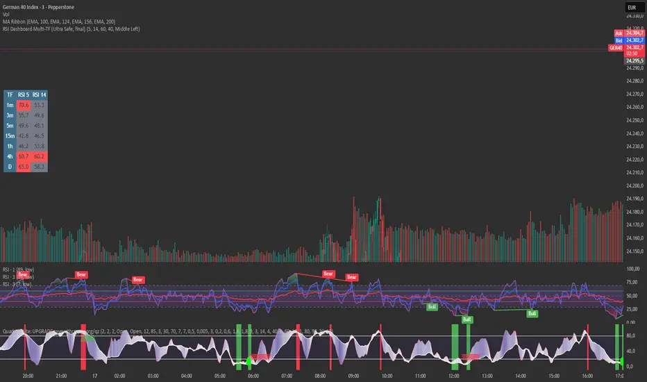
RSI Dashboard Multi-TF This script displays RSI values from multiple timeframes in a compact dashboard directly on the chart.
It is designed for traders who want to quickly identify whether the market is overbought, oversold, or neutral across different timeframes, without constantly switching chart intervals.
The dashboard shows the RSI simultaneously for the following timeframes:
- 1 minute
- 3 minutes
- 5 minutes
- 15 minutes
- 1 hour
- 4 hours
- Daily
Typical use cases:
- Scalping & intraday trading
- Multi-timeframe analysis at a glance
- Entry confirmation (e.g. pullbacks, breakouts)
- Avoiding trades against overbought or oversold market conditions
- Complementing EMA, VWAP, or price action strategies
⚙️ Notes
This dashboard is an analysis tool, not an automated trading system.
No repainting (uses request.security).
Suitable for indices, forex, crypto, and commodities.
This RSI dashboard provides a fast, clear, and visually clean market overview across multiple timeframes, making it an ideal tool for active traders who want to make efficient and well-structured trading decisions.
Delta Volume Bubble [Quant Z-Score] by tncylyvDelta/Volume Bubble by tncylyv
This indicator is a quantitative order flow tool designed to visualize statistically significant volume and delta anomalies directly on the price chart. By moving away from raw, noisy volume numbers and utilizing Z-Score (Standard Score) statistics, this tool adapts to changing market volatility to highlight areas of heavy institutional interest or exhaustion.
It combines statistical analysis with Price Action concepts (Effort vs. Result) to detect "Absorption"—market conditions where high volume occurs with very little price movement.
1. Core Concepts & Methodology
A. Adaptive Z-Score (The "Quant" Logic)
Raw volume data is often difficult to interpret because volume fluctuates wildly between sessions (e.g., the Asian session typically has lower volume than the New York Open).
Instead of using a fixed volume threshold (e.g., "Alert me if volume > 1000"), this script calculates the Z-Score.
It measures how many Standard Deviations (
σ
) the current volume is from the historical average.
Significance: A Z-Score of +2.0 or higher puts the current candle in the top 5% of statistical occurrences, filtering out noise and highlighting true anomalies.
B. Absorption Detection (Effort vs. Result)
This feature identifies "Trapped Traders."
The Logic: If the Z-Score indicates extremely high volume (High Effort), but the price candle has a very small body (Low Result), it implies that aggressive market orders are being absorbed by passive limit orders.
Visual: These specific anomalies can be highlighted with a unique halo effect, signaling a potential reversal or stop-hunt area.
C. Intra-Bar True VWAP (Smart Placement)
Standard indicators usually plot symbols at the High, Low, or Close of a candle.
This script utilizes request.security_lower_tf to analyze the Lower Timeframe (LTF) structure of the specific bar.
It calculates the exact Volume Weighted Average Price (VWAP) of that single candle.
Benefit: The bubble is drawn exactly where the heaviest volume occurred inside the candle, providing a more accurate level for future Support/Resistance tests.
2. Key Features
Dual Data Modes: Switch seamlessly between Volume Delta (Buying vs. Selling pressure) or standard Total Volume.
Dynamic Sizing: Bubble sizes (Small, Medium, Large) scale automatically based on the intensity of the Z-Score.
Absorption Logic: Automatically flags candles where volume is high but price progression is stalled.
Adaptive Visuals: Colors and opacity can fade dynamically based on the strength of the signal, or remain solid based on user preference.
Alert System: Fully configurable alerts for Z-Score breakouts and Absorption detection.
3. How to Use
This tool is best used to identify Reversals and Breakout Validation.
Trend Exhaustion (Climax):
If price is trending up and a large "Bullish" bubble appears at the highs with a long upper wick or small body (Absorption), it may indicate buying exhaustion and passive selling.
Breakout Confirmation:
If price breaks a key support/resistance level accompanied by a Large Bubble (High Z-Score), it confirms institutional backing for the move.
Support/Resistance Defense:
The "True VWAP" location of the bubble often acts as a re-test level. If price retraces to the center of a previous large bubble, observe for a reaction.
4. Settings Guide
Data Settings
Calculation Source: Choose between Volume Delta (Up/Down tick analysis) or Regular Volume.
Lower TF Granularity: The timeframe used to calculate the specific "True VWAP" location inside the bar (e.g., 1S or 1M).
Statistical Lookback: The number of bars used to calculate the baseline Average and Standard Deviation (Default: 60).
Quant Logic
Calculation Mode:
Adaptive (Z-Score): Triggers based on relative statistical anomalies (Recommended).
Fixed: Triggers based on raw volume numbers.
Z-Score Threshold: The sensitivity level. 2.0 is standard; higher values (e.g., 3.0) will show fewer, more extreme signals.
Absorption Logic
Detect Absorption: Enables the calculation for small-bodied high-volume candles.
Absorption Ratio: Defines how "small" the body must be relative to the average to qualify as absorption (0.1 to 1.0).
Visuals
Theme: Switch between Dark (Mint/Coral) and Light (Royal/Sunset) themes.
Scale Size: If enabled, bubbles grow larger as the Z-Score increases.
Glow Effect: Adds a neon glow for better visibility on dark backgrounds.
________________________________________
Risk Disclaimer:
This indicator is for informational and educational purposes only. Volume and Delta analysis are subjective interpretation methods. Past performance, or statistical anomalies shown by this script, do not guarantee future results. Always manage your risk appropriately.

SMC/PA Ultimate V27SMC Ultimate Strategy: Automated Structure & Performance Dashboard
This strategy is designed based on Smart Money Concepts (SMC) principles, utilizing market structure breaks (Zigzag Swings) to identify high-probability reversal setups. It features a fully automated execution engine, dynamic risk management, and a comprehensive real-time performance dashboard.
1. Core Logic & Entry Mechanism
Market Structure: The script uses a Zigzag algorithm (Length = 8 default) to detect significant Swing Highs and Swing Lows.
Entry Trigger:
SHORT: Triggered when the price breaks below the recent Swing Low. The entry order is placed at the 50% Fibonacci retracement of the breakout range.
LONG: Triggered when the price breaks above the recent Swing High. The entry order is placed at the 50% Fibonacci retracement.
Stop Loss (SL): Automatically set at the recent Swing High (for Shorts) or Swing Low (for Longs).
2. Advanced Exit Strategies
Users can choose between two exit modes in the settings:
Fixed Risk:Reward (R:R): Targets a static Reward-to-Risk ratio (e.g., 1:2).
Trailing Stop (%): A dynamic trailing stop that follows price movement (e.g., 3%) to maximize profits during strong trends.
3. Visual Visualization
Red Box: Represents the Risk Zone (Entry to Stop Loss).
Orange/Blue Box: Represents the projected Reward Zone (Entry to TP).
Purple Overlay Box: Appears upon trade closure to show the Realized Profit/Loss Path, giving you a clear visual of how much of the move was captured compared to the theoretical setup.
W/L Labels: Clearly marks trades as W (Win) or L (Loss) on the chart.
4. Professional Risk Management
Integrated position sizing logic inspired by professional capital management:
Position Size: Calculated based on a percentage of Account Equity (Input: Vốn vào lệnh %).
Leverage: Built-in leverage multiplier (Input: Đòn Bẩy x) to simulate futures/margin trading volume.
5. Real-time Monthly Performance Table
A detailed Dashboard located at the bottom-right corner provides instant statistical analysis without needing to open the Strategy Tester panel:
Monthly Breakdown: Displays P/L ($ and %), Winrate, and Win/Loss count for every month in the selected range.
Instant Update: The table updates immediately when a trade closes or on the last bar, ensuring zero lag.
Summary: Shows total Capital used, Leverage, and overall Winrate at the top.
6. Backtest Date Range Filter
Includes a strict date filter (From Year/Month to To Year/Month). The strategy will only execute and calculate statistics within this specific time window, allowing for precise backtesting of specific market conditions.
How to Use
Zigzag Length: Adjust to 5 for scalping or 14+ for swing trading to change sensitivity.
Exit Mode: Select "Trailing Stop %" for trending markets or "Fixed R:R" for ranging markets.
Backtest Range: Ensure the From Year and To Year match the data available on your chart.
Disclaimer: This script is for educational and backtesting purposes only. Past performance does not guarantee future results.

MATRIX AI Trading SystemMATRIX AI Trading System - Complete Trading Guidelines
Core Trading Strategy
Primary Entry Signals (Must Have)
BUY/SELL Arrow Signals - Your main entry trigger
Wait for the green "BUY" arrow (upward triangle) below the candle
Wait for the red "SELL" arrow (downward triangle) above the candle
These are generated by the MATRIX indicator when momentum shifts
AI Score Confirmation
Check the dashboard on the right side
LONG SCORE should be 55+ (preferably 70+) for buy entries
SHORT SCORE should be 55+ (preferably 70+) for sell entries
Green = Strong signal, Yellow/Orange = Moderate, Red = Weak
3-4 Key Confirmations (Use At Least 3)
Confirmation 1: Bollinger Bands (BB) Smooth Area
Best Entry Zones:
For BUY: Price touches or bounces from the lower BB band (blue line at bottom)
For SELL: Price touches or bounces from the upper BB band (blue line at top)
BB Status on Dashboard: Look for "Squeeze" followed by "Expansion" - this indicates volatility breakout
Avoid trading when: Price is in the middle of BB bands with "Normal" status
What to Look For:
Price rejection wicks at BB bands
Candle closes back inside the bands after touching outer band
BB width increasing (expansion phase)
Confirmation 2: RSI Divergence
Check Dashboard Row 9 (RSI):
Bullish Divergence: Look for "Bull Div" label on chart (green label near lows)
Price makes lower low, but RSI makes higher low
Strong reversal signal for BUY trades
Bearish Divergence: Look for "Bear Div" label on chart (red label near highs)
Price makes higher high, but RSI makes lower high
Strong reversal signal for SELL trades
Dashboard Signals:
RSI value shows in green when bullish (<30 zone)
RSI value shows in red when bearish (>70 zone)
"Bull Div" or "Bear Div" text appears in rightmost column
Confirmation 3: Fibonacci Golden Pocket
The Sweet Spot (0.618 - 0.786 retracement):
Yellow shaded zone between two orange lines
Dashboard Row 15 shows: "Inside" or "Outside"
Trading Rules:
BUY Setup: Price pulls back INTO golden pocket, then BUY arrow appears
SELL Setup: Price rallies INTO golden pocket from below, then SELL arrow appears
Best Entries: When price is "Inside" golden pocket + BUY/SELL arrow appears
Trend Continuation: Golden pocket acts as support in uptrends, resistance in downtrends
Confirmation 4: Support & Resistance
Check Dashboard Rows 16-17:
Support Level: Green horizontal line below price
Resistance Level: Red horizontal line above price
Dashboard shows "Near" or "Away"
Trading Rules:
BUY Priority: When dashboard shows "Near" support + BUY arrow
SELL Priority: When dashboard shows "Near" resistance + SELL arrow
Strongest Signals: Multiple touches of S/R level + rejection candles
Wait for confirmation: Don't trade until price clearly respects the level
Additional Power Confirmations
Confirmation 5: Fair Value Gap (FVG)
Visual Identification:
Green semi-transparent boxes = Bullish FVG (price gap up)
Red semi-transparent boxes = Bearish FVG (price gap down)
Small dotted line in the middle of each FVG zone
"FVG" label marks each gap
Trading Strategy:
BUY Setup: Price returns to fill bullish FVG (green box) + BUY arrow
SELL Setup: Price returns to fill bearish FVG (red box) + SELL arrow
Dashboard Row 14: Shows "FVG Up" or "FVG Dn"
FVG zones act as magnets - price often returns to fill them
Confirmation 6: CHoCH (Change of Character)
Structure Break Signals:
Green "CHoCH" label below candle = Bullish structure change
Red "CHoCH" label above candle = Bearish structure change
What It Means:
Market structure has shifted direction
Previous trend is weakening
Potential reversal or new trend beginning
Trading Application:
CHoCH + BUY arrow = Strong bullish reversal setup
CHoCH + SELL arrow = Strong bearish reversal setup
Look for CHoCH near support/resistance for highest probability
Complete Trade Setup Examples
PERFECT BUY SETUP (Use 3-4 Confirmations)
✅ BUY Arrow appears below candle (primary signal)
✅ LONG SCORE 70+ on dashboard (AI confirmation)
✅ Price at lower BB band or bouncing from it (BB confirmation)
✅ "Bull Div" label appears or RSI bullish (divergence confirmation)
✅ "Inside" golden pocket or near 0.618 Fib (Fibonacci confirmation)
✅ "Near" support on dashboard (S/R confirmation)
✅ Bullish FVG zone below or CHoCH green label (SMC confirmation)
Minimum Required: BUY Arrow + 3 of the above confirmations
PERFECT SELL SETUP (Use 3-4 Confirmations)
✅ SELL Arrow appears above candle (primary signal)
✅ SHORT SCORE 70+ on dashboard (AI confirmation)
✅ Price at upper BB band or rejecting from it (BB confirmation)
✅ "Bear Div" label appears or RSI bearish (divergence confirmation)
✅ "Inside" golden pocket or near 0.786 Fib (Fibonacci confirmation)
✅ "Near" resistance on dashboard (S/R confirmation)
✅ Bearish FVG zone above or CHoCH red label (SMC confirmation)
Minimum Required: SELL Arrow + 3 of the above confirmations
Trade Management
Entry Rules:
Wait for confirmation: Arrow + AI Score + minimum 3 confirmations
Best entries: 4+ confirmations aligned = highest probability
Avoid: Trading with only 1-2 confirmations (low probability)
Stop Loss (Automatic on Chart):
Red horizontal line shows your SL level
Based on recent swing high/low (20 periods)
Dashboard shows risk in pips
Take Profit Levels (Automatic on Chart):
TP1 (1:1 R:R): Green dashed line - First profit target
TP2 (2:1 R:R): Green dashed line - Second profit target
TP3 (4:1 R:R): Green solid line - Final profit target
Labels show exact prices, pips, and percentage gains
Position Sizing Strategy:
Close 50% at TP1 (secure profits)
Close 30% at TP2 (let winners run)
Close 20% at TP3 or trail stop (maximum gains)
Dashboard Quick Reference
Top Priority Rows to Check:
Row 1: LONG SCORE (need 55+, prefer 70+)
Row 2: SHORT SCORE (need 55+, prefer 70+)
Row 3-6: TP Hit Rate statistics
Row 8: Trend direction
Row 9: RSI + Divergence status
Row 12: BB status (Squeeze/Expansion/Normal)
Row 14: SMC status (OB/FVG indicators)
Row 15: Fib golden pocket (Inside/Outside)
Row 16-17: S/R proximity (Near/Away)
Row 20: Active trade status
Trading Psychology & Rules
High Probability Setups (Take These):
BUY/SELL arrow + AI Score 70+ + 4 confirmations = STRONG ENTRY
Multiple confluences at same price level = HIGH PROBABILITY
Trend direction + all indicators aligned = BEST TRADES
Low Probability Setups (Skip These):
Arrow appears but AI Score below 45 = WEAK SIGNAL
Only 1-2 confirmations = LOW PROBABILITY
Conflicting signals (bullish and bearish indicators mixed) = STAY OUT
"Sideways" trend + mixed signals = NO TRADE
Golden Rules:
Never trade without the BUY/SELL arrow
Always check AI Score first (must be 55+)
Wait for minimum 3 confirmations
Respect the automatic TP/SL levels
Check TP Hit Rate on dashboard (Row 3-6)
Trade with the trend (Row 8 on dashboard)
Quick Decision Flowchart
STEP 1: Did BUY/SELL arrow appear? → NO = Don't trade / YES = Continue
STEP 2: Is AI Score 55+? → NO = Skip trade / YES = Continue
STEP 3: Count your confirmations:
BB position (at bands?)
RSI Divergence (Bull/Bear Div label?)
Golden Pocket (Inside/Outside?)
S/R Proximity (Near support/resistance?)
FVG zone (price near gap?)
CHoCH label (structure break?)
STEP 4: Do you have 3+ confirmations? → NO = Wait / YES = ENTER TRADE
STEP 5: Set position size and follow automatic TP/SL levels
Success Tips
✅ Patience is key - Wait for all confirmations to align
✅ Quality over quantity - 2-3 high-probability trades better than 10 weak ones
✅ Trust the system - The AI calculates 11 different indicators
✅ Follow TP/SL strictly - They're calculated for optimal risk:reward
✅ Review dashboard - Check TP Hit Rate to see system performance
✅ Trade sessions - Best results during high volume trading hours
✅ Avoid news events - Major economic releases create unpredictable volatility

StratyPro Signal + ExitStratyPro Signal + Exit — Description
StratyPro is an intraday market-flow framework built around liquidity behavior, session timing and structural shifts. Instead of combining public indicators, StratyPro uses its own unified engine that monitors:
• Accumulation ranges formed during the early session
• Liquidity events when price reaches key levels and rejects
• Structural shifts based on pivot swings
• Momentum confirmation after structural breaks
• Higher-timeframe inefficiency zones (price speed / imbalance areas)
• Session-specific conditions for Core Session and Expansion Session
The objective is to provide a logical roadmap of how price transitions from accumulation → manipulation → expansion during the trading day.
--------------------------------------------------------------------
1. Session Framework
StratyPro operates using three phases:
1. Asia Accumulation Phase
- Builds the core accumulation range
- Builds an extended reference range used later by the Expansion Session
2. Pre-Core Phase
- Tracks a local intraday range before the main session
- Detects liquidity taps or sweeps of this range
3. Core Session (London)
- Primary signal window where the engine evaluates directional intent
4. Expansion Session (New York)
- Secondary session logic for continuation or reversal during the afternoon
--------------------------------------------------------------------
2. Liquidity Events and Key Levels
StartyPro identifies multiple types of liquidity behavior:
• Sweeps of the Asia accumulation range
• Sweeps of the extended reference range
• Sweeps of the pre-session intraday range
• Equal-high and equal-low clusters that attract price and later reject
A liquidity event is confirmed when price trades beyond a key level and then returns back into the range.
Users can decide whether:
• Liquidity events are required for signals
• Only the side where liquidity was taken should be traded
• Both sides can be considered
--------------------------------------------------------------------
3. Structural Shifts and Momentum Confirmation
The engine monitors local structure using pivot-based swing points. A directional shift occurs when price closes beyond a previous swing level.
This shift is validated only if accompanied by a momentum candle (a body significantly larger than recent average).
The user can select aggressive, standard, or defensive confirmation modes.
These momentum-based signals are independent from zone-based signals.
--------------------------------------------------------------------
4. Inefficiency / Imbalance Zones (Higher Timeframe Mapping)
StratyPro maps areas where price moved too quickly (inefficiency zones) on a higher timeframe.
These zones:
• Are detected using multiple gap-based models
• Have a maximum lifetime
• Are invalidated if price fully trades through
• Are visualized with dynamic boxes extended forward
Optional signal conditions allow:
• Tap + rejection within an active zone
• Session window confirmation
• Liquidity-based directional filters
--------------------------------------------------------------------
5. Equilibrium
StratyPro calculates an equilibrium level for each session based on the midpoint of either:
• The Asia accumulation range, or
• The most recent structural swing range
Users can restrict signals so that:
• Shorts only trigger above equilibrium
• Longs only trigger below equilibrium
This helps avoid entries in the inefficient half of the range.
--------------------------------------------------------------------
6. Signal Types
There are two main signal types inside each session:
1. Zone-Based Signals
- Price interacts with an active inefficiency zone
- Liquidity event is confirmed
- Price rejects the zone
- Session window is active
2. Momentum-Based Signals
- A structural shift is confirmed
- A momentum candle supports the move
- Liquidity/equilibrium conditions are met
- Session window is active
Long and short signals are plotted clearly on the chart with directional labels.
--------------------------------------------------------------------
7. Alerts
SP includes alerts for:
• Zone-based long/short signals
• Momentum-based long/short signals
• Core Session events
• Expansion Session events
Each alert matches the exact visual signal on chart.
--------------------------------------------------------------------
Recommended workflow:
1. Observe how the Asia range forms initial liquidity.
2. Watch for liquidity grabs before the main session.
3. Use inefficiency zones as primary interest areas.
4. Use session timing as the main filter.
5. Apply your own risk management alongside the signals.
Stratypro is a structural mapping tool intended for experienced traders. It does not constitute financial advice.

[EWT] HTF Candle Panel: Advanced Multi-Timeframe ProjectionOverview
The HTF Candle Panel is a high-performance utility designed for serious technical analysts who require real-time higher timeframe (HTF) context without the need to constantly switch tabs. This indicator renders a customizable panel of HTF candlesticks directly in the right margin of your current chart, allowing you to monitor the developing price action of a Daily, Weekly, or Hourly candle while navigating the lower timeframe (LTF) noise.
Key Features
Real-Time HTF Projection: Unlike standard static overlays, this script uses request.security with lookahead logic to ensure the most recent HTF candle updates tick-by-tick in sync with the live market.
Fully Customizable Interface:
Adjustable Timeframes: Switch between any interval (e.g., watching 1D candles on a 5m chart).
Dynamic Positioning: Use the Extra Right Margin Offset and Spacing inputs to perfectly position the panel in your chart's empty space.
Two Visual Styles: Choose between Standard (Wicks + Bodies) for a classic look or Box style for a cleaner, modern interface.
Smart Background Panel: An optional shaded "container" automatically scales to the High/Low of the projected period, providing a clear visual boundary for your HTF analysis.
Price Action Labels: Toggleable labels for the most recent HTF close prices with configurable positioning and colors.
Strategic Use Cases
1. ICT & CRT Trading (The "Internal vs. External" Perspective)
For traders following Inner Circle Trader (ICT) concepts or Core Range Theory (CRT), understanding where the "HTF Objective" lies is critical.
Identify HTF PD Arrays: Easily visualize HTF Order Blocks or Fair Value Gaps (FVGs) as they form on the Daily or 4H level while you look for entries on the 1m or 5m.
Bias Confirmation: Keep the Daily candle bias in your peripheral vision to ensure your LTF trend alignments are high-probability.
2. Multi-Timeframe (MTF) Analysis
MTF analysis is the backbone of professional trading. This indicator solves the "tunnel vision" problem by providing:
The "Micro-to-Macro" Bridge: See if a 15m bullish breakout is actually just a wick-rejection on a 4H candle.
Candle Close Anticipation: Monitor the "Fullness" of an HTF candle to predict potential reversals or continuations before they happen on the lower timeframe.
How to Set Up
Right Margin: For the best experience, go to your Chart Settings > Canvas > Margin > Right and set it to 100 or higher. This provides the "future space" for the panel to reside.
Configuration: Use the Extra Right Margin Offset input to push the candles further right if they overlap with your current price action.
Developer Best Practices
Built on Pine Script v6, this script follows the KISS (Keep It Simple, Stupid) and DRY (Don't Repeat Yourself) principles. It is optimized for performance by executing drawing logic only on the most recent bar (barstate.islast), ensuring your chart remains lag-free even with multiple candles projected.
