4-Hour Range Scalping [v6.3]User Guide: 4-Hour Range Scalping Strategy
Hello! Here is the guide for the Pine Script strategy. Please read it carefully to get the best results.
📈 This script automates the "4-Hour Range Scalping Strategy" from the video.
The main idea is that the first four hours of a major trading day (like New York) set up a "trap zone." The strategy waits for the price to break out of this zone and then fail, giving us a signal that the breakout was false and the price is likely to reverse.
Here’s the simple logic:
Define the Range: It precisely calculates the highest high and lowest low during the first four hours of the selected trading session (e.g., 00:00 to 04:00 New York Time).
Wait for a Breakout: It then monitors the 5-minute chart for a price breakout where a candle fully closes outside of this established range.
Identify the Reversal: The trade trigger occurs when the price fails to continue its breakout and a subsequent 5-minute candle closes back inside the range. This signals a potential reversal or "failed breakout."
Execute the Trade:
]A Short (Sell) trade is triggered after a failed breakout above the range high.
A Long (Buy) trade is triggered after a failed breakout below the range low.
Manage the Risk: The Stop Loss is automatically placed at the peak (for shorts) or trough (for longs) of the breakout move, and the Take Profit is set to a default 2:1 Risk/Reward Ratio.
How to Use the Script (Step-by-Step) ⚙️
Follow these instructions to get it running perfectly.
1. Set Your Chart Timeframe This is the most important step. The strategy is designed to run on a 5-minute (5m) chart. Open your TradingView chart and make sure the timeframe is set to "5m".
2. Add the Script to Your Chart Open the Pine Editor tab at the bottom of TradingView, paste the entire script, and click the "Add to chart" button.
3. Configure the Settings On your chart, find the strategy's name (e.g., "4-Hour Range Scalping ") and click the gear icon ⚙️ to open its settings.
Trading Session: Choose the session for the range. New York is the default and the one from the video.
Risk/Reward Ratio: The default is 2.0, meaning your potential profit is twice your potential loss. You can adjust this to test other targets.
Backtesting Period: To see how the strategy performed on all historical data, go to the "Strategy Tester" panel, click its own gear icon ⚙️, and uncheck the boxes for "Start Date" and "End Date."
4. Understand the Visuals on Your Chart
Blue Background Area: This is the 4-hour calculation window. The script is identifying the day's high and low during this time. No trades will ever happen here.
Red Line (Range High): The highest price of the 4-hour window. This is the upper boundary of the "trap zone."
Green Line (Range Low): The lowest price of the 4-hour window. This is the lower boundary.
Green Triangle (▲): Shows where a Long (Buy) trade was entered.
Red Triangle (▼): Shows where a Short (Sell) trade was entered.
A Very Important Note on Timezones 🕒
This is critical for you in the Philippines (PHT).
The script is based on the New York session, which is 12 hours behind you. Your TradingView chart will still show your local time, but the script works on NY time in the background.
The New York "day" begins at 12:00 PM (Noon) your time.
The script's blue calculation window will be from 12:00 PM to 4:00 PM your local time.
The red and green range lines will appear on your chart only after 4:00 PM your time.
So, if you look at your chart in the morning or early afternoon, you will not see today's range yet. This is normal! The script is just waiting for the New York session to start.
How to Set Up Trade Alerts 🔔
You can have TradingView send you a notification whenever the script enters a trade.
Click the "Alert" button (looks like a clock) in the right-hand toolbar of TradingView.
In the "Condition" dropdown, select the name of the script (e.g., "4-Hour Range Scalping...").
You will then see two options: "Long Signal" and "Short Signal".
Select one (e.g., "Long Signal") and configure how you want to be notified (e.g., "Notify on app").
Click "Create". Repeat the process to create an alert for the other signal.
⚠️ Important Disclosure
For Educational and Research Purposes Only.
This script and all accompanying information are provided for educational and research purposes only. The strategy demonstrated is a technical concept and should not be misconstrued as financial, investment, legal, or tax advice.
Trading financial markets involves substantial risk and is not suitable for every investor. There is a possibility that you could sustain a loss of some or all of your initial investment. Therefore, you should not invest money that you cannot afford to lose.
Past performance is not indicative of future results. The backtesting results shown by this script are historical and do not guarantee future performance. Market conditions are constantly changing.
By using this script, you acknowledge that you are solely responsible for any and all trading decisions you make. You should conduct your own thorough research and, if necessary, seek advice from an independent financial advisor before making any investment decisions. The creators of this script assume no liability for any of your trading results.
Educational

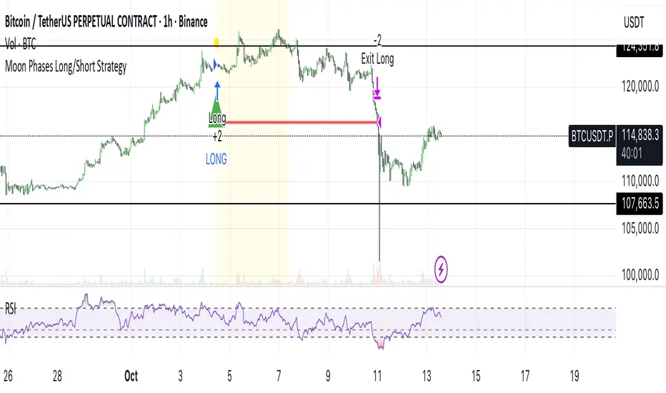
Moon Phases Long/Short StrategyThis is an experiment of Moon Phases, likely buy when full moon and sell when new moon with few changes, like it would buy a day ahead or sometimes sell a day post these events, with Stop loss and take profits, 50% profitable so sounds good to me
Long only good for bitcoin gold, both modes(L+S) better for stocks and alt coins
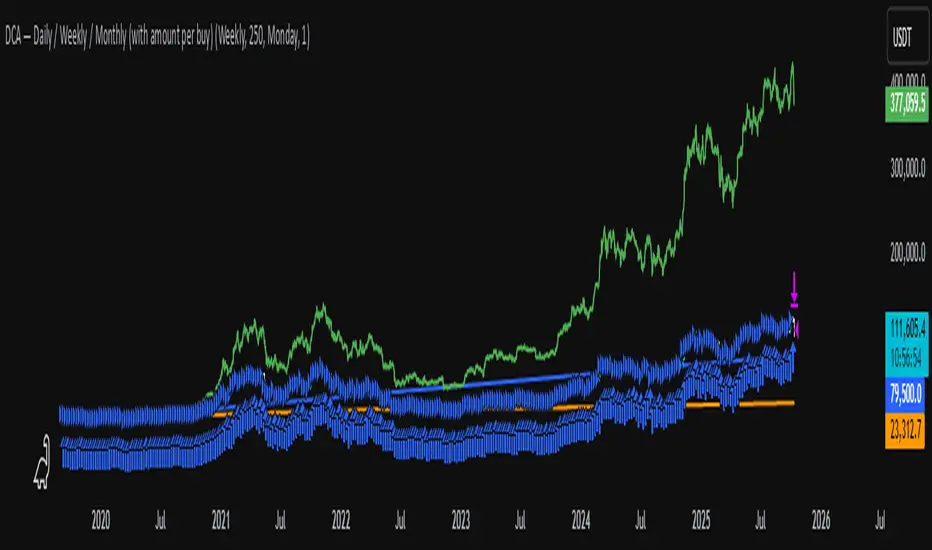
DCA Test Daily / Weekly / Monthly1.Input daily, weekly or monthly preferance of DCA
2.Select how much to DCA
3.Use the slider on the indicator down to select from where to DCA
Important: Don't use a higher timeframe chart than the desired DCA frequency, or all the DCA buys won't get executed.
Zero Lag + Momentum Bias StrategyZero Lag + Momentum Bias Strategy (MTF + Strong MBI + R:R + Partial TP + Alerts)

Strategy Builderuse external indicators on the chart as a source for a strategy. use 5 different triggers with drop down conditions. you can use any indicator that plots.
I will amend info when I get more time. improvement suggestions or indicator combinations would be appreciated.

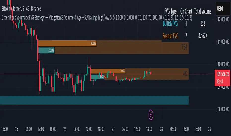
Order Block Volumatic FVG StrategyInspired by: Volumatic Fair Value Gaps —
License: CC BY-NC-SA 4.0 (Creative Commons Attribution–NonCommercial–ShareAlike).
This script is a non-commercial derivative work that credits the original author and keeps the same license.
What this strategy does
This turns BigBeluga’s visual FVG concept into an entry/exit strategy. It scans bullish and bearish FVG boxes, measures how deep price has mitigated into a box (as a percentage), and opens a long/short when your mitigation threshold and filters are satisfied. Risk is managed with a fixed Stop Loss % and a Trailing Stop that activates only after a user-defined profit trigger.
Additions vs. the original indicator
✅ Strategy entries based on % mitigation into FVGs (long/short).
✅ Lower-TF volume split using upticks/downticks; fallback if LTF data is missing (distributes prior bar volume by close’s position in its H–L range) to avoid NaN/0.
✅ Per-FVG total volume filter (min/max) so you can skip weak boxes.
✅ Age filter (min bars since the FVG was created) to avoid fresh/immature boxes.
✅ Bull% / Bear% share filter (the 46%/53% numbers you see inside each FVG).
✅ Optional candle confirmation and cooldown between trades.
✅ Risk management: fixed SL % + Trailing Stop with a profit trigger (doesn’t trail until your trigger is reached).
✅ Pine v6 safety: no unsupported args, no indexof/clamp/when, reverse-index deletes, guards against zero/NaN.
How a trade is decided (logic overview)
Detect FVGs (same rules as the original visual logic).
For each FVG currently intersected by the bar, compute:
Mitigation % (how deep price has entered the box).
Bull%/Bear% split (internal volume share).
Total volume (printed on the box) from LTF aggregation or fallback.
Age (bars) since the box was created.
Apply your filters:
Mitigation ≥ Long/Short threshold.
Volume between your min and max (if enabled).
Age ≥ min bars (if enabled).
Bull% / Bear% within your limits (if enabled).
(Optional) the current candle must be in trade direction (confirm).
If multiple FVGs qualify on the same bar, the strategy uses the most recent one.
Enter long/short (no pyramiding).
Exit with:
Fixed Stop Loss %, and
Trailing Stop that only starts after price reaches your profit trigger %.
Input settings (quick guide)
Mitigation source: close or high/low. Use high/low for intrabar touches; close is stricter.
Mitigation % thresholds: minimal mitigation for Long and Short.
TOTAL Volume filter: skip FVGs with too little/too much total volume (per box).
Bull/Bear share filter: require, e.g., Long only if Bull% ≥ 50; avoid Short when Bull% is high (Short Bull% max).
Age filter (bars): e.g., ≥ 20–30 bars to avoid fresh boxes.
Confirm candle: require candle direction to match the trade.
Cooldown (bars): minimum bars between entries.
Risk:
Stop Loss % (fixed from entry price).
Activate trailing at +% profit (the trigger).
Trailing distance % (the trailing gap once active).
Lower-TF aggregation:
Auto: TF/Divisor → picks 1/3/5m automatically.
Fixed: choose 1/3/5/15m explicitly.
If LTF can’t be fetched, fallback allocates prior bar’s volume by its close position in the bar’s H–L.
Suggested starting presets (you should optimize per market)
Mitigation: 60–80% for both Long/Short.
Bull/Bear share:
Long: Bull% ≥ 50–70, Bear% ≤ 100.
Short: Bull% ≤ 60 (avoid shorting into strong support), Bear% ≥ 0–70 as you prefer.
Age: ≥ 20–30 bars.
Volume: pick a min that filters noise for your symbol/timeframe.
Risk: SL 4–6%, trailing trigger 1–2%, distance 1–2% (crypto example).
Set slippage/fees in Strategy Properties.
Notes, limitations & best practices
Data differences: The LTF split uses request.security_lower_tf. If the exchange/data feed has sparse LTF data, the fallback kicks in (it’s deliberate to avoid NaNs but is a heuristic).
Real-time vs backtest: The current bar can update until close; results on historical bars use closed data. Use “Bar Replay” to understand intrabar effects.
No pyramiding: Only one position at a time. Modify pyramiding in the header if you need scaling.
Assets: For spot/crypto, TradingView “volume” is exchange volume; in some markets it may be tick volume—interpret filters accordingly.
Risk disclosure: Past performance ≠ future results. Use appropriate position sizing and risk controls; this is not financial advice.
Credits
Visual FVG concept and original implementation: BigBeluga.
This derivative strategy adds entry/exit logic, volume/age/share filters, robust LTF handling, and risk management while preserving the original spirit.
License remains CC BY-NC-SA 4.0 (non-commercial, attribution required, share-alike).
KD The ScalperWe have to take the trade when all three EMAs are pointing in the same direction (no criss-cross, no up/down, sideways). All 3 EMAs should be cleanly separated from each other with strong spacing between them; they are not tangled, sideways, or messy. This is our first filter before entering the trade. Are the EMAs stacked neatly, and is the price outside of the 25 EMA? If price pulls back and closes near or below the 25 or 50 EMA and breaks the 100 EMA, we don't trade. Use the 100 EMA as a safety net and refrain from trading if the price touches or falls below the 100 EMA.
1. Confirm the trend- All 3 EMAs must align, and they must spread
2. Watch price pull back to the 25th or the 50 EMA
3. Wait for the price to bounce - And re-approach the 25 EMA
Why is this powerful?
Removes 80% of the low-probability Trades
It keeps you out of choppy markets
Avoids Reversal Traps
Anchors us to momentum
We take the entry when the price moves up again and touches the 25 EMA from below, and then when it breaks above the 25 EMA, or even better, when a lovely green bullish candle forms. A bullish candle indicates good momentum. When a bullish candle closes in green, it means the momentum has increased significantly. This is when we enter a long trade, with the stop-loss just below the 50 EMA and the profit target being 1.5 times the stop-loss.
The same rule applies to the bearish trade.

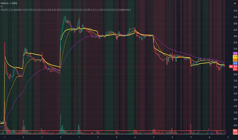
AVGO Advanced Day Trading Strategy📈 Overview
The AVGO Advanced Day Trading Strategy is a comprehensive, multi-timeframe trading system designed for active day traders seeking consistent performance with robust risk management. Originally optimized for AVGO (Broadcom), this strategy adapts well to other liquid stocks and can be customized for various trading styles.
🎯 Key Features
Multiple Entry Methods
EMA Crossover: Classic trend-following signals using fast (9) and medium (16) EMAs
MACD + RSI Confluence: Momentum-based entries combining MACD crossovers with RSI positioning
Price Momentum: Consecutive price action patterns with EMA and RSI confirmation
Hybrid System: Advanced multi-trigger approach combining all methodologies
Advanced Technical Arsenal
When enabled, the strategy analyzes 8+ additional indicators for confluence:
Volume Price Trend (VPT): Measures volume-weighted price momentum
On-Balance Volume (OBV): Tracks cumulative volume flow
Accumulation/Distribution Line: Identifies institutional money flow
Williams %R: Momentum oscillator for entry timing
Rate of Change Suite: Multi-timeframe momentum analysis (5, 14, 18 periods)
Commodity Channel Index (CCI): Cyclical turning points
Average Directional Index (ADX): Trend strength measurement
Parabolic SAR: Dynamic support/resistance levels
🛡️ Risk Management System
Position Sizing
Risk-based position sizing (default 1% per trade)
Maximum position limits (default 25% of equity)
Daily loss limits with automatic position closure
Multiple Profit Targets
Target 1: 1.5% gain (50% position exit)
Target 2: 2.5% gain (30% position exit)
Target 3: 3.6% gain (20% position exit)
Configurable exit percentages and target levels
Stop Loss Protection
ATR-based or percentage-based stop losses
Optional trailing stops
Dynamic stop adjustment based on market volatility
📊 Technical Specifications
Primary Indicators
EMAs: 9 (Fast), 16 (Medium), 50 (Long)
VWAP: Volume-weighted average price filter
RSI: 6-period momentum oscillator
MACD: 8/13/5 configuration for faster signals
Volume Confirmation
Volume filter requiring 1.6x average volume
19-period volume moving average baseline
Optional volume confirmation bypass
Market Structure Analysis
Bollinger Bands (20-period, 2.0 multiplier)
Squeeze detection for breakout opportunities
Fractal and pivot point analysis
⏰ Trading Hours & Filters
Time Management
Configurable trading hours (default: 9:30 AM - 3:30 PM EST)
Weekend and holiday filtering
Session-based trade management
Market Condition Filters
Trend alignment requirements
VWAP positioning filters
Volatility-based entry conditions
📱 Visual Features
Information Dashboard
Real-time display of:
Current entry method and signals
Bullish/bearish signal counts
RSI and MACD status
Trend direction and strength
Position status and P&L
Volume and time filter status
Chart Visualization
EMA plots with customizable colors
Entry signal markers
Target and stop level lines
Background color coding for trends
Optional Bollinger Bands and SAR display
🔔 Alert System
Entry Alerts
Customizable alerts for long and short entries
Method-specific alert messages
Signal confluence notifications
Advanced Alerts
Strong confluence threshold alerts
Custom alert messages with signal counts
Risk management alerts
⚙️ Customization Options
Strategy Parameters
Enable/disable long or short trades
Adjustable risk parameters
Multiple entry method selection
Advanced indicator on/off toggle
Visual Customization
Color schemes for all indicators
Dashboard position and size options
Show/hide various chart elements
Background color preferences
📋 Default Settings
Initial Capital: $100,000
Commission: 0.1%
Default Position Size: 10% of equity
Risk Per Trade: 1.0%
RSI Length: 6 periods
MACD: 8/13/5 configuration
Stop Loss: 1.1% or ATR-based
🎯 Best Use Cases
Day Trading: Designed for intraday opportunities
Swing Trading: Adaptable for longer-term positions
Momentum Trading: Excellent for trending markets
Risk-Conscious Trading: Built-in risk management protocols
⚠️ Important Notes
Paper Trading Recommended: Test thoroughly before live trading
Market Conditions: Performance varies with market volatility
Customization: Adjust parameters based on your risk tolerance
Educational Purpose: Use as a learning tool and customize for your needs
🏆 Performance Features
Detailed performance metrics
Trade-by-trade analysis capability
Customizable risk/reward ratios
Comprehensive backtesting support
This strategy is for educational purposes. Past performance does not guarantee future results. Always practice proper risk management and consider your financial situation before trading.
Ajay Nayak - EMA ATR Trailinge strategy RSI aur RSI ke SMA ke crossover par CALL aur PUT signal generate karti hai.
Saath me ATR based stoploss aur crossover target bhi diya gaya hai.
Algo trading ke liye useful hai.

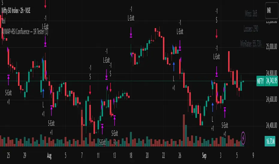
AVWAP+RSI Confluence — 1R TesterRSI + 1R ATR - Monthly P\&L (v4)
WHAT THIS STRATEGY DOES (OVERVIEW)
* Pine strategy (v4) that combines a simple momentum trigger with a symmetric 1R ATR risk model and an on-chart Monthly/Yearly P\&L table.
* Momentum filter: trades only when RSI crosses its own SMA in the direction of the trend (price vs Trend EMA).
* Risk engine: exits use fixed 1R ATR brackets captured at entry (no drifting targets/stops).
* Accounting: the table aggregates percentage returns by month and year using strategy equity.
ENTRY LOGIC (LONGS & OPTIONAL SHORTS)
Indicators used:
* RSI(rsiLen) and its SMA: SMA(RSI, rsiMaLen)
* Trend filter: EMA(emaTrendLen) on price
Longs:
1. RSI crosses above its RSI SMA
2. RSI > rsiBuyThr (filters weak momentum)
3. Close > EMA(emaTrendLen)
Shorts (optional via enableShort):
1. RSI crosses below its RSI SMA
2. RSI < rsiSellThr
3. Close < EMA(emaTrendLen)
EXIT LOGIC AND RISK MODEL (1R ATR)
* On entry, snapshot ATR(atrLen) into atrAtEntry and the average fill price into entryPx.
* Longs: stop = entryPx - ATR \* atrMult; target = entryPx + ATR \* atrMult
* Shorts: mirrored.
* Stops and targets are posted immediately and remain fixed for the life of the trade.
POSITION SIZING AND COSTS
* Default position size: 25% of equity per trade (adjustable in Properties/inputs).
* Commission percent and a small slippage are set in strategy() so backtests include friction by default.
MONTHLY / YEARLY P\&L TABLE (HOW IT WORKS)
* Uses strategy equity to compute bar returns: equity / equity\ - 1.
* Compounds bar returns into current month and current year; commits each finished period at month/year change (or last bar).
* Renders rows as years; columns Jan..Dec plus a Year total column.
* Cells colored by sign; precision and maximum rows are controlled by inputs.
* Values represent percentage returns, not currency P\&L.
VISUAL AIDS
* Two pivot trails (pivot high/low) are plotted for context only; they do not affect entries or exits.
CUSTOMIZATION TIPS
* Raise rsiBuyThr (long) or lower rsiSellThr (short) to filter weak momentum.
* Increase emaTrendLen to tighten trend alignment.
* Adjust atrLen and atrMult to fit your timeframe/instrument volatility.
* Leave enableShort = false if you prefer long-only behavior or shorting is constrained.
NON-REPAINTING AND BACKTEST NOTES
* Signals use bar-close crosses of built-in indicators (RSI, EMA, ATR); no future bars are referenced.
* calc\_on\_every\_tick = true for responsive visuals; Strategy Tester evaluates on bar close in history.
* Backtest stop/limit fills are simulated and may differ from live execution/liquidity.
DISCLAIMERS
* Educational use only. This is not financial advice. Markets involve risk. Past performance does not guarantee future results.
INPUTS (QUICK REFERENCE)
* rsiLen, rsiMaLen, rsiBuyThr, rsiSellThr
* emaTrendLen
* atrLen, atrMult, enableShort
* leftBars, rightBars, prec, showTable, maxYearsRows
SHORT TAGLINE
RSI momentum with 1R ATR brackets and a built-in Monthly/Yearly P\&L table.
TAGS
strategy, RSI, ATR, trend, risk-management, backtest, Pine-v4
Universal Webhook Connector Demo.This strategy demonstrates how to generate JSON alerts from TradingView for multiple trading platforms.
Users can select platform_name (MT5, TradeLocker, DxTrade, cTrader, etc).
Alerts are constructed in JSON format for webhook execution.

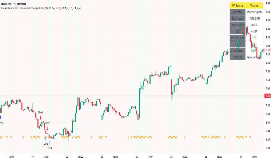
EMA inFusion Pro - Multiple SourcesEMA Fusion Pro: Dynamic Trend & Momentum Strategy with Three Exit Modes
EMA Fusion Pro is a highly customizable, multi-exit trend-following strategy designed for traders who value both precision and flexibility. By leveraging exponential moving averages (EMA), average directional index (ADX), and volume analysis, this strategy aims to capture trending market moves while offering three distinct exit modes for optimal risk management across varying market conditions.
Strategy Overview
This strategy systematically identifies potential entry points using a moving average crossover with highly configurable data sources (including price, volume, rate of change, or their Heikin Ashi versions) and filters signal quality with ADX trend strength and volume spikes. Each trade is managed with one of three advanced exit methodologies—reverse signal, ATR-based stop/take profit, or fixed percentage—giving you the control to adapt your risk profile to different market regimes.
Key Features
Customizable EMA Source: Calculate the core trend-filtering EMA from price (default), volume, rate of change, or their Heikin Ashi counterparts for unique market perspectives.
Trend Filter with ADX: Confirm entries only when the trend is strong, as measured by the user-adjustable ADX threshold.
Volume Spike Confirmation: Optional filter to only take trades with above-average volume activity, reducing false signals.
Three Exit Modes:
Reverse Signal: Exit trades when a new, opposite entry signal occurs.
ATR-Based Stop/Take Profit: Dynamic risk management using multiples of the average true range (ATR) for both take profit and stop loss.
Percent-Based Stop/Take Profit: Fixed-percentage risk management with user-defined thresholds.
Visual Annotations: Signal markers, EMA line color-coded by source, trend background coloring, and optional ATR/percent-based TP/SL levels.
Info Panel: Real-time display of all core indicators, current trading mode, exit parameters, and position status for quick oversight.
How It Works
Entry Logic: A crossover signal (above/below the EMA) triggers a new entry, but only if both ADX trend strength and (optionally) volume spike conditions are met.
Exit Logic: Three selectable modes allow you to exit trades on reverse signals, at a dynamic ATR-based profit or loss, or at a fixed percentage gain/loss.
Flexible Data Analysis: The EMA source can be chosen from six options—standard price, volume, rate of change, or their Heikin Ashi variants—allowing experimentation with different market dimensions.
Risk Management: All exits are precisely controlled, either by the next opposing signal, by volatility-adjusted levels, or by fixed risk/reward ratios.
Backtest & Optimization: The strategy is fully backtestable within TradingView’s Strategy Tester, with adjustable parameters for optimization.
Customization & Usage
Indicator Source: Select your preferred data type for EMA calculation, opening the door to creative strategy variations (e.g., volume momentum, pure price trend, rate of change divergence).
Filter Toggles: Enable/disable ADX and volume filters as desired—useful for different market environments.
Exit Mode Selection: Switch between reverse, ATR, or percent-based exits with a single parameter—ideal for adapting to ranging vs. trending markets.
Visual Clarity: The EMA line color reflects its underlying source, and the info panel summarizes all critical values for easy monitoring.
Who Should Use This Strategy?
Trend Followers seeking to ride strong moves with multiple exit options.
Experienced Traders who want to experiment with different data types (volume, momentum, Heikin Ashi) for trend analysis.
Algorithmic Traders looking for a robust, flexible base to build upon with their own ideas.
Getting Started
Apply the script to your chart and review default settings.
Customize parameters—EMA length, ADX threshold, volume settings, exit type—as desired.
Backtest on multiple instruments and timeframes to evaluate performance.
Optimize filters, exit rules, and risk parameters for your preferred trading style.
Monitor with the real-time info panel and trade alerts.
Disclaimer
This script is for educational and entertainment purposes only. It is not financial advice. Past performance is not indicative of future results. Always conduct thorough testing and consider your risk tolerance before trading real capital.
— Happy Trading —
Feel free to adapt, share, and contribute to this open-source strategy!
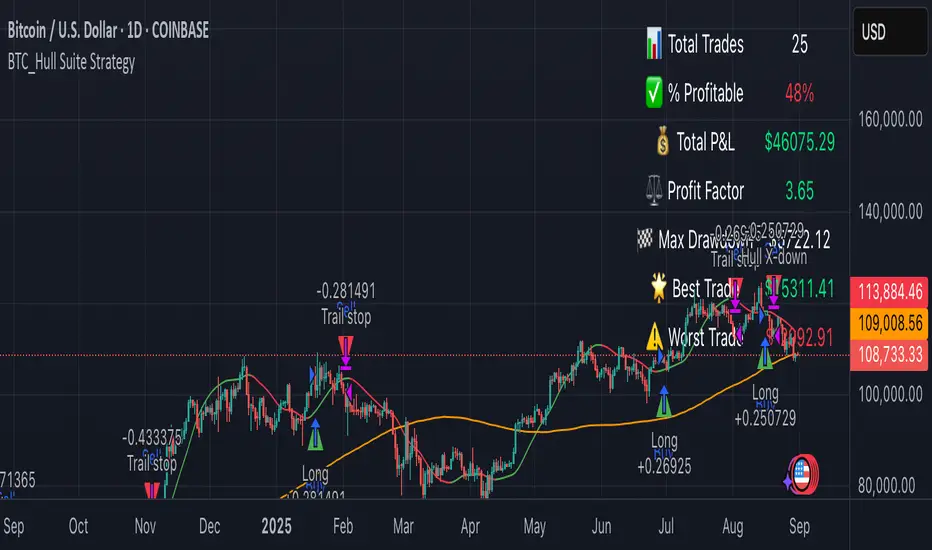
BTC_Hull Suite StrategyOverview
BTC_Hull Suite Strategy is a trend-following system designed to keep drawdowns modest while staying exposed during genuine uptrends. It uses the Hull Moving Average (HMA) for fast, low-lag trend turns, a long-term SMA filter to avoid chop, and a percentage trailing stop to protect gains.
🔧 What the strategy includes
- Hull Moving Average (HMA) with configurable length (default 55)
- SMA filter (default 130) to trade only with higher-timeframe bias
- Trailing stop in percent (default 5%) based on the running peak of close
- Execution model: signals are evaluated on the previous bar and entries are placed at the next bar’s open (TradingView default)
📈 How it works:
✅ Entry (Long):
Detects a bullish Hull turn by comparing the current HMA to its value 3 bars ago:
h > h3 and h <= h3 → HMA just turned up on the prior bar
The SMA filter must confirm: close > sma
If both are true (and within the date window), a long is opened next bar at the open
❌ Exit:
Hull turn down: h < h3 and h >= h3 , or
Trailing stop: price closes below peak * (1 – trailingPct)
Either condition closes the position at the current bar’s close
Notes:
pyramiding = 1 → allows one add-on (maximum two concurrent long positions)
Position sizing defaults to 20% of equity per entry (adjustable in Properties)
Who is this for?
This strategy is tailored for Bitcoin traders (spot or perpetuals) who want a rules-based, low-lag trend system with built-in drawdown protection.
It works best on Daily or 4H charts, but parameters can be adapted for other timeframes.
⚠️ Disclaimer
This strategy is provided for educational and research purposes only.
It is not financial advice. Markets are risky — always test on your own data, include realistic fees/slippage, and forward-test before using real capital.
Stoch TraderSimple example strategy that has greater than 60% win rate on 1m, 3m, and 5m views. Using something as simple as this with leverage can produce decent returns within 15-30min. It's also very easy to lose money doing this.
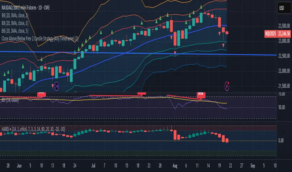
Close Above/Below Prev 2 Candle Strategy (Any Timeframe)Title: Close Above/Below Previous 2 Candle Strategy (Any Timeframe)
Description:
This strategy identifies potential breakout and trend continuation signals by analyzing the closing price relative to the highs and lows of the previous two candles. It works on any chart timeframe, making it versatile for intraday, swing, and daily trading.
How it works:
Long Entry (Bullish Signal): Triggered when the current candle closes above the highs of the previous two candles.
Short Entry (Bearish Signal): Triggered when the current candle closes below the lows of the previous two candles.
Visual Indicators:
Green triangles above the bar indicate bullish signals.
Red triangles below the bar indicate bearish signals.
Strategy Features:
Works on any timeframe, from 1-minute charts to daily/weekly charts.
Configurable risk/reward ratio for automatic stop-loss and take-profit levels.
Alerts trigger immediately when the condition is met, helping traders react to potential breakouts.
Provides clean visual signals for easy chart reading and decision-making.
Benefits:
Reduces noise by focusing on candle close confirmations.
Versatile and suitable for intraday, swing, and long-term trading.
Easy to combine with other indicators or strategies.
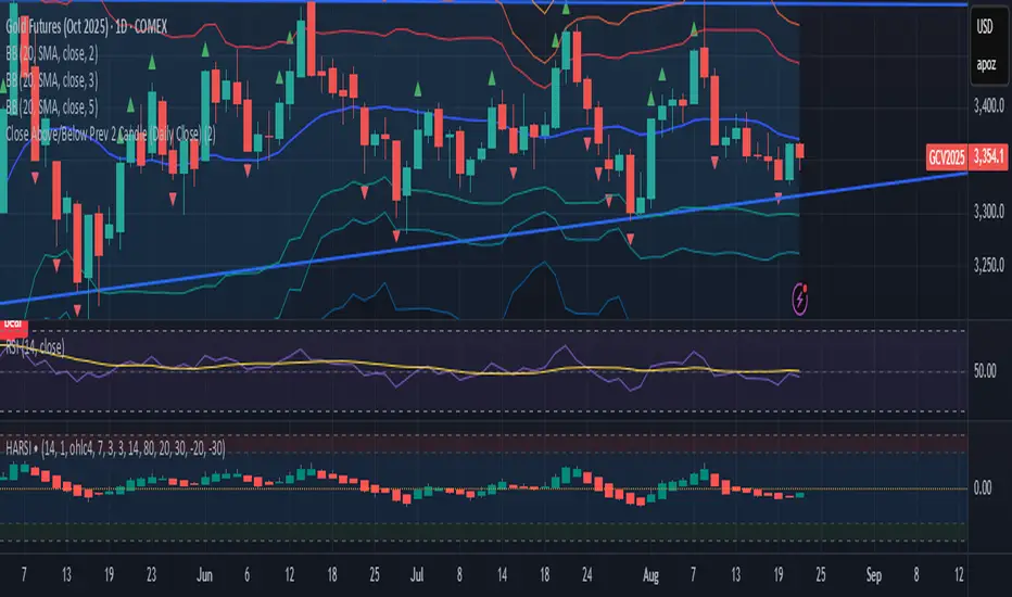
Close Above/Below Prev 2 Candle (Daily Close)This strategy identifies potential trend continuation or breakout signals by analyzing the daily candle closes relative to the previous two daily candles. It generates clear alerts and trade signals only after the daily candle has fully closed, reducing false intraday triggers.
How it works:
Long Entry (Bullish Signal): Triggered when the daily candle closes above the highs of the previous two daily candles.
Short Entry (Bearish Signal): Triggered when the daily candle closes below the lows of the previous two daily candles.
Visual Indicators: Green triangles indicate bullish signals, red triangles indicate bearish signals.
Strategy Features:
Optional long and short entries with configurable risk/reward ratio.
Automatic stop-loss and take-profit calculation based on candle structure.
Works on intraday charts using daily candle analysis.
Alerts:
Alerts trigger only after the daily candle closes above/below the previous two daily candles.
Helps traders receive precise notifications for potential breakout trades.
Benefits:
Reduces noise by using daily candle closes.
Easy to integrate with other swing or trend strategies.
Provides clear visual and alert signals for both bullish and bearish setups.
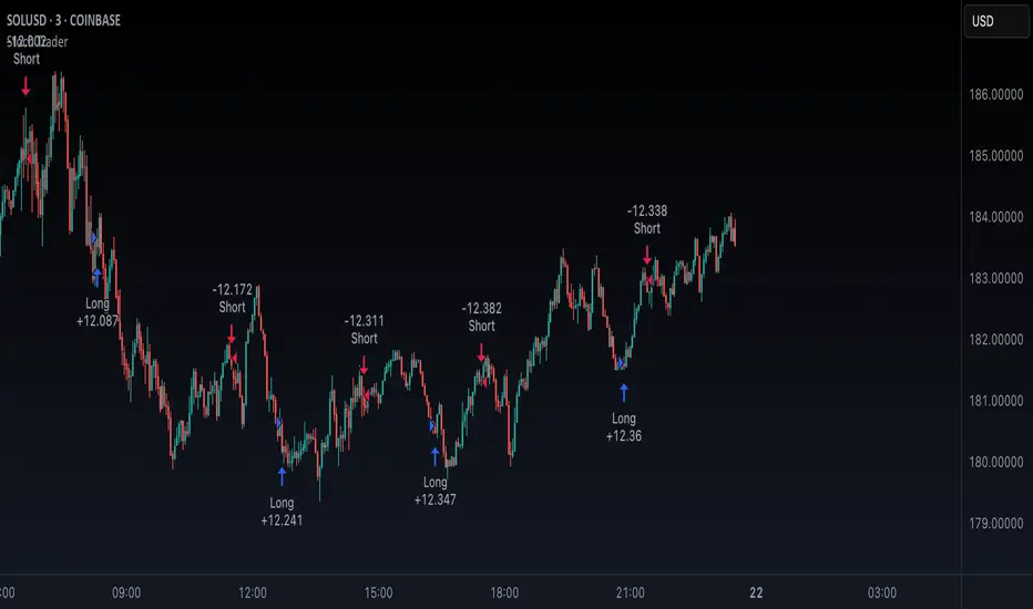
Scalping Line Strategy📌 Scalping Line Strategy – A Precision Crossover System
🔎 Overview
The Scalping Line Strategy is a short-term trading system built around the concept of momentum-driven crossovers between a smoothed moving average filter and a fast signal line. It is designed for scalpers and intraday traders who seek clear entry signals, minimal lag, and adaptive filtering to fit volatile market conditions.
At its core, the strategy uses a custom signal line ("Scalping Line"), which is derived from the difference between a double-smoothed moving average and a shorter-period signal line. Trade entries are triggered when this Scalping Line crosses above or below zero, providing a clean and rules-based framework for both long and short setups.
⚙️ Core Logic
Main Trend Filter – A double-smoothed moving average is calculated over a configurable period (default 100). This reduces noise and provides a more robust backbone for scalping signals.
Percent-Based Filter – To avoid false signals, a customizable percentage filter adjusts how closely the system “respects” price deviations from the moving average. This helps filter out insignificant fluctuations.
Signal Line – A shorter-period simple moving average (default 7) provides faster responsiveness to recent price action.
Scalping Line (SLI) – Calculated as the difference between the fast signal line and the smoothed moving average. When the SLI crosses zero, it signals a potential momentum shift.
SLI > 0 → Momentum bias is bullish.
SLI < 0 → Momentum bias is bearish.
🎯 Trade Direction & Flexibility
Trade Direction Control:
Choose between Long Only, Short Only, or Both to tailor the system to your trading style.
Signal Flip Option:
By default, long entries occur when the SLI crosses below zero, and shorts when it crosses above zero. This orientation can be flipped, allowing for alternative interpretations of the signals depending on how you want to capture momentum in your market.
🕒 Time Window Filtering
For intraday traders, a time filter can be enabled to restrict signals to specific trading sessions (e.g., 9 AM – 4 PM EST). This is particularly useful when trading assets such as equities or futures that have strong intraday volatility windows.
📈 Visuals & Clarity
Scalping Line Plot: Displayed as a dynamic oscillator around a zero baseline.
Histogram Fill: Green when above zero (bullish bias), red when below zero (bearish bias).
Signal Markers: Clear arrows mark long and short entries at crossover points.
Zero Line Reference: A flat gray line at zero assists in visually gauging momentum shifts.
🚀 Strategy Execution
Long Entry: Triggered when SLI crosses below zero (or above zero if flip is enabled) within allowed session hours.
Short Entry: Triggered when SLI crosses above zero (or below zero if flip is enabled) within allowed session hours.
Built-in Signal Cancels: Pending entries are canceled if conditions are no longer valid, ensuring no stale trades remain active.
✅ Best Use Cases
Markets: Works across equities, forex, crypto, and futures with sufficient intraday volatility.
Timeframes: Most effective on 1m to 15m charts for scalping setups, but adaptable to higher frames for swing trading.
Style: Traders who appreciate simple, rules-based momentum crossovers will find this system easy to follow and highly adaptable.
⚠️ Risk Management Note
This strategy is strictly an entry signal framework. Position sizing, stop-loss, and take-profit rules must be overlaid based on your risk management style. Always validate results with backtesting and forward testing before applying to live trading accounts.
📜 Final Thoughts
The Scalping Line Strategy offers a refined, easy-to-interpret approach to intraday trading. By combining smoothed moving averages, adaptive filtering, and flexible signal options, it helps traders identify short-term momentum shifts with clarity and confidence, making it a highly configurable tool for scalping-focused strategies.

Mutanabby_AI | Algo Pro Strategy# Mutanabby_AI | Algo Pro Strategy: Advanced Candlestick Pattern Trading System
## Strategy Overview
The Mutanabby_AI Algo Pro Strategy represents a systematic approach to automated trading based on advanced candlestick pattern recognition and multi-layered technical filtering. This strategy transforms traditional engulfing pattern analysis into a comprehensive trading system with sophisticated risk management and flexible position sizing capabilities.
The strategy operates on a long-only basis, entering positions when bullish engulfing patterns meet specific technical criteria and exiting when bearish engulfing patterns indicate potential trend reversals. The system incorporates multiple confirmation layers to enhance signal reliability while providing comprehensive customization options for different trading approaches and risk management preferences.
## Core Algorithm Architecture
The strategy foundation relies on bullish and bearish engulfing candlestick pattern recognition enhanced through technical analysis filtering mechanisms. Entry signals require simultaneous satisfaction of four distinct criteria: confirmed bullish engulfing pattern formation, candle stability analysis indicating decisive price action, RSI momentum confirmation below specified thresholds, and price decline verification over adjustable lookback periods.
The candle stability index measures the ratio between candlestick body size and total range including wicks, ensuring only well-formed patterns with clear directional conviction generate trading signals. This filtering mechanism eliminates indecisive market conditions where pattern reliability diminishes significantly.
RSI integration provides momentum confirmation by requiring oversold conditions before entry signal generation, ensuring alignment between pattern formation and underlying momentum characteristics. The RSI threshold remains fully adjustable to accommodate different market conditions and volatility environments.
Price decline verification examines whether current prices have decreased over a specified period, confirming that bullish engulfing patterns occur after meaningful downward movement rather than during sideways consolidation phases. This requirement enhances the probability of successful reversal pattern completion.
## Advanced Position Management System
The strategy incorporates dual position sizing methodologies to accommodate different account sizes and risk management approaches. Percentage-based position sizing calculates trade quantities as equity percentages, enabling consistent risk exposure across varying account balances and market conditions. This approach proves particularly valuable for systematic trading approaches and portfolio management applications.
Fixed quantity sizing provides precise control over trade sizes independent of account equity fluctuations, offering predictable position management for specific trading strategies or when implementing precise risk allocation models. The system enables seamless switching between sizing methods through simple configuration adjustments.
Position quantity calculations integrate seamlessly with TradingView's strategy testing framework, ensuring accurate backtesting results and realistic performance evaluation across different market conditions and time periods. The implementation maintains consistency between historical testing and live trading applications.
## Comprehensive Risk Management Framework
The strategy features dual stop loss methodologies addressing different risk management philosophies and market analysis approaches. Entry price-based stop losses calculate stop levels as fixed percentages below entry prices, providing predictable risk exposure and consistent risk-reward ratio maintenance across all trades.
The percentage-based stop loss system enables precise risk control by limiting maximum loss per trade to predetermined levels regardless of market volatility or entry timing. This approach proves essential for systematic trading strategies requiring consistent risk parameters and capital preservation during adverse market conditions.
Lowest low-based stop losses identify recent price support levels by analyzing minimum prices over adjustable lookback periods, placing stops below these technical levels with additional buffer percentages. This methodology aligns stop placement with market structure rather than arbitrary percentage calculations, potentially improving stop loss effectiveness during normal market fluctuations.
The lookback period adjustment enables optimization for different timeframes and market characteristics, with shorter periods providing tighter stops for active trading and longer periods offering broader stops suitable for position trading approaches. Buffer percentage additions ensure stops remain below obvious support levels where other market participants might place similar orders.
## Visual Customization and Interface Design
The strategy provides comprehensive visual customization through eight predefined color schemes designed for different chart backgrounds and personal preferences. Color scheme options include Classic bright green and red combinations, Ocean themes featuring blue and orange contrasts, Sunset combinations using gold and crimson, and Neon schemes providing high visibility through bright color selections.
Professional color schemes such as Forest, Royal, and Fire themes offer sophisticated alternatives suitable for business presentations and professional trading environments. The Custom color scheme enables precise color selection through individual color picker controls, maintaining maximum flexibility for specific visual requirements.
Label styling options accommodate different chart analysis preferences through text bubble, triangle, and arrow display formats. Size adjustments range from tiny through huge settings, ensuring appropriate visual scaling across different screen resolutions and chart configurations. Text color customization maintains readability across various chart themes and background selections.
## Signal Quality Enhancement Features
The strategy incorporates signal filtering mechanisms designed to eliminate repetitive signal generation during choppy market conditions. The disable repeating signals option prevents consecutive identical signals until opposing conditions occur, reducing overtrading during consolidation phases and improving overall signal quality.
Signal confirmation requirements ensure all technical criteria align before trade execution, reducing false signal occurrence while maintaining reasonable trading frequency for active strategies. The multi-layered approach balances signal quality against opportunity frequency through adjustable parameter optimization.
Entry and exit visualization provides clear trade identification through customizable labels positioned at relevant price levels. Stop loss visualization displays active risk levels through colored line plots, ensuring complete transparency regarding current risk management parameters during live trading operations.
## Implementation Guidelines and Optimization
The strategy performs effectively across multiple timeframes with optimal results typically occurring on intermediate timeframes ranging from fifteen minutes through four hours. Higher timeframes provide more reliable pattern formation and reduced false signal occurrence, while lower timeframes increase trading frequency at the expense of some signal reliability.
Parameter optimization should focus on RSI threshold adjustments based on market volatility characteristics and candlestick pattern timeframe analysis. Higher RSI thresholds generate fewer but potentially higher quality signals, while lower thresholds increase signal frequency with corresponding reliability considerations.
Stop loss method selection depends on trading style preferences and market analysis philosophy. Entry price-based stops suit systematic approaches requiring consistent risk parameters, while lowest low-based stops align with technical analysis methodologies emphasizing market structure recognition.
## Performance Considerations and Risk Disclosure
The strategy operates exclusively on long positions, making it unsuitable for bear market conditions or extended downtrend periods. Users should consider market environment analysis and broader trend assessment before implementing the strategy during adverse market conditions.
Candlestick pattern reliability varies significantly across different market conditions, with higher reliability typically occurring during trending markets compared to ranging or volatile conditions. Strategy performance may deteriorate during periods of reduced pattern effectiveness or increased market noise.
Risk management through stop loss implementation remains essential for capital preservation during adverse market movements. The strategy does not guarantee profitable outcomes and requires proper position sizing and risk management to prevent significant capital loss during unfavorable trading periods.
## Technical Specifications
The strategy utilizes standard TradingView Pine Script functions ensuring compatibility across all supported instruments and timeframes. Default configuration employs 14-period RSI calculations, adjustable candle stability thresholds, and customizable price decline verification periods optimized for general market conditions.
Initial capital settings default to $10,000 with percentage-based equity allocation, though users can adjust these parameters based on account size and risk tolerance requirements. The strategy maintains detailed trade logs and performance metrics through TradingView's integrated backtesting framework.
Alert integration enables real-time notification of entry and exit signals, stop loss executions, and other significant trading events. The comprehensive alert system supports automated trading applications and manual trade management approaches through detailed signal information provision.
## Conclusion
The Mutanabby_AI Algo Pro Strategy provides a systematic framework for candlestick pattern trading with comprehensive risk management and position sizing flexibility. The strategy's strength lies in its multi-layered confirmation approach and sophisticated customization options, enabling adaptation to various trading styles and market conditions.
Successful implementation requires understanding of candlestick pattern analysis principles and appropriate parameter optimization for specific market characteristics. The strategy serves traders seeking automated execution of proven technical analysis techniques while maintaining comprehensive control over risk management and position sizing methodologies.

MK Custome Adaptive SuperTrend Strategy [HalfSquatch]This strategy uses Lux Algos Adaptive supertrend. It has been modified here as a strategy.
This is used to test a trading bot.

Test Bot: Bearish Buy / Bullish SellFor testing the connection between TradingView and your brokerage. Use with a demo account if possible.

Day Trading Strategy (With Risk Management)This is a day trading strategy based on fast and slow EMA crossovers combined with RSI filtering to enhance trade accuracy. Designed for intraday use, it generates buy signals when the fast EMA crosses above the slow EMA and sell signals when it crosses below, but only if the RSI confirms momentum is favorable to avoid false entries in choppy markets.
The strategy includes built-in risk management with configurable stop-loss and take-profit levels set at 1% by default, helping to limit losses and secure profits quickly within the trading day. Clear buy and sell signals are plotted on the chart, and alerts notify traders in real time when trading opportunities arise.
Ideal for short-term traders, this system provides a disciplined, mechanical approach to capturing intraday trends with momentum confirmation and essential risk controls. It is fully customizable to fit different day trading instruments, timeframes, and risk appetites.

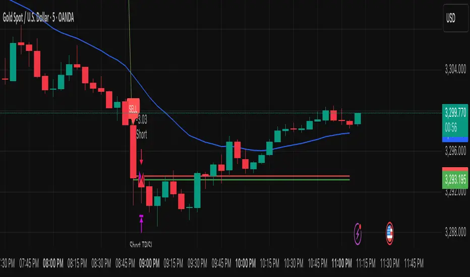
TPC Strategy XAUUSD - M5 with Fixed SL/TPThis script implements a trend-following strategy for XAUUSD on the 5-minute chart, using 200 EMA and 21 EMA to filter direction. Entries are triggered based on RSI, MACD crossovers, and price action alignment. It includes fixed Stop Loss (15 pips) and Take Profit (22.5 pips) with visual SL/TP lines, BUY/SELL labels, and alert conditions for automated notifications. Designed for intraday scalping and low-risk entries during trending conditions.
Combo 2/20 EMA & Bandpass Filter by TamarokDescription:
This strategy combines a 2/20 exponential moving average (EMA) crossover with a custom bandpass filter to generate buy and sell signals.
Use the Fast EMA and Slow EMA inputs to adjust trend sensitivity, and the Bandpass Filter Length, Delta, and Zones to fine-tune momentum turns.
Signals occur when both EMA and BPF agree in direction, with optional reversal and time filters.
How to use:
1. Add the script to your chart in TradingView.
2. Adjust the EMA and BP Filter parameters to match your asset’s volatility.
3. Enable ‘Reverse Signals’ to trade counter-trend, or use the time filter to limit sessions.
4. Set alerts on Long Alert and Short Alert for automated notifications.
Inspiration:
Based on HPotter’s original combo strategy (Stocks & Commodities Mar 2010).
Updated to Pine Script v6 with streamlined code and alerts.
WARNING:
For purpose educate only
