NQ Lunch High Low First Sweep StrategyThis script identifies the FIRST liquidity sweep of the Lunch session high or low
after the Lunch session has ended, based on ICT / Killzone concepts.
Logic summary:
• Tracks Lunch session High and Low (New York time)
• After Lunch session closes, monitors the market on 5-minute timeframe
• Triggers ONLY on the first sweep:
– Price wicks beyond Lunch High and closes back below → SHORT signal
– Price wicks beyond Lunch Low and closes back above → LONG signal
• Generates an alert at the exact bar where entry is expected
• Designed specifically for Nasdaq (NQ) futures
• One trade per day – no overtrading
Notes:
• Intended for 5-minute charts only
• Uses New York session timing
• This script does NOT manage exits (TP/SL) – entry logic only
• Best used as a confluence tool, not a standalone system
Educational & discretionary use only.
Educational

Supertrend + EMA + RSI Algo (Low Risk High Accuracy)This is a trend-following + momentum confirmation strategy designed to reduce false signals and control loss.
Supertrend (10,3) → Identifies overall market direction (Buy in uptrend, Sell in downtrend)
EMA 50 & EMA 200 → Confirms strong trend and avoids sideways market
Buy only when EMA 50 is above EMA 200
Sell only when EMA 50 is below EMA 200
RSI (14) → Confirms momentum
Buy when RSI > 55 (strong bullish momentum)
Sell when RSI < 45 (strong bearish momentum)
---
🔹 Entry Logic
BUY: Market is in uptrend + strong momentum
SELL: Market is in downtrend + strong bearish pressure
---
🔹 Risk Management (Most Important)
Stop Loss: Based on ATR (adapts to volatility)
Target: Fixed Risk-Reward ratio (example: 1 : 2.5)
This keeps loss small and profits larger
---
🔹 Best Use Case
Works best in trending markets
Ideal timeframes: 15m, 1h, 4h
Suitable for crypto futures & swing trading
Beginner-friendly if used with low leverage

225 SMA CrossoverWell-known strategy from Zahlengraf from the Mauerstrassenwetten subreddit for you to test yourself.
You can change the length of the SMA and whether to trade long, short or both directions.

Buy the dips StrategyThis strategy getting in long position only after the price drop- Buy the dips
The % of the drop is Determined by SMA for the first trade
The inputs of SMA and % of the drop can be adjust from the User
After that Strategy start taking safe trades if not take profit from the first trade
The safe trades are Determined by step down deviation % and by quantity
There is no Stop loss is not for one with small tolerance to getting under
if any question ask

Hybrid Trend-Following Inside Bar BreakoutHybrid Trend-Following Inside Bar Breakout Strategy
The Hybrid Trend-Following Inside Bar Breakout Strategy is a rule-based trading system designed to capture strong directional moves while controlling risk during uncertain market conditions. It combines trend-following, price action, and volatility-based risk management into a single robust framework.
Core Concept
The strategy trades inside bar breakouts only in the direction of the dominant market trend. Inside bars represent periods of consolidation, and when price breaks out of this consolidation in a trending market, it often leads to impulsive moves with favorable risk–reward characteristics.
Key Components
1. Trend Filter
Uses 50 EMA and 200 EMA to define the market trend.
Bullish bias: 50 EMA above 200 EMA
Bearish bias: 50 EMA below 200 EMA
This filter prevents counter-trend trades and improves trade quality.
2. Volatility Filter
Compares fast ATR (14) with slow ATR (50).
Trades are taken only when volatility is expanding or above a minimum threshold.
This avoids low-volatility, choppy market conditions.
3. Inside Bar Breakout
An inside bar forms when the current candle’s high is lower than the previous candle’s high and the low is higher than the previous candle’s low.
A trade is triggered only when price breaks above or below the inside bar range in the direction of the trend.
4. Candle Quality Filter
Requires a minimum body-to-range ratio, ensuring that the breakout candle has strong momentum and is not driven by weak wicks.
Risk Management & Trade Management
Stop Loss (SL)
Placed using ATR-based dynamic stops, adapting to current market volatility.
Prevents tight stops in volatile conditions and wide stops in calm markets.
Partial Profit Taking
50% of the position is exited at 1.5R, locking in profits early.
This reduces psychological pressure and improves equity stability.
Trailing Stop
After partial profit is taken, the remaining position is managed with an ATR-based trailing stop.
Allows the strategy to capture large trend moves while protecting gains.
Cooldown Mechanism
After a losing trade, the system enters a cooldown period and skips a fixed number of bars.
This helps avoid revenge trading and overtrading during unfavorable market phases.
Why This Strategy Works
Trades only high-probability breakouts in trending markets
Adapts automatically to changing volatility
Combines price action precision with systematic risk control
Designed for consistent performance over long historical periods

Buy-Dip / Sell-Pullback Buy the Dip / Sell the Pullback – Trend-Following Strategy (EOD → Next Day Execution)
Overview
This is a trend-following futures strategy designed to participate in pullbacks within established trends, not to predict reversals.
It works on End-of-Day (EOD) confirmation and executes trades on the next trading session, making it suitable for positional and swing traders.
The strategy combines momentum, trend direction, volatility, and price location to filter for high-quality setups while avoiding overtrading.
🔍 Core Philosophy
Trade only in the direction of the prevailing trend
Buy dips in uptrends
Sell pullbacks in downtrends
Avoid chasing price after extended gaps
Use volatility-adjusted risk management (ATR-based SL & targets)
📊 Indicators Used
RSI (20)
Measures underlying momentum strength
Stochastic Oscillator (55, 34, 21)
Confirms pullback exhaustion within a trend
Supertrend (10, 2)
Defines primary trend direction
Bollinger Bands (20, 2)
Provides structural trend bias
ATR (5)
Used for:
Entry gap filter
Stop-loss
Profit target
Supertrend buffer
✅ Long (Buy) Setup – Evaluated at EOD
A long setup is generated when all of the following conditions are satisfied at the close of the trading day:
RSI(20) is above the bullish threshold (default: 48)
Stochastic %K is above %D (confirming pullback momentum)
Supertrend direction is bullish
Price is near or above Supertrend, allowing a volatility-adjusted buffer (ATR-based)
Price is above the Bollinger Band middle line
This combination ensures:
The market is trending up
Momentum supports continuation
The pullback is controlled, not a breakdown
❌ Short (Sell) Setup – Evaluated at EOD
A short setup is generated when:
RSI(20) is below the bearish threshold (default: 52)
Stochastic %K is below %D
Supertrend direction is bearish
Price is near or below Supertrend, with an ATR buffer
Price is below the Bollinger Band middle line
This filters for pullbacks within sustained downtrends.
⏰ Trade Execution Logic (Next Day Rule)
Once a setup is confirmed at EOD, a trade is attempted on the next trading session
To avoid chasing gaps:
Long trades are allowed only if price does not move more than a defined multiple of the previous day’s True Range
Short trades follow the same logic in reverse
This is implemented via limit orders, ensuring realistic backtesting and execution behavior
🛑 Risk Management
All exits are volatility-adjusted using ATR:
Stop-Loss:
1.1 × ATR(5) from entry price
Target:
2.2 × ATR(5) from entry price
This results in a risk–reward ratio of approximately 1:2
ATR is frozen at entry to avoid forward-looking bias.
🧠 Why This Strategy Works
Avoids low-quality trades during consolidation
Participates only when trend + momentum align
Prevents emotional gap-chasing
Adapts automatically to changing volatility
Suitable for index futures and liquid stocks
📌 Recommended Usage
Timeframe: Daily
Instruments:
Index Futures (e.g. NIFTY, BANKNIFTY)
Highly liquid stocks
Market Type: Trending markets
Not ideal for: Sideways or low-volatility environments
⚙️ Customization Tips
You can control trade frequency and aggressiveness by adjusting:
RSI thresholds
Supertrend buffer (ATR multiple)
Gap filter multiplier
Stochastic edge parameter
Looser settings → more trades
Stricter settings → higher selectivity
⚠️ Disclaimer
This strategy is for educational and research purposes only.
Backtest results do not guarantee future performance.
Always validate with paper trading before deploying real capital.

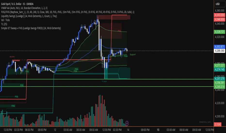
Simple ICT Sweep + FVG (LuxAlgo Swings FIXED)something i created if anyone can improve it or change for better visual
Slope Failure (Momentum Stall) STRATEGY//======================================================================================
// SLOPE FAILURE (MOMENTUM STALL) STRATEGY
//--------------------------------------------------------------------------------------
// WHAT THIS STRATEGY DOES
// -----------------------
// This strategy trades **momentum failure**, not trend direction.
//
// Instead of predicting where price will go, it detects when **momentum can no longer
// continue in its current direction** and briefly fades that failure.
//
// Core idea:
// - Momentum expands → slope grows
// - Momentum stalls → slope collapses or flips
// - That stall represents **state transition**, not noise
//
// The system exploits these transitions repeatedly at short horizons.
//
//--------------------------------------------------------------------------------------
// HOW MOMENTUM IS MEASURED
// ------------------------
// 1. Source price (optionally smoothed)
// 2. First derivative (slope = price - price )
// 3. Optional smoothing of the slope itself
//
// The slope represents **instantaneous directional force**, not trend bias.
//
//--------------------------------------------------------------------------------------
// ENTRY LOGIC (SLOPE FAILURE)
// ---------------------------
// • Bull Slope Failure (SHORT):
// - Prior slope was sufficiently positive
// - Current slope collapses to zero or below
// → Upward momentum failed → enter SHORT
//
// • Bear Slope Failure (LONG):
// - Prior slope was sufficiently negative
// - Current slope rises to zero or above
// → Downward momentum failed → enter LONG
//
// Optional:
// - Minimum slope band can be enforced to avoid weak/noisy failures
//
//--------------------------------------------------------------------------------------
// EXIT LOGIC
// ----------
// Primary exits are **force-based**, not price-based:
//
// • Longest Slope Local Turn (optional):
// - Detects when the strongest slope in a recent window has occurred
// - Exits when momentum starts decaying from that extreme
//
// • Percent Stop Loss (optional):
// - Fixed % protection relative to entry price
//
// The strategy does NOT rely on profit targets.
// Winners are exited when **momentum decays**, not when price "looks good".
//
//--------------------------------------------------------------------------------------
// POSITION SIZING
// ---------------
// This strategy supports **percent-of-equity sizing**, computed dynamically:
//
// position size = (account equity × % allocation) / price
//
// This allows:
// - P&L to scale smoothly
// - Drawdowns to remain proportional
// - The same logic to work across symbols and account sizes
//
//--------------------------------------------------------------------------------------
// STRATEGY CHARACTERISTICS
// ------------------------
// • High trade count
// • Win rate near ~45–50%
// • Small, fast losers
// • Slightly larger winners
// • Very low drawdown
//
// This profile is intentionally designed for **scalability**, not prediction.
//
//--------------------------------------------------------------------------------------
// IMPORTANT NOTES
// ---------------
// • This is NOT a trend-following strategy
// • This is NOT a mean-reversion guess
// • This is a momentum **state-transition detector**
//
// The edge comes from structure + exits + sizing — not indicators.
//
//======================================================================================

Mutanabby_AI | ONEUSDT_MR1
ONEUSDT Mean-Reversion Strategy | 74.68% Win Rate | 417% Net Profit
This is a long-only mean-reversion strategy designed specifically for ONEUSDT on the 1-hour timeframe. The core logic identifies oversold conditions following sharp declines and enters positions when selling pressure exhausts, capturing the subsequent recovery bounce.
Backtested Period: June 2019 – December 2025 (~6 years)
Performance Summary
| Metric | Value |
|--------|-------|
| Net Profit | +417.68% |
| Win Rate | 74.68% |
| Profit Factor | 4.019 |
| Total Trades | 237 |
| Sharpe Ratio | 0.364 |
| Sortino Ratio | 1.917 |
| Max Drawdown | 51.08% |
| Avg Win | +3.14% |
| Avg Loss | -2.30% |
| Buy & Hold Return | -80.44% |
Strategy Logic :
Entry Conditions (Long Only):
The strategy seeks confluence of three conditions that identify exhausted selling:
1. Prior Move Filter:*The price change from 5 bars ago to 3 bars ago must be ≥ -7% (ensures we're not entering during freefall)
2. Current Move Filter: The price change over the last 2 bars must be ≤ 0% (confirms momentum is stalling or reversing)
3. Three-Bar Decline: The price change from 5 bars ago to 3 bars ago must be ≤ -5% (confirms a significant recent drop occurred)
When all three conditions align, the strategy identifies a potential reversal point where sellers are exhausted.
Exit Conditions:
- Primary Exit: Close above the previous bar's high while the open of the previous bar is at or below the close from 9 bars ago (profit-taking on strength)
- Trailing Stop: 11x ATR trailing stop that locks in profits as price rises
Risk Management
- Position Sizing:Fixed position based on account equity divided by entry price
- Trailing Stop:11× ATR (14-period) provides wide enough room for crypto volatility while protecting gains
- Pyramiding:Up to 4 orders allowed (can scale into winning positions)
- **Commission:** 0.1% per trade (realistic exchange fees included)
Important Disclaimers
⚠️ This is NOT financial advice.
- Past performance does not guarantee future results
- Backtest results may contain look-ahead bias or curve-fitting
- Real trading involves slippage, liquidity issues, and execution delays
- This strategy is optimized for ONEUSDT specifically — results may differ on other pairs
- Always test before risking real capital
Recommended Usage
- Timeframe:*1H (as designed)
- Pair: ONEUSDT (Binance)
- Account Size: Ensure sufficient capital to survive max drawdown
Source Code
Feedback Welcome
I'm sharing this strategy freely for educational purposes. Please:
- Drop a comment with your backtesting results any you analysis
- Share any modifications that improve performance
- Let me know if you spot any issues in the logic
Happy trading
As a quant trader, do you think this strategy will survive in live trading?
Yes or No? And why?
I want to hear from you guys


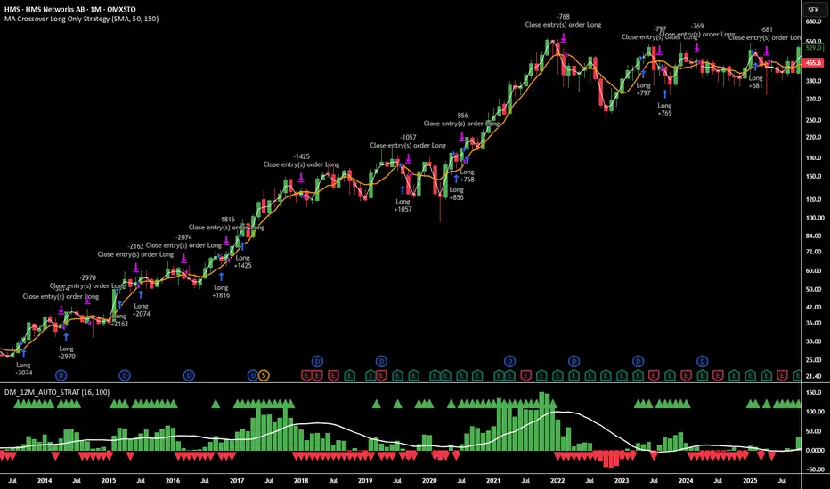
12M Return Strategy This strategy is based on the original Dual Momentum concept presented by Gary Antonacci in his book “Dual Momentum Investing.”
It implements the absolute momentum portion of the framework using a 12-month rate of change, combined with a moving-average filter for trend confirmation.
The script automatically adapts the lookback period depending on chart timeframe, ensuring the return calculation always represents approximately one year, whether you are on daily, weekly, or monthly charts.
How the Strategy Works
1. 12-Month Return Calculation
The core signal is the 12-month price return, computed as:
(Current Price ÷ Price from ~1 year ago) − 1
This return:
Plots as a histogram
Turns green when positive
Turns red when negative
The lookback adjusts automatically:
1D chart → 252 bars
1W chart → 52 bars
1M chart → 12 bars
Other timeframes → estimated to approximate 1 calendar year
2. Trend Filter (Moving Average of Return)
To smooth volatility and avoid noise, the strategy applies a moving average to the 12M return:
Default length: 12 periods
Plotted as a white line on the indicator panel
This becomes the benchmark used for crossovers.
3. Trade Signals (Long / Short / Cash)
Trades are generated using a simple crossover mechanism:
Bullish Signal (Go Long)
When:
12M Return crosses ABOVE its MA
Action:
Close short (if any)
Enter long
Bearish Signal (Go Short or Go Flat)
When:
12M Return crosses BELOW its MA
Action:
If shorting is enabled → Enter short
If shorting is disabled → Exit position and go to cash
Shorting can be enabled or disabled with a single input switch.
4. Position Sizing
The strategy uses:
Percent of Equity position sizing
You can specify the percentage of your portfolio to allocate (default 100%).
No leverage is required, but the strategy supports it if your account settings allow.
5. Visual Signals
To improve clarity, the strategy marks signals directly on the indicator panel:
Green Up Arrows: return > MA
Red Down Arrows: return < MA
A status label shows the current mode:
LONG
SHORT
CASH
6. Backtest-Ready
This script is built as a full TradingView strategy, not just an indicator.
This means you can:
Run complete backtests
View performance metrics
Compare long-only vs long/short behavior
Adjust inputs to tune the system
It provides a clean, rule-driven interpretation of the classic absolute momentum approach.
Inspired By: Gary Antonacci – Dual Momentum Investing
This script reflects the absolute momentum side of Antonacci’s original research:
Uses 12-month momentum (the most statistically validated lookback)
Applies a trend-following overlay to control downside risk
Recreates the classic signal structure used in academic studies
It is a simplified, transparent version intended for practical use and educational clarity.
Disclaimer
This script is for educational and research purposes only.
Historical performance does not guarantee future results.
Always use proper risk management.
Robrechtian Long-Medium Breakout Trend SystemRobrechtian Long–Medium-Term Breakout Trend System
A professional, rule-based trend-following strategy designed to capture large, sustained price movements using pure price action and breakouts.
This system follows long-established trend-following philosophy: no prediction, no volatility targeting, and no profit targets. Only disciplined entries, position additions, and exits driven entirely by trend structure.
Core Principles
Breakout-driven entries: Initial positions are taken only when price breaks above/below the 80-day Donchian channel, confirming a long–medium-term trend shift.
Short-term confirmation: Breakouts must also exceed the 20-day channel, reducing false positives.
Trend-direction filter: A 50-day moving average slope filter ensures alignment with the broader trend.
Explosive bar filter: Entries avoid excessively large, single-candle expansions (>2.5× ATR(20)) to prevent chasing exhaustion spikes.
Pyramiding into strength: Additional units are added only when price makes fresh 20-day breakouts in the direction of the trend. No scaling out. No adding on dips.
Exit only on trend violation: Positions are closed exclusively when price breaks the opposite 80-day channel. This preserves unlimited upside while enforcing disciplined exits.
Pure trend philosophy: No volatility targeting, no smoothing, no discretionary overrides, no optimization for short-term performance.
Intended Use
This system is designed primarily for diversified futures portfolios, where diversification across dozens of globally liquid markets creates robustness and stability. However, it may also be used on individual assets for educational and analytical purposes.
The system embraces the core trend-following logic:
Small losses, big winners, and unlimited upside when trends persist.
⚠️ WARNINGS / DISCLAIMERS
⚠️ Warning 1 — This strategy is not optimized for single stocks
The Robrechtian Trend System is designed for multi-asset futures portfolios, not single equities.
Performance on individual tickers may vary greatly due to lack of diversification.
⚠️ Warning 2 — Trend following includes substantial drawdowns
Deep drawdowns are a normal and expected feature of all long-term trend-following systems.
The strategy does not attempt to smooth returns or manage volatility.
If you seek steady, low-volatility equity curves, this system is not suitable.
⚠️ Warning 3 — No volatility targeting or risk smoothing
This system intentionally avoids volatility-based position sizing.
Trades may experience larger fluctuations than systems using risk parity or vol targeting.
⚠️ Warning 4 — Not financial advice
This script is for educational and research purposes only.
Past performance does not guarantee future results.
Use at your own risk.
⚠️ Warning 5 — TradingView backtests have known limitations
TradingView does not simulate:
futures contract roll logic
slippage
real bid/ask spreads
liquidity conditions
limit-up/limit-down behavior
Results may vary from live market execution.

NIFTY 5m/15m Smart Money CE/PE – High WinRatenice strategy for intraday NIFTY option trading. It works best on 5 minute time frame on NIFTY Index Chart

SSL ST Strategy – Accuracy Enhanced v2.0 (Parser Safe)This strategy is built to identify high-probability trend breakouts using a combination of SSL Channel, Baseline, Hull / EMA signals, and Candle-based confirmations.
The goal is to filter noise, avoid false breakouts, and enter only when the trend is truly shifting.
This strategy identifies high-probability trend breakouts using SSL Channel, Baseline, Hull/EMA, and candle
confirmations.
1. SSL shows trend shift when price breaks high/low levels.
2. Baseline filters direction (price above = buy bias, below = sell bias).
3. Hull/EMA gives early momentum confirmation.
4. Candle breakout ensures real momentum (breaks previous high/low).
5. Optional filters: ATR, reversal logic, continuation entries.
6. Exits occur on SSL flip, baseline cross, or weakness
Disclaimer
This strategy is provided strictly for educational and informational purposes only. It does not guarantee any profit, nor does it protect against losses of any kind. Financial markets are inherently unpredictable, and any market movement can only be assumed or estimated with a probability that is never guaranteed and can often be no better than a 50/50 chance.
By using this strategy, you acknowledge that all trading decisions are made solely at your own risk. I am not liable for any profits, losses, or financial consequences incurred by anyone using or relying on this strategy. Always perform your own research, manage your risk responsibly, and consult with a qualified financial advisor before trading.

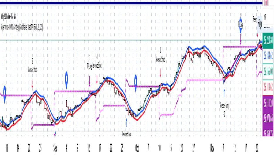
Supertrend + DEMA Strategy ( customised & Switchable, Fixed TP)Supertrend line – a moving line that follows the price and shows whether the market is trending up or down.
If the price goes above this line, it usually means the market is going up.
If the price goes below, it usually means the market is going down.
DEMA (Double Exponential Moving Average) – another line that smooths out price movements to spot trends more clearly.
It calculates an average of prices but reacts faster than a normal moving average.
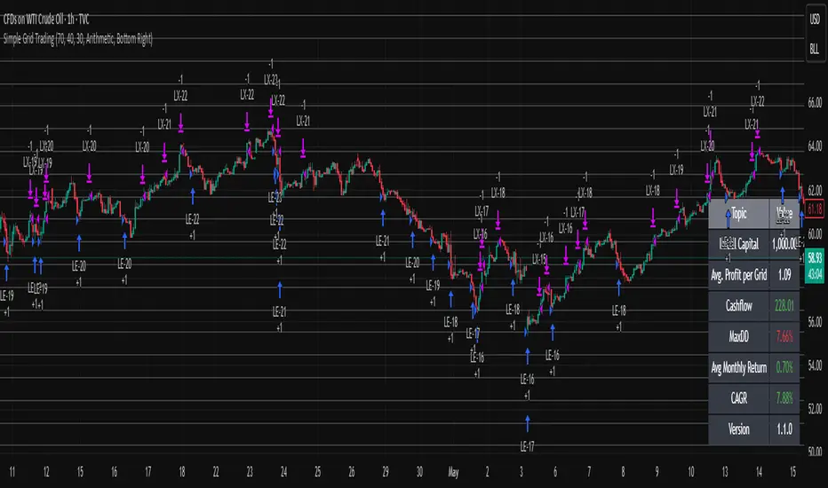
Simple Grid Trading v1.0 [PUCHON]Simple Grid Trading v1.0
Overview
This is a Long-Only Grid Trading Strategy developed in Pine Script v6 for TradingView. It is designed to profit from market volatility by placing a series of Buy Limit orders at predefined price levels. As the price drops, the strategy accumulates positions. As the price rises, it sells these positions at a profit.
Features
Grid Types : Supports both Arithmetic (equal price spacing) and Geometric (equal percentage spacing) grids.
Flexible Order Management : Uses strategy.order for precise control and prevents duplicate orders at the same level.
Performance Dashboard : A real-time table displaying key metrics like Capital, Cashflow, and Drawdown.
Advanced Metrics : Includes Max Drawdown (MaxDD) , Avg Monthly Return , and CAGR calculations.
Customizable : Fully adjustable price range, grid lines, and lot size.
Dashboard Metrics
The dashboard (default: Bottom Right) provides a quick snapshot of the strategy's performance:
Initial Capital : The starting capital defined in the strategy settings.
Lot Size : The fixed quantity of assets purchased per grid level.
Avg. Profit per Grid : The average realized profit for each closed trade.
Cashflow : The total realized net profit (closed trades only).
MaxDD : Maximum Drawdown . The largest percentage drop in equity (realized + unrealized) from a peak.
Avg Monthly Return : The average percentage return generated per month.
CAGR : Compound Annual Growth Rate . The mean annual growth rate of the investment over the specified time period.
Strategy Settings (Inputs)
Grid Settings
Upper Price : The highest price level for the grid.
Lower Price : The lowest price level for the grid.
Number of Grid Lines : The total number of levels (lines) in the grid.
Grid Type :
Arithmetic: Distance between lines is fixed in price terms (e.g., $10, $20, $30).
Geometric: Distance between lines is fixed in percentage terms (e.g., 1%, 2%, 3%).
Lot Size : The fixed amount of the asset to buy at each level.
Dashboard Settings
Show Dashboard : Toggle to hide/show the performance table.
Position : Choose where the dashboard appears on the chart (e.g., Bottom Right, Top Left).
How It Works
Initialization : On the first bar, the script calculates the price levels based on your Upper/Lower price and Grid Type.
Entry Logic :
The strategy places Buy Limit orders at every grid level below the current price.
It checks if a position already exists at a specific level to avoid "stacking" multiple orders on the same line.
Exit Logic :
For every Buy order, a corresponding Sell Limit (Take Profit) order is placed at the next higher grid level.
MaxDD Calculation :
The script continuously tracks the highest equity peak.
It calculates the drawdown on every bar (including intra-bar movements) to ensure accuracy.
Displayed as a percentage (e.g., 5.25%).
Disclaimer
This script is for educational and backtesting purposes only. Grid trading involves significant risk, especially in strong trending markets where the price may move outside your grid range. Always use proper risk management.
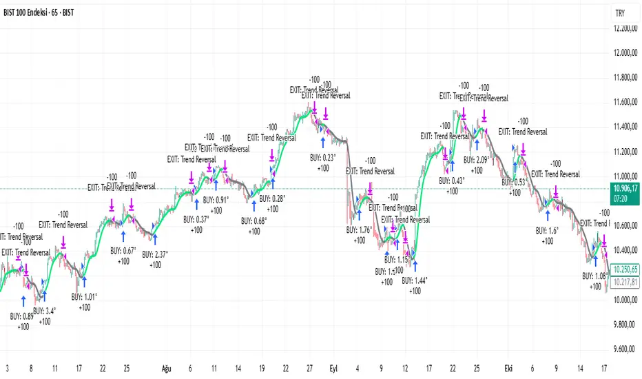
Recursive WMA Angle StrategyDescription: This strategy utilizes a recursive Weighted Moving Average (WMA) calculation to determine the trend direction and strength based on the slope (angle) of the curve. By calculating the angle of the smoothed moving average in degrees, the script filters out noise and aims to enter trades only during strong momentum phases.
How it Works:
Recursive WMA: The script calculates a series of nested WMAs (M1 to M5), creating a very smooth yet responsive curve.
Angle Calculation: It measures the rate of change of this curve over a user-defined lookback period and converts it into an angle (in degrees).
Entry Condition (Long): A long position is opened when the calculated angle exceeds the Min Angle for BUY threshold (default: 0.2), indicating a strong upward trend.
Exit Condition: The position is closed when the angle drops below the Min Angle for SELL threshold (default: -0.2), indicating a sharp trend reversal.
Settings:
MA Settings: Adjust the base lengths for the recursive calculation.
Angle Settings: Fine-tune the sensitivity by changing the Buy/Sell angle thresholds.
Date Filter: Restrict the backtest to a specific date range.
Note: This strategy is designed for Long-Only setups.
12M SMA Timing (HTF-safe, 100% equity)Buy when S&P500 closes above 12M moving average. Sell when it closes below it. Monthly only.

WIN1! • Crossing EMAs• (By Mesquita, v7)Moving average crossover strategy for intraday movements, especially in the continuous index (WIN1!) on the Brazilian stock exchange B³. The strategy is customizable for time windows, has a filter for trades only above the long-term average, whether only long, only short, or both, with or without stop loss.

KZ One — Scalping Training StrategyKZ One is a scalping strategy developed for M1 and M5 timeframes. It is designed to help traders study and practice short-term market behavior by using structured zones to highlight potential entry and exit areas. The strategy allows customization of Risk (USD) and Take Profit (R multiple) parameters for flexible trade management. Additional tools include ATR-based filters to skip low-volatility conditions and a Pre-Alert Lead (bars) option that notifies users ahead of possible setups. KZ One is intended for educational and analytical purposes, promoting disciplined and consistent trading practice.

💸 DCA Accumulation Strategy (USD‑Based Scaling)Buy when blue arrow appears, if the next arrow is lower than the last increase your position. This will pull your average cost down slowly over time.

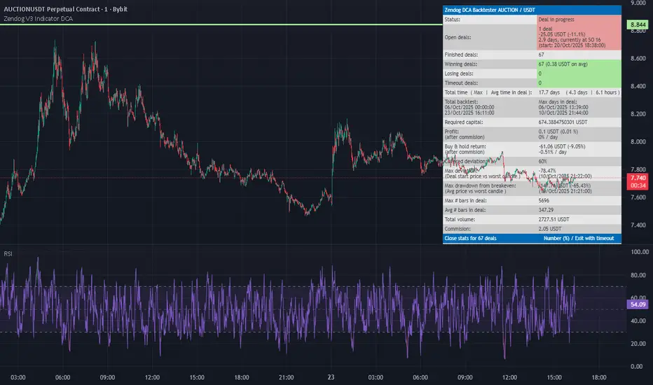
Zendog V3 Indicator DCAThis strategy is same as Zendog v3 but edited to be backtest compatible for SO additions through indicator
for Longs
Safety order type = External indicator
External indicator = RSI 30/70 : Long Trigger
Safety Order Value = 1
for Shorts
Safety order type = External indicator
External indicator = RSI 30/70 : Short Trigger
Safety Order Value = 2
Enhanced OB Retest Strategy v7.0The OB Retest Strategy is a full Order Block retest trading system that detects, plots, and trades OB zones across multiple timeframes. It uses structure breaks, retrace depth, and ATR filters to identify strong reversal or continuation setups.
⸻
⚙️ Core Features
• Multi-timeframe OB detection using break-of-structure (BOS) logic
• Automatic zone creation for bullish and bearish order blocks
• Smart merging of overlapping OB zones
• Dynamic flip-zone logic that turns invalidated OBs into new zones
• Wick zone detection for high-precision entries
• ATR-based trailing stop and optional breakeven
• Adjustable retrace depth, breakout %, and ATR filters
• Built-in performance table showing PnL, win rate, and total trades
• Fully backtestable with date range and commission control
⸻
🧠 Logic Summary
1. Detects a BOS on the higher timeframe.
2. Identifies the last opposing candle as the valid OB.
3. Validates the OB based on ATR size and breakout strength.
4. Waits for price to retest the zone to a set depth.
5. Executes trades and manages exits using trailing stop or breakeven.
6. Flips invalidated zones automatically.
⸻
💡 Usage Tips
• Best used on 1H to 4H charts for swing setups.
• Tune ATR and breakout thresholds for your market’s volatility.
• Combine with higher-timeframe bias or liquidity levels for better accuracy.
⸻
⚠️ Notes
• For educational and testing purposes only.
• Backtested results do not predict future performance.
• Always test before live use.
