Time-Price Velocity [QuantAlgo]🟢 Overview
The Time-Price Velocity indicator uses advanced velocity-based analysis to measure the rate of price change normalized against typical market movement, creating a dynamic momentum oscillator that identifies market acceleration patterns and momentum shifts. Unlike traditional momentum indicators that focus solely on price change magnitude, this indicator incorporates time-weighted displacement calculations and ATR normalization to create a sophisticated velocity measurement system that adapts to varying market volatility conditions.
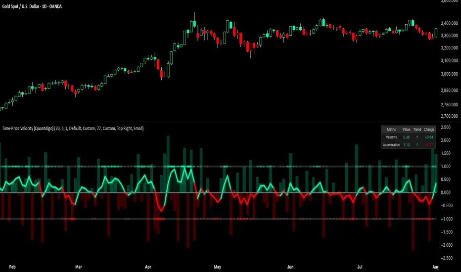
This indicator displays a velocity signal line that oscillates around zero, with positive values indicating upward price velocity and negative values indicating downward price velocity. The signal incorporates acceleration background columns and statistical normalization to help traders identify momentum shifts and potential reversal or continuation opportunities across different timeframes and asset classes.
🟢 How It Works
The indicator's key insight lies in its time-price velocity calculation system, where velocity is measured using the fundamental physics formula:
velocity = priceChange / timeWeight
The system normalizes this raw velocity against typical price movement using Average True Range (ATR) to create market-adjusted readings:
normalizedVelocity = typicalMove > 0 ? velocity / typicalMove : 0
where "typicalMove = ta.atr(lookback)" provides the baseline for normal price movement over the specified lookback period.
The Time-Price Velocity indicator calculation combines multiple sophisticated components. First, it calculates acceleration as the change in velocity over time:
acceleration = normalizedVelocity - normalizedVelocity
Then, the signal generation applies EMA smoothing to reduce noise while preserving responsiveness:
signal = ta.ema(normalizedVelocity, smooth)
This creates a velocity-based momentum indicator that combines price displacement analysis with statistical normalization, providing traders with both directional signals and acceleration insights for enhanced market timing.
🟢 How to Use
1. Signal Interpretation and Threshold Zones
Positive Values (Above Zero): Time-price velocity indicating bullish momentum with upward price displacement relative to normalized baseline
Negative Values (Below Zero): Time-price velocity indicating bearish momentum with downward price displacement relative to normalized baseline
Zero Line Crosses: Velocity transitions between bullish and bearish regimes, indicating potential trend changes or momentum shifts
Upper Threshold Zone: Area above positive threshold (default 1.0) indicating strong bullish velocity and potential reversal point
Lower Threshold Zone: Area below negative threshold (default -1.0) indicating strong bearish velocity and potential reversal point
2. Acceleration Analysis and Visual Features
Acceleration Columns: Background histogram showing velocity acceleration (the rate of change of velocity), with green columns indicating accelerating velocity and red columns indicating decelerating velocity. The interpretation depends on trend context: red columns in downtrends indicate strengthening bearish momentum, while red columns in uptrends indicate weakening bullish momentum
Acceleration Column Height: The height of each column represents the magnitude of acceleration, with taller columns indicating stronger acceleration or deceleration forces
Bar Coloring: Optional price bar coloring matches velocity direction for immediate visual trend confirmation
Info Table: Real-time display of current velocity and acceleration values with trend arrows and change indicators
3. Additional Features:
Confirmed vs Live Data: Toggle between confirmed (closed) bar analysis for stable signals or current bar inclusion for real-time updates
Multi-timeframe Adaptability: Velocity normalization ensures consistent readings across different chart timeframes and asset volatilities
Alert System: Built-in alerts for threshold crossovers and direction changes
🟢 Examples with Preconfigured Settings
Default : Balanced configuration suitable for most timeframes and general trading applications, providing optimal balance between sensitivity and noise filtering for medium-term analysis.
Scalping : High sensitivity setup with shorter lookback period and reduced smoothing for ultra-short-term trades on 1-15 minute charts, optimized for capturing rapid momentum shifts and frequent trading opportunities.
Swing Trading : Extended lookback period with enhanced smoothing and higher threshold for multi-day positions, designed to filter market noise while capturing significant momentum moves on 1-4 hour and daily timeframes.
Xauusd-scalping
Precision Trading Strategy: Golden EdgeThe PTS: Golden Edge strategy is designed for scalping Gold (XAU/USD) on lower timeframes, such as the 1-minute chart. It captures high-probability trade setups by aligning with strong trends and momentum, while filtering out low-quality trades during consolidation or low-volatility periods.
The strategy uses a combination of technical indicators to identify optimal entry points:
1. Exponential Moving Averages (EMAs): A fast EMA (3-period) and a slow EMA (33-period) are used to detect short-term trend reversals via crossover signals.
2. Hull Moving Average (HMA): A 66-period HMA acts as a higher-timeframe trend filter to ensure trades align with the overall market direction.
3. Relative Strength Index (RSI): A 12-period RSI identifies momentum. The strategy requires RSI > 55 for long trades and RSI < 45 for short trades, ensuring entries are backed by strong buying or selling pressure.
4. Average True Range (ATR): A 14-period ATR ensures trades occur only during volatile conditions, avoiding choppy or low-movement markets.
By combining these tools, the PTS: Golden Edge strategy creates a precise framework for scalping and offers a systematic approach to capitalize on Gold’s price movements efficiently.
