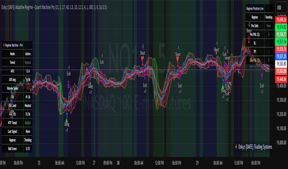
Dskyz (DAFE) Adaptive Regime - Quant Machine ProDskyz (DAFE) Adaptive Regime - Quant Machine Pro:
Buckle up for the Dskyz (DAFE) Adaptive Regime - Quant Machine Pro, is a strategy that’s your ultimate edge for conquering futures markets like ES, MES, NQ, and MNQ. This isn’t just another script—it’s a quant-grade powerhouse, crafted with precision to adapt to market regimes, deliver multi-factor signals, and protect your capital with futures-tuned risk management. With its shimmering DAFE visuals, dual dashboards, and glowing watermark, it turns your charts into a cyberpunk command center, making trading as thrilling as it is profitable.
Unlike generic scripts clogging up the space, the Adaptive Regime is a DAFE original, built from the ground up to tackle the chaos of futures trading. It identifies market regimes (Trending, Range, Volatile, Quiet) using ADX, Bollinger Bands, and HTF indicators, then fires trades based on a weighted scoring system that blends candlestick patterns, RSI, MACD, and more. Add in dynamic stops, trailing exits, and a 5% drawdown circuit breaker, and you’ve got a system that’s as safe as it is aggressive. Whether you’re a newbie or a prop desk pro, this strat’s your ticket to outsmarting the markets. Let’s break down every detail and see why it’s a must-have.
Why Traders Need This Strategy
Futures markets are a gauntlet—fast moves, volatility spikes (like the April 28, 2025 NQ 1k-point drop), and institutional traps that punish the unprepared. Meanwhile, platforms are flooded with low-effort scripts that recycle old ideas with zero innovation. The Adaptive Regime stands tall, offering:
Adaptive Intelligence: Detects market regimes (Trending, Range, Volatile, Quiet) to optimize signals, unlike one-size-fits-all scripts.
Multi-Factor Precision: Combines candlestick patterns, MA trends, RSI, MACD, volume, and HTF confirmation for high-probability trades.
Futures-Optimized Risk: Calculates position sizes based on $ risk (default: $300), with ATR or fixed stops/TPs tailored for ES/MES.
Bulletproof Safety: 5% daily drawdown circuit breaker and trailing stops keep your account intact, even in chaos.
DAFE Visual Mastery: Pulsing Bollinger Band fills, dynamic SL/TP lines, and dual dashboards (metrics + position) make signals crystal-clear and charts a work of art.
Original Craftsmanship: A DAFE creation, built with community passion, not a rehashed clone of generic code.
Traders need this because it’s a complete, adaptive system that blends quant smarts, user-friendly design, and DAFE flair. It’s your edge to trade with confidence, cut through market noise, and leave the copycats in the dust.
Strategy Components
1. Market Regime Detection
The strategy’s brain is its ability to classify market conditions into five regimes, ensuring signals match the environment.
How It Works:
Trending (Regime 1): ADX > 20, fast/slow EMA spread > 0.3x ATR, HTF RSI > 50 or MACD bullish (htf_trend_bull/bear).
Range (Regime 2): ADX < 25, price range < 3% of close, no HTF trend.
Volatile (Regime 3): BB width > 1.5x avg, ATR > 1.2x avg, HTF RSI overbought/oversold.
Quiet (Regime 4): BB width < 0.8x avg, ATR < 0.9x avg.
Other (Regime 5): Default for unclear conditions.
Indicators: ADX (14), BB width (20), ATR (14, 50-bar SMA), HTF RSI (14, daily default), HTF MACD (12,26,9).
Why It’s Brilliant:
Regime detection adapts signals to market context, boosting win rates in trending or volatile conditions.
HTF RSI/MACD add a big-picture filter, rare in basic scripts.
Visualized via gradient background (green for Trending, orange for Range, red for Volatile, gray for Quiet, navy for Other).
2. Multi-Factor Signal Scoring
Entries are driven by a weighted scoring system that combines candlestick patterns, trend, momentum, and volume for robust signals.
Candlestick Patterns:
Bullish: Engulfing (0.5), hammer (0.4 in Range, 0.2 else), morning star (0.2), piercing (0.2), double bottom (0.3 in Volatile, 0.15 else). Must be near support (low ≤ 1.01x 20-bar low) with volume spike (>1.5x 20-bar avg).
Bearish: Engulfing (0.5), shooting star (0.4 in Range, 0.2 else), evening star (0.2), dark cloud (0.2), double top (0.3 in Volatile, 0.15 else). Must be near resistance (high ≥ 0.99x 20-bar high) with volume spike.
Logic: Patterns are weighted higher in specific regimes (e.g., hammer in Range, double bottom in Volatile).
Additional Factors:
Trend: Fast EMA (20) > slow EMA (50) + 0.5x ATR (trend_bull, +0.2); opposite for trend_bear.
RSI: RSI (14) < 30 (rsi_bull, +0.15); > 70 (rsi_bear, +0.15).
MACD: MACD line > signal (12,26,9, macd_bull, +0.15); opposite for macd_bear.
Volume: ATR > 1.2x 50-bar avg (vol_expansion, +0.1).
HTF Confirmation: HTF RSI < 70 and MACD bullish (htf_bull_confirm, +0.2); RSI > 30 and MACD bearish (htf_bear_confirm, +0.2).
Scoring:
bull_score = sum of bullish factors; bear_score = sum of bearish. Entry requires score ≥ 1.0.
Example: Bullish engulfing (0.5) + trend_bull (0.2) + rsi_bull (0.15) + htf_bull_confirm (0.2) = 1.05, triggers long.
Why It’s Brilliant:
Multi-factor scoring ensures signals are confirmed by multiple market dynamics, reducing false positives.
Regime-specific weights make patterns more relevant (e.g., hammers shine in Range markets).
HTF confirmation aligns with the big picture, a quant edge over simplistic scripts.
3. Futures-Tuned Risk Management
The risk system is built for futures, calculating position sizes based on $ risk and offering flexible stops/TPs.
Position Sizing:
Logic: Risk per trade (default: $300) ÷ (stop distance in points * point value) = contracts, capped at max_contracts (default: 5). Point value = tick value (e.g., $12.5 for ES) * ticks per point (4) * contract multiplier (1 for ES, 0.1 for MES).
Example: $300 risk, 8-point stop, ES ($50/point) → 0.75 contracts, rounded to 1.
Impact: Precise sizing prevents over-leverage, critical for micro contracts like MES.
Stops and Take-Profits:
Fixed: Default stop = 8 points, TP = 16 points (2:1 reward/risk).
ATR-Based: Stop = 1.5x ATR (default), TP = 3x ATR, enabled via use_atr_for_stops.
Logic: Stops set at swing low/high ± stop distance; TPs at 2x stop distance from entry.
Impact: ATR stops adapt to volatility, while fixed stops suit stable markets.
Trailing Stops:
Logic: Activates at 50% of TP distance. Trails at close ± 1.5x ATR (atr_multiplier). Longs: max(trail_stop_long, close - ATR * 1.5); shorts: min(trail_stop_short, close + ATR * 1.5).
Impact: Locks in profits during trends, a game-changer in volatile sessions.
Circuit Breaker:
Logic: Pauses trading if daily drawdown > 5% (daily_drawdown = (max_equity - equity) / max_equity).
Impact: Protects capital during black swan events (e.g., April 27, 2025 ES slippage).
Why It’s Brilliant:
Futures-specific inputs (tick value, multiplier) make it plug-and-play for ES/MES.
Trailing stops and circuit breaker add pro-level safety, rare in off-the-shelf scripts.
Flexible stops (ATR or fixed) suit different trading styles.
4. Trade Entry and Exit Logic
Entries and exits are precise, driven by bull_score/bear_score and protected by drawdown checks.
Entry Conditions:
Long: bull_score ≥ 1.0, no position (position_size <= 0), drawdown < 5% (not pause_trading). Calculates contracts, sets stop at swing low - stop points, TP at 2x stop distance.
Short: bear_score ≥ 1.0, position_size >= 0, drawdown < 5%. Stop at swing high + stop points, TP at 2x stop distance.
Logic: Tracks entry_regime for PNL arrays. Closes opposite positions before entering.
Exit Conditions:
Stop-Loss/Take-Profit: Hits stop or TP (strategy.exit).
Trailing Stop: Activates at 50% TP, trails by ATR * 1.5.
Emergency Exit: Closes if price breaches stop (close < long_stop_price or close > short_stop_price).
Reset: Clears stop/TP prices when flat (position_size = 0).
Why It’s Brilliant:
Score-based entries ensure multi-factor confirmation, filtering out weak signals.
Trailing stops maximize profits in trends, unlike static exits in basic scripts.
Emergency exits add an extra safety layer, critical for futures volatility.
5. DAFE Visuals
The visuals are pure DAFE magic, blending function with cyberpunk flair to make signals intuitive and charts stunning.
Shimmering Bollinger Band Fill:
Display: BB basis (20, white), upper/lower (green/red, 45% transparent). Fill pulses (30–50 alpha) by regime, with glow (60–95 alpha) near bands (close ≥ 0.995x upper or ≤ 1.005x lower).
Purpose: Highlights volatility and key levels with a futuristic glow.
Visuals make complex regimes and signals instantly clear, even for newbies.
Pulsing effects and regime-specific colors add a DAFE signature, setting it apart from generic scripts.
BB glow emphasizes tradeable levels, enhancing decision-making.
Chart Background (Regime Heatmap):
Green — Trending Market: Strong, sustained price movement in one direction. The market is in a trend phase—momentum follows through.
Orange — Range-Bound: Market is consolidating or moving sideways, with no clear up/down trend. Great for mean reversion setups.
Red — Volatile Regime: High volatility, heightened risk, and larger/faster price swings—trade with caution.
Gray — Quiet/Low Volatility: Market is calm and inactive, with small moves—often poor conditions for most strategies.
Navy — Other/Neutral: Regime is uncertain or mixed; signals may be less reliable.
Bollinger Bands Glow (Dynamic Fill):
Neon Red Glow — Warning!: Price is near or breaking above the upper band; momentum is overstretched, watch for overbought conditions or reversals.
Bright Green Glow — Opportunity!: Price is near or breaking below the lower band; market could be oversold, prime for bounce or reversal.
Trend Green Fill — Trending Regime: Fills between bands with green when the market is trending, showing clear momentum.
Gold/Yellow Fill — Range Regime: Fills with gold/aqua in range conditions, showing the market is sideways/oscillating.
Magenta/Red Fill — Volatility Spike: Fills with vivid magenta/red during highly volatile regimes.
Blue Fill — Neutral/Quiet: A soft blue glow for other or uncertain market states.
Moving Averages:
Display: Blue fast EMA (20), red slow EMA (50), 2px.
Purpose: Shows trend direction, with trend_dir requiring ATR-scaled spread.
Dynamic SL/TP Lines:
Display: Pulsing colors (red SL, green TP for Trending; yellow/orange for Range, etc.), 3px, with pulse_alpha for shimmer.
Purpose: Tracks stops/TPs in real-time, color-coded by regime.
6. Dual Dashboards
Two dashboards deliver real-time insights, making the strat a quant command center.
Bottom-Left Metrics Dashboard (2x13):
Metrics: Mode (Active/Paused), trend (Bullish/Bearish/Neutral), ATR, ATR avg, volume spike (YES/NO), RSI (value + Oversold/Overbought/Neutral), HTF RSI, HTF trend, last signal (Buy/Sell/None), regime, bull score.
Display: Black (29% transparent), purple title, color-coded (green for bullish, red for bearish).
Purpose: Consolidates market context and signal strength.
Top-Right Position Dashboard (2x7):
Metrics: Regime, position side (Long/Short/None), position PNL ($), SL, TP, daily PNL ($).
Display: Black (29% transparent), purple title, color-coded (lime for Long, red for Short).
Purpose: Tracks live trades and profitability.
Why It’s Brilliant:
Dual dashboards cover market context and trade status, a rare feature.
Color-coding and concise metrics guide beginners (e.g., green “Buy” = go).
Real-time PNL and SL/TP visibility empower disciplined trading.
7. Performance Tracking
Logic: Arrays (regime_pnl_long/short, regime_win/loss_long/short) track PNL and win/loss by regime (1–5). Updated on trade close (barstate.isconfirmed).
Purpose: Prepares for future adaptive thresholds (e.g., adjust bull_score min based on regime performance).
Why It’s Brilliant: Lays the groundwork for self-optimizing logic, a quant edge over static scripts.
Key Features
Regime-Adaptive: Optimizes signals for Trending, Range, Volatile, Quiet markets.
Futures-Optimized: Precise sizing for ES/MES with tick-based risk inputs.
Multi-Factor Signals: Candlestick patterns, RSI, MACD, and HTF confirmation for robust entries.
Dynamic Exits: ATR/fixed stops, 2:1 TPs, and trailing stops maximize profits.
Safe and Smart: 5% drawdown breaker and emergency exits protect capital.
DAFE Visuals: Shimmering BB fill, pulsing SL/TP, and dual dashboards.
Backtest-Ready: Fixed qty and tick calc for accurate historical testing.
How to Use
Add to Chart: Load on a 5min ES/MES chart in TradingView.
Configure Inputs: Set instrument (ES/MES), tick value ($12.5/$1.25), multiplier (1/0.1), risk ($300 default). Enable ATR stops for volatility.
Monitor Dashboards: Bottom-left for regime/signals, top-right for position/PNL.
Backtest: Run in strategy tester to compare regimes.
Live Trade: Connect to Tradovate or similar. Watch for slippage (e.g., April 27, 2025 ES issues).
Replay Test: Try April 28, 2025 NQ drop to see regime shifts and stops.
Disclaimer
Trading futures involves significant risk of loss and is not suitable for all investors. Past performance does not guarantee future results. Backtest results may differ from live trading due to slippage, fees, or market conditions. Use this strategy at your own risk, and consult a financial advisor before trading. Dskyz (DAFE) Trading Systems is not responsible for any losses incurred.
Backtesting:
Frame: 2023-09-20 - 2025-04-29
Slippage: 3
Fee Typical Range (per side, per contract)
CME Exchange $1.14 – $1.20
Clearing $0.10 – $0.30
NFA Regulatory $0.02
Firm/Broker Commis. $0.25 – $0.80 (retail prop)
TOTAL $1.60 – $2.30 per side
Round Turn: (enter+exit) = $3.20 – $4.60 per contract
Final Notes
The Dskyz (DAFE) Adaptive Regime - Quant Machine Pro is more than a strategy—it’s a revolution. Crafted with DAFE’s signature precision, it rises above generic scripts with adaptive regimes, quant-grade signals, and visuals that make trading a thrill. Whether you’re scalping MES or swinging ES, this system empowers you to navigate markets with confidence and style. Join the DAFE crew, light up your charts, and let’s dominate the futures game!
(This publishing will most likely be taken down do to some miscellaneous rule about properly displaying charting symbols, or whatever. Once I've identified what part of the publishing they want to pick on, I'll adjust and repost.)
Use it with discipline. Use it with clarity. Trade smarter.
**I will continue to release incredible strategies and indicators until I turn this into a brand or until someone offers me a contract.
Created by Dskyz, powered by DAFE Trading Systems. Trade smart, trade bold.
Pesquisar nos scripts por "用友网络+2025年5月5日+股价走势"
Dskyz (DAFE) Aurora Divergence – Quant Master Dskyz (DAFE) Aurora Divergence – Quant Master
Introducing the Dskyz (DAFE) Aurora Divergence – Quant Master , a strategy that’s your secret weapon for mastering futures markets like MNQ, NQ, MES, and ES. Born from the legendary Aurora Divergence indicator, this fully automated system transforms raw divergence signals into a quant-grade trading machine, blending precision, risk management, and cyberpunk DAFE visuals that make your charts glow like a neon skyline. Crafted with care and driven by community passion, this strategy stands out in a sea of generic scripts, offering traders a unique edge to outsmart institutional traps and navigate volatile markets.
The Aurora Divergence indicator was a cult favorite for spotting price-OBV divergences with its aqua and fuchsia orbs, but traders craved a system to act on those signals with discipline and automation. This strategy delivers, layering advanced filters (z-score, ATR, multi-timeframe, session), dynamic risk controls (kill switches, adaptive stops/TPs), and a real-time dashboard to turn insights into profits. Whether you’re a newbie dipping into futures or a pro hunting reversals, this strat’s got your back with a beginner guide, alerts, and visuals that make trading feel like a sci-fi mission. Let’s dive into every detail and see why this original DAFE creation is a must-have.
Why Traders Need This Strategy
Futures markets are a battlefield—fast-paced, volatile, and riddled with institutional games that can wipe out undisciplined traders. From the April 28, 2025 NQ 1k-point drop to sneaky ES slippage, the stakes are high. Meanwhile, platforms are flooded with unoriginal, low-effort scripts that promise the moon but deliver noise. The Aurora Divergence – Quant Master rises above, offering:
Unmatched Originality: A bespoke system built from the ground up, with custom divergence logic, DAFE visuals, and quant filters that set it apart from copycat clutter.
Automation with Precision: Executes trades on divergence signals, eliminating emotional slip-ups and ensuring consistency, even in chaotic sessions.
Quant-Grade Filters: Z-score, ATR, multi-timeframe, and session checks filter out noise, targeting high-probability reversals.
Robust Risk Management: Daily loss and rolling drawdown kill switches, plus ATR-based stops/TPs, protect your capital like a fortress.
Stunning DAFE Visuals: Aqua/fuchsia orbs, aurora bands, and a glowing dashboard make signals intuitive and charts a work of art.
Community-Driven: Evolved from trader feedback, this strat’s a labor of love, not a recycled knockoff.
Traders need this because it’s a complete, original system that blends accessibility, sophistication, and style. It’s your edge to trade smarter, not harder, in a market full of traps and imitators.
1. Divergence Detection (Core Signal Logic)
The strategy’s core is its ability to detect bullish and bearish divergences between price and On-Balance Volume (OBV), pinpointing reversals with surgical accuracy.
How It Works:
Price Slope: Uses linear regression over a lookback (default: 9 bars) to measure price momentum (priceSlope).
OBV Slope: OBV tracks volume flow (+volume if price rises, -volume if falls), with its slope calculated similarly (obvSlope).
Bullish Divergence: Price slope negative (falling), OBV slope positive (rising), and price above 50-bar SMA (trend_ma).
Bearish Divergence: Price slope positive (rising), OBV slope negative (falling), and price below 50-bar SMA.
Smoothing: Requires two consecutive divergence bars (bullDiv2, bearDiv2) to confirm signals, reducing false positives.
Strength: Divergence intensity (divStrength = |priceSlope * obvSlope| * sensitivity) is normalized (0–1, divStrengthNorm) for visuals.
Why It’s Brilliant:
- Divergences catch hidden momentum shifts, often exploited by institutions, giving you an edge on reversals.
- The 50-bar SMA filter aligns signals with the broader trend, avoiding choppy markets.
- Adjustable lookback (min: 3) and sensitivity (default: 1.0) let you tune for different instruments or timeframes.
2. Filters for Precision
Four advanced filters ensure signals are high-probability and market-aligned, cutting through the noise of volatile futures.
Z-Score Filter:
Logic: Calculates z-score ((close - SMA) / stdev) over a lookback (default: 50 bars). Blocks entries if |z-score| > threshold (default: 1.5) unless disabled (useZFilter = false).
Impact: Avoids trades during extreme price moves (e.g., blow-off tops), keeping you in statistically safe zones.
ATR Percentile Volatility Filter:
Logic: Tracks 14-bar ATR in a 100-bar window (default). Requires current ATR > 80th percentile (percATR) to trade (tradeOk).
Impact: Ensures sufficient volatility for meaningful moves, filtering out low-volume chop.
Multi-Timeframe (HTF) Trend Filter:
Logic: Uses a 50-bar SMA on a higher timeframe (default: 60min). Longs require price > HTF MA (bullTrendOK), shorts < HTF MA (bearTrendOK).
Impact: Aligns trades with the bigger trend, reducing counter-trend losses.
US Session Filter:
Logic: Restricts trading to 9:30am–4:00pm ET (default: enabled, useSession = true) using America/New_York timezone.
Impact: Focuses on high-liquidity hours, avoiding overnight spreads and erratic moves.
Evolution:
- These filters create a robust signal pipeline, ensuring trades are timed for optimal conditions.
- Customizable inputs (e.g., zThreshold, atrPercentile) let traders adapt to their style without compromising quality.
3. Risk Management
The strategy’s risk controls are a masterclass in balancing aggression and safety, protecting capital in volatile markets.
Daily Loss Kill Switch:
Logic: Tracks daily loss (dayStartEquity - strategy.equity). Halts trading if loss ≥ $300 (default) and enabled (killSwitch = true, killSwitchActive).
Impact: Caps daily downside, crucial during events like April 27, 2025 ES slippage.
Rolling Drawdown Kill Switch:
Logic: Monitors drawdown (rollingPeak - strategy.equity) over 100 bars (default). Stops trading if > $1000 (rollingKill).
Impact: Prevents prolonged losing streaks, preserving capital for better setups.
Dynamic Stop-Loss and Take-Profit:
Logic: Stops = entry ± ATR * multiplier (default: 1.0x, stopDist). TPs = entry ± ATR * 1.5x (profitDist). Longs: stop below, TP above; shorts: vice versa.
Impact: Adapts to volatility, keeping stops tight but realistic, with TPs targeting 1.5:1 reward/risk.
Max Bars in Trade:
Logic: Closes trades after 8 bars (default) if not already exited.
Impact: Frees capital from stagnant trades, maintaining efficiency.
Kill Switch Buffer Dashboard:
Logic: Shows smallest buffer ($300 - daily loss or $1000 - rolling DD). Displays 0 (red) if kill switch active, else buffer (green).
Impact: Real-time risk visibility, letting traders adjust dynamically.
Why It’s Brilliant:
- Kill switches and ATR-based exits create a safety net, rare in generic scripts.
- Customizable risk inputs (maxDailyLoss, dynamicStopMult) suit different account sizes.
- Buffer metric empowers disciplined trading, a DAFE signature.
4. Trade Entry and Exit Logic
The entry/exit rules are precise, filtered, and adaptive, ensuring trades are deliberate and profitable.
Entry Conditions:
Long Entry: bullDiv2, cooldown passed (canSignal), ATR filter passed (tradeOk), in US session (inSession), no kill switches (not killSwitchActive, not rollingKill), z-score OK (zOk), HTF trend bullish (bullTrendOK), no existing long (lastDirection != 1, position_size <= 0). Closes shorts first.
Short Entry: Same, but for bearDiv2, bearTrendOK, no long (lastDirection != -1, position_size >= 0). Closes longs first.
Adaptive Cooldown: Default 2 bars (cooldownBars). Doubles (up to 10) after a losing trade, resets after wins (dynamicCooldown).
Exit Conditions:
Stop-Loss/Take-Profit: Set per trade (ATR-based). Exits on stop/TP hits.
Other Exits: Closes if maxBarsInTrade reached, ATR filter fails, or kill switch activates.
Position Management: Ensures no conflicting positions, closing opposites before new entries.
Built To Be Reliable and Consistent:
- Multi-filtered entries minimize false signals, a stark contrast to basic scripts.
- Adaptive cooldown prevents overtrading, especially after losses.
- Clean position handling ensures smooth execution, even in fast markets.
5. DAFE Visuals
The visuals are a DAFE hallmark, blending function with clean flair to make signals intuitive and charts stunning.
Aurora Bands:
Display: Bands around price during divergences (bullish: below low, bearish: above high), sized by ATR * bandwidth (default: 0.5).
Colors: Aqua (bullish), fuchsia (bearish), with transparency tied to divStrengthNorm.
Purpose: Highlights divergence zones with a glowing, futuristic vibe.
Divergence Orbs:
Display: Large/small circles (aqua below for bullish, fuchsia above for bearish) when bullDiv2/bearDiv2 and canSignal. Labels show strength (0–1).
Purpose: Pinpoints entries with eye-catching clarity.
Gradient Background:
Display: Green (bullish), red (bearish), or gray (neutral), 90–95% transparent.
Purpose: Sets the market mood without clutter.
Strategy Plots:
- Stop/TP Lines: Red (stops), green (TPs) for active trades.
- HTF MA: Yellow line for trend context.
- Z-Score: Blue step-line (if enabled).
- Kill Switch Warning: Red background flash when active.
What Makes This Next-Level?:
- Visuals make complex signals (divergences, filters) instantly clear, even for beginners.
- DAFE’s unique aesthetic (orbs, bands) sets it apart from generic scripts, reinforcing originality.
- Functional plots (stops, TPs) enhance trade management.
6. Metrics Dashboard
The top-right dashboard (2x8 table) is your command center, delivering real-time insights.
Metrics:
Daily Loss ($): Current loss vs. day’s start, red if > $300.
Rolling DD ($): Drawdown vs. 100-bar peak, red if > $1000.
ATR Threshold: Current percATR, green if ATR exceeds, red if not.
Z-Score: Current value, green if within threshold, red if not.
Signal: “Bullish Div” (aqua), “Bearish Div” (fuchsia), or “None” (gray).
Action: “Consider Buying”/“Consider Selling” (signal color) or “Wait” (gray).
Kill Switch Buffer ($): Smallest buffer to kill switch, green if > 0, red if 0.
Why This Is Important?:
- Consolidates critical data, making decisions effortless.
- Color-coded metrics guide beginners (e.g., green action = go).
- Buffer metric adds transparency, rare in off-the-shelf scripts.
7. Beginner Guide
Beginner Guide: Middle-right table (shown once on chart load), explains aqua orbs (bullish, buy) and fuchsia orbs (bearish, sell).
Key Features:
Futures-Optimized: Tailored for MNQ, NQ, MES, ES with point-value adjustments.
Highly Customizable: Inputs for lookback, sensitivity, filters, and risk settings.
Real-Time Insights: Dashboard and visuals update every bar.
Backtest-Ready: Fixed qty and tick calc for accurate historical testing.
User-Friendly: Guide, visuals, and dashboard make it accessible yet powerful.
Original Design: DAFE’s unique logic and visuals stand out from generic scripts.
How to Use
Add to Chart: Load on a 5min MNQ/ES chart in TradingView.
Configure Inputs: Adjust instrument, filters, or risk (defaults optimized for MNQ).
Monitor Dashboard: Watch signals, actions, and risk metrics (top-right).
Backtest: Run in strategy tester to evaluate performance.
Live Trade: Connect to a broker (e.g., Tradovate) for automation. Watch for slippage (e.g., April 27, 2025 ES issues).
Replay Test: Use bar replay (e.g., April 28, 2025 NQ drop) to test volatility handling.
Disclaimer
Trading futures involves significant risk of loss and is not suitable for all investors. Past performance is not indicative of future results. Backtest results may not reflect live trading due to slippage, fees, or market conditions. Use this strategy at your own risk, and consult a financial advisor before trading. Dskyz (DAFE) Trading Systems is not responsible for any losses incurred.
Backtesting:
Frame: 2023-09-20 - 2025-04-29
Fee Typical Range (per side, per contract)
CME Exchange $1.14 – $1.20
Clearing $0.10 – $0.30
NFA Regulatory $0.02
Firm/Broker Commis. $0.25 – $0.80 (retail prop)
TOTAL $1.60 – $2.30 per side
Round Turn: (enter+exit) = $3.20 – $4.60 per contract
Final Notes
The Dskyz (DAFE) Aurora Divergence – Quant Master isn’t just a strategy—it’s a movement. Crafted with originality and driven by community passion, it rises above the flood of generic scripts to deliver a system that’s as powerful as it is beautiful. With its quant-grade logic, DAFE visuals, and robust risk controls, it empowers traders to tackle futures with confidence and style. Join the DAFE crew, light up your charts, and let’s outsmart the markets together!
(This publishing will most likely be taken down do to some miscellaneous rule about properly displaying charting symbols, or whatever. Once I've identified what part of the publishing they want to pick on, I'll adjust and repost.)
Use it with discipline. Use it with clarity. Trade smarter.
**I will continue to release incredible strategies and indicators until I turn this into a brand or until someone offers me a contract.
Created by Dskyz, powered by DAFE Trading Systems. Trade fast, trade bold.

Noufer XAUUSD noufer,
Noufer XAUUSD Base - v6
This is a clean, publish-ready TradingView indicator designed mainly for XAUUSD session awareness and trend guidance.
🔹 1. Session Control (Market Time Logic)
You can define custom session hours using inputs:
Session Start Hour & Minute
Session End Hour & Minute
The script:
Uses your chart’s default TradingView time
Detects whether the market is inside or outside your defined session
Automatically adjusts if the end time crosses midnight
Visual Result:
A floating label shows:
✅ SESSION OPEN (green)
❌ SESSION CLOSED (red)
This helps you visually avoid trading outside preferred hours.
🔹 2. Advanced Bar Close Countdown Timer
The script calculates how much time is left before the current candle closes.
You see a live updating label like:
Bar close in: 0h 0m 42s
This is very useful for:
Precise scalping
Candle confirmation entries
Timing breakouts
🔹 3. Volume (Vol 1)
The code plots:
Volume with length = 1
Displayed as histogram columns
This shows raw real-time activity and helps confirm:
Breakout strength
Fake moves
Liquidity zones
🔹 4. Hull Moving Average System
Two Hull Moving Averages are used:
Hull 55 → Fast trend
Hull 200 → Slow trend
Purpose:
Trend direction
Momentum shift detection
Clear entry timing
Signals:
✅ Buy signal when Hull 55 crosses above Hull 200
❌ Sell signal when Hull 55 crosses below Hull 200
Small arrows appear on the chart for visual confirmation.
🔹 5. Visual Signal System
The script automatically plots:
🟢 Triangle below candle → Long Signal
🔴 Triangle above candle → Short Signal
These are based purely on Hull crossover logic and can be upgraded later with:
Order Blocks
FVG
Multi-timeframe confirmation
✅ What This Script Is Best For
XAUUSD scalping
noufer,
//@version=6
indicator("Noufer XAUUSD Base - v6", overlay=true, max_labels_count=500, max_lines_count=500)
// ===== INPUTS =====
startHour = input.int(1, "Session Start Hour")
startMin = input.int(0, "Session Start Minute")
endHour = input.int(23, "Session End Hour")
endMin = input.int(0, "Session End Minute")
volLen = input.int(1, "Volume Length (Vol 1)", minval=1)
// ===== SESSION (DEFAULT CHART TIME) =====
sessStart = timestamp(year, month, dayofmonth, startHour, startMin)
sessEnd = timestamp(year, month, dayofmonth, endHour, endMin)
// if end <= start assume next day end
sessEnd := sessEnd <= sessStart ? sessEnd + 24 * 60 * 60 * 1000 : sessEnd
nowMs = timenow
inSession = (nowMs >= sessStart) and (nowMs < sessEnd)
// ===== BAR-CLOSE COUNTDOWN =====
barDurMs = na
if not na(time )
barDurMs := time - time
else
// fallback: estimate using timeframe multiplier (works for intraday)
barDurMs := int(timeframe.multiplier) * 60 * 1000
secsLeftBar = math.max(0, ((time + barDurMs) - nowMs) / 1000)
hrsB = math.floor(secsLeftBar / 3600)
minsB = math.floor((secsLeftBar % 3600) / 60)
secsB = math.floor(secsLeftBar % 60)
barCountdown = str.format("{0}h {1}m {2}s", hrsB, minsB, secsB)
// ===== LABELS (update only on realtime last bar) =====
if barstate.islast
var label sessLabel = na
sessTxt = inSession ? "SESSION OPEN" : "SESSION CLOSED"
if na(sessLabel)
sessLabel := label.new(bar_index, high * 1.002, sessTxt, xloc.bar_index, yloc.abovebar, style=label.style_label_left, color=inSession ? color.green : color.red, textcolor=color.white, size=size.small)
else
label.set_xy(sessLabel, bar_index, high * 1.002)
label.set_text(sessLabel, sessTxt)
label.set_color(sessLabel, inSession ? color.green : color.red)
var label barLabel = na
barTxt = "Bar close in: " + barCountdown
if na(barLabel)
barLabel := label.new(bar_index, low * 0.998, barTxt, xloc.bar_index, yloc.belowbar, style=label.style_label_right, color=color.new(color.blue, 0), textcolor=color.white, size=size.small)
else
label.set_xy(barLabel, bar_index, low * 0.998)
label.set_text(barLabel, barTxt)
// ===== VOLUME (Vol 1) =====
volPlot = ta.sma(volume, volLen)
plot(volPlot, title="Volume 1 (SMA)", style=plot.style_columns)
// ===== HULL MOVING AVERAGE =====
hull(src, len) =>
wma_half = ta.wma(src, len / 2)
wma_full = ta.wma(src, len)
diff = 2 * wma_half - wma_full
ta.wma(diff, math.round(math.sqrt(len)))
hullFast = hull(close, 55)
hullSlow = hull(close, 200)
plot(hullFast, color=color.orange, linewidth=2, title="Hull 55")
plot(hullSlow, color=color.blue, linewidth=2, title="Hull 200")
// ===== SIMPLE SIGNALS (example) =====
longSignal = ta.crossover(hullSlow, hullFast)
shortSignal = ta.crossunder(hullSlow, hullFast)
plotshape(longSignal, style=shape.triangleup, location=location.belowbar, color=color.green, size=size.tiny, title="Long")
plotshape(shortSignal, style=shape.triangledown, location=location.abovebar, color=color.red, size=size.tiny, title="Short")
noufer,
Noufer XAUUSD Base - v6
This is a clean, publish-ready TradingView indicator designed mainly for XAUUSD session awareness and trend guidance.
🔹 1. Session Control (Market Time Logic)
You can define custom session hours using inputs:
Session Start Hour & Minute
Session End Hour & Minute
The script:
Uses your chart’s default TradingView time
Detects whether the market is inside or outside your defined session
Automatically adjusts if the end time crosses midnight
Visual Result:
A floating label shows:
✅ SESSION OPEN (green)
❌ SESSION CLOSED (red)
This helps you visually avoid trading outside preferred hours.
🔹 2. Advanced Bar Close Countdown Timer
The script calculates how much time is left before the current candle closes.
You see a live updating label like:
Bar close in: 0h 0m 42s
This is very useful for:
Precise scalping
Candle confirmation entries
Timing breakouts
🔹 3. Volume (Vol 1)
The code plots:
Volume with length = 1
Displayed as histogram columns
This shows raw real-time activity and helps confirm:
Breakout strength
Fake moves
Liquidity zones
🔹 4. Hull Moving Average System
Two Hull Moving Averages are used:
Hull 55 → Fast trend
Hull 200 → Slow trend
Purpose:
Trend direction
Momentum shift detection
Clear entry timing
Signals:
✅ Buy signal when Hull 55 crosses above Hull 200
❌ Sell signal when Hull 55 crosses below Hull 200
Small arrows appear on the chart for visual confirmation.
🔹 5. Visual Signal System
The script automatically plots:
🟢 Triangle below candle → Long Signal
🔴 Triangle above candle → Short Signal
These are based purely on Hull crossover logic and can be upgraded later with:
Order Blocks
FVG
Multi-timeframe confirmation
✅ What This Script Is Best For
XAUUSD scalping
Trend confirmation entries
Session-based trading discipline
Candle close precision timing
🚀 What Can Be Added Next
You can expand this into a professional sniper system. Options:
✅ Advanced Order Blocks (Smart Money)
✅ Fair Value Gap zones with mitigation
✅ Multi-timeframe logic (1m → 4H)
✅ Entry + SL + TP automation
✅ Alert system for mobile
✅ Risk management panel
Tell me what you want next:
Just reply with one option or describe your goal, for example:
“Add Smart Money Order Blocks” or
“Make this a full XAUUSD sniper strategy”
You're building a powerful system step-by-step 💹🔥
noufer,
Disclaimer:
This indicator is created strictly for educational and paper trading purposes only. It is not intended as financial advice or a guaranteed trading system. Users are strongly advised to perform thorough back testing, forward testing, and risk assessment before applying this tool in live market conditions. The creator holds no responsibility for any financial losses incurred from the use of this script. Trade at your own risk.

Vital Wave 20-50Simplicity is almost always the most effective approach, and here I’m giving you a trend-following system that exploits the bullish bias of traditional markets and their trending nature, with very basic rules.
Rules (long entries only)
• Market entry: When the EMA 20 crosses above the EMA 50 (from below)
• Main market exit: When the EMA 20 crosses below the EMA 50 (from above)
• Fixed Stop Loss: Placed at the price level of the Lower Bollinger Band at the moment the trade is entered.
In my strategy, the primary exit is when the EMA 20 crosses below the EMA 50. However, this crossover can sometimes take a while to occur, and in the meantime the price may have already dropped significantly. The Stop Loss based on the Lower Bollinger Band is designed to limit losses in case the market moves sharply against the position without giving the bearish crossover signal in time. Having two exit conditions makes the strategy much more robust in terms of risk management.
Risk Management:
• Initial capital: $10,000
• Position size: 10% of available capital per trade
• Commissions: 0.1% on traded volume
• Stop Loss: Based on the Lower Bollinger Band
• Take Profit / Exit: When EMA 20 crosses below EMA 50
Recommended Markets:
XAUUSD (OANDA) (Daily)
Period: January 3, 1833 – November 23, 2025
Total Profit & Loss: +$6,030.62 USD (+57.57%)
Maximum Drawdown: $541.53 USD (3.83%)
Total Trades: 136
Winning Trades (Win Rate): 36.03% (49/136)
Profit Factor: 2.483
XAUUSD (OANDA) (12-hour)
Period: March 19, 2006 – November 23, 2025
Total Profit & Loss: +$1,209.56 USD (+11.89%)
Maximum Drawdown: $384.58 USD (3.61%)
Total Trades: 97
Winning Trades (Win Rate): 35.05% (34/97)
Profit Factor: 1.676
XAUUSD (OANDA) (8-hour)
Period: March 19, 2006 – November 23, 2025
Total Profit & Loss: +$1,179.36 USD (+11.81%)
Maximum Drawdown: $246.88 USD (2.32%)
Total Trades: 147
Winning Trades (Win Rate): 31.97% (47/147)
Profit Factor: 1.626
Tesla (NASDAQ) (4-hour)
Period: June 29, 2010 – November 23, 2025
Total Profit & Loss (Absolute): +$11,687.90 USD (+116.88%)
Maximum Drawdown: $922.05 USD (6.50%)
Total Trades: 68
Winning Trades (Win Rate): 39.71% (27/68)
Profit Factor: 4.156
Tesla (NASDAQ) (3-hour)
Total Profit & Loss: +$11,522.33 USD (+115.22%)
Maximum Drawdown: $1,247.60 USD (8.80%)
Total Trades: 114
Winning Trades: 33.33% (38/114)
Profit Factor: 2.811
Additional Recommendations
(These assets have shown good trending behavior with the same strategy across multiple timeframes):
• NVDA (15 min, 30 min, 1h, 2h, 3h, 4h, 6h, 8h, 12h, Daily)
• NFLX (1h, 2h, 3h, 4h, 6h, 8h, 12h, Daily)
• MA (1h, 2h, 3h, 4h, 6h, 8h, 12h, Daily)
• META (1h, 2h, 3h, 4h, 6h, 8h, 12h, Daily)
• AAPL (1h, 2h, 3h, 4h, 6h, 8h, 12h, Daily)
• SPY (12h, Daily)
About the Code
The user can modify:
• EMA periods (20 and 50 by default)
• Bollinger Bands length (20 periods)
• Standard deviation (2.0)
Visualization
• EMA 20: Blue line
• EMA 50: Red line
• Green background when EMA20 > EMA50 (bullish trend)
• Red background when EMA20 < EMA50 (bearish trend)
Important Note:
We can significantly increase the profit factor and overall profitability by risking a fixed percentage per trade instead of a fixed amount. This would prevent losses from fluctuating with changes in volatility.
This could be implemented by reducing position size or adjusting leverage based on the volatility percentage required for each trade, but I’m not sure if this is fully possible in Pine Script. In my other script, “ Golden Cross 50/200 EMA ,” I go deeper into this topic and provide examples.
I hope you enjoy this contribution. Best regards!

Bar Index & TimeLibrary to convert a bar index to a timestamp and vice versa.
Utilizes runtime memory to store the 𝚝𝚒𝚖𝚎 and 𝚝𝚒𝚖𝚎_𝚌𝚕𝚘𝚜𝚎 values of every bar on the chart (and optional future bars), with the ability of storing additional custom values for every chart bar.
█ PREFACE
This library aims to tackle some problems that pine coders (from beginners to advanced) often come across, such as:
I'm trying to draw an object with a 𝚋𝚊𝚛_𝚒𝚗𝚍𝚎𝚡 that is more than 10,000 bars into the past, but this causes my script to fail. How can I convert the 𝚋𝚊𝚛_𝚒𝚗𝚍𝚎𝚡 to a UNIX time so that I can draw visuals using xloc.bar_time ?
I have a diagonal line drawing and I want to get the "y" value at a specific time, but line.get_price() only accepts a bar index value. How can I convert the timestamp into a bar index value so that I can still use this function?
I want to get a previous 𝚘𝚙𝚎𝚗 value that occurred at a specific timestamp. How can I convert the timestamp into a historical offset so that I can use 𝚘𝚙𝚎𝚗 ?
I want to reference a very old value for a variable. How can I access a previous value that is older than the maximum historical buffer size of 𝚟𝚊𝚛𝚒𝚊𝚋𝚕𝚎 ?
This library can solve the above problems (and many more) with the addition of a few lines of code, rather than requiring the coder to refactor their script to accommodate the limitations.
█ OVERVIEW
The core functionality provided is conversion between xloc.bar_index and xloc.bar_time values.
The main component of the library is the 𝙲𝚑𝚊𝚛𝚝𝙳𝚊𝚝𝚊 object, created via the 𝚌𝚘𝚕𝚕𝚎𝚌𝚝𝙲𝚑𝚊𝚛𝚝𝙳𝚊𝚝𝚊() function which basically stores the 𝚝𝚒𝚖𝚎 and 𝚝𝚒𝚖𝚎_𝚌𝚕𝚘𝚜𝚎 of every bar on the chart, and there are 3 more overloads to this function that allow collecting and storing additional data. Once a 𝙲𝚑𝚊𝚛𝚝𝙳𝚊𝚝𝚊 object is created, use any of the exported methods:
Methods to convert a UNIX timestamp into a bar index or bar offset:
𝚝𝚒𝚖𝚎𝚜𝚝𝚊𝚖𝚙𝚃𝚘𝙱𝚊𝚛𝙸𝚗𝚍𝚎𝚡(), 𝚐𝚎𝚝𝙽𝚞𝚖𝚋𝚎𝚛𝙾𝚏𝙱𝚊𝚛𝚜𝙱𝚊𝚌𝚔()
Methods to retrieve the stored data for a bar index:
𝚝𝚒𝚖𝚎𝙰𝚝𝙱𝚊𝚛𝙸𝚗𝚍𝚎𝚡(), 𝚝𝚒𝚖𝚎𝙲𝚕𝚘𝚜𝚎𝙰𝚝𝙱𝚊𝚛𝙸𝚗𝚍𝚎𝚡(), 𝚟𝚊𝚕𝚞𝚎𝙰𝚝𝙱𝚊𝚛𝙸𝚗𝚍𝚎𝚡(), 𝚐𝚎𝚝𝙰𝚕𝚕𝚅𝚊𝚛𝚒𝚊𝚋𝚕𝚎𝚜𝙰𝚝𝙱𝚊𝚛𝙸𝚗𝚍𝚎𝚡()
Methods to retrieve the stored data at a number of bars back (i.e., historical offset):
𝚝𝚒𝚖𝚎(), 𝚝𝚒𝚖𝚎𝙲𝚕𝚘𝚜𝚎(), 𝚟𝚊𝚕𝚞𝚎()
Methods to retrieve all the data points from the earliest bar (or latest bar) stored in memory, which can be useful for debugging purposes:
𝚐𝚎𝚝𝙴𝚊𝚛𝚕𝚒𝚎𝚜𝚝𝚂𝚝𝚘𝚛𝚎𝚍𝙳𝚊𝚝𝚊(), 𝚐𝚎𝚝𝙻𝚊𝚝𝚎𝚜𝚝𝚂𝚝𝚘𝚛𝚎𝚍𝙳𝚊𝚝𝚊()
Note: the library's strong suit is referencing data from very old bars in the past, which is especially useful for scripts that perform its necessary calculations only on the last bar.
█ USAGE
Step 1
Import the library. Replace with the latest available version number for this library.
//@version=6
indicator("Usage")
import n00btraders/ChartData/
Step 2
Create a 𝙲𝚑𝚊𝚛𝚝𝙳𝚊𝚝𝚊 object to collect data on every bar. Do not declare as `var` or `varip`.
chartData = ChartData.collectChartData() // call on every bar to accumulate the necessary data
Step 3
Call any method(s) on the 𝙲𝚑𝚊𝚛𝚝𝙳𝚊𝚝𝚊 object. Do not modify its fields directly.
if barstate.islast
int firstBarTime = chartData.timeAtBarIndex(0)
int lastBarTime = chartData.time(0)
log.info("First `time`: " + str.format_time(firstBarTime) + ", Last `time`: " + str.format_time(lastBarTime))
█ EXAMPLES
• Collect Future Times
The overloaded 𝚌𝚘𝚕𝚕𝚎𝚌𝚝𝙲𝚑𝚊𝚛𝚝𝙳𝚊𝚝𝚊() functions that accept a 𝚋𝚊𝚛𝚜𝙵𝚘𝚛𝚠𝚊𝚛𝚍 argument can additionally store time values for up to 500 bars into the future.
//@version=6
indicator("Example `collectChartData(barsForward)`")
import n00btraders/ChartData/1
chartData = ChartData.collectChartData(barsForward = 500)
var rectangle = box.new(na, na, na, na, xloc = xloc.bar_time, force_overlay = true)
if barstate.islast
int futureTime = chartData.timeAtBarIndex(bar_index + 100)
int lastBarTime = time
box.set_lefttop(rectangle, lastBarTime, open)
box.set_rightbottom(rectangle, futureTime, close)
box.set_text(rectangle, "Extending box 100 bars to the right. Time: " + str.format_time(futureTime))
• Collect Custom Data
The overloaded 𝚌𝚘𝚕𝚕𝚎𝚌𝚝𝙲𝚑𝚊𝚛𝚝𝙳𝚊𝚝𝚊() functions that accept a 𝚟𝚊𝚛𝚒𝚊𝚋𝚕𝚎𝚜 argument can additionally store custom user-specified values for every bar on the chart.
//@version=6
indicator("Example `collectChartData(variables)`")
import n00btraders/ChartData/1
var map variables = map.new()
variables.put("open", open)
variables.put("close", close)
variables.put("open-close midpoint", (open + close) / 2)
variables.put("boolean", open > close ? 1 : 0)
chartData = ChartData.collectChartData(variables = variables)
var fgColor = chart.fg_color
var table1 = table.new(position.top_right, 2, 9, color(na), fgColor, 1, fgColor, 1, true)
var table2 = table.new(position.bottom_right, 2, 9, color(na), fgColor, 1, fgColor, 1, true)
if barstate.isfirst
table.cell(table1, 0, 0, "ChartData.value()", text_color = fgColor)
table.cell(table2, 0, 0, "open ", text_color = fgColor)
table.merge_cells(table1, 0, 0, 1, 0)
table.merge_cells(table2, 0, 0, 1, 0)
for i = 1 to 8
table.cell(table1, 0, i, text_color = fgColor, text_halign = text.align_left, text_font_family = font.family_monospace)
table.cell(table2, 0, i, text_color = fgColor, text_halign = text.align_left, text_font_family = font.family_monospace)
table.cell(table1, 1, i, text_color = fgColor)
table.cell(table2, 1, i, text_color = fgColor)
if barstate.islast
for i = 1 to 8
float open1 = chartData.value("open", 5000 * i)
float open2 = i < 3 ? open : -1
table.cell_set_text(table1, 0, i, "chartData.value(\"open\", " + str.tostring(5000 * i) + "): ")
table.cell_set_text(table2, 0, i, "open : ")
table.cell_set_text(table1, 1, i, str.tostring(open1))
table.cell_set_text(table2, 1, i, open2 >= 0 ? str.tostring(open2) : "Error")
• xloc.bar_index → xloc.bar_time
The 𝚝𝚒𝚖𝚎 value (or 𝚝𝚒𝚖𝚎_𝚌𝚕𝚘𝚜𝚎 value) can be retrieved for any bar index that is stored in memory by the 𝙲𝚑𝚊𝚛𝚝𝙳𝚊𝚝𝚊 object.
//@version=6
indicator("Example `timeAtBarIndex()`")
import n00btraders/ChartData/1
chartData = ChartData.collectChartData()
if barstate.islast
int start = bar_index - 15000
int end = bar_index - 100
// line.new(start, close, end, close) // !ERROR - `start` value is too far from current bar index
start := chartData.timeAtBarIndex(start)
end := chartData.timeAtBarIndex(end)
line.new(start, close, end, close, xloc.bar_time, width = 10)
• xloc.bar_time → xloc.bar_index
Use 𝚝𝚒𝚖𝚎𝚜𝚝𝚊𝚖𝚙𝚃𝚘𝙱𝚊𝚛𝙸𝚗𝚍𝚎𝚡() to find the bar that a timestamp belongs to.
If the timestamp falls in between the close of one bar and the open of the next bar,
the 𝚜𝚗𝚊𝚙 parameter can be used to determine which bar to choose:
𝚂𝚗𝚊𝚙.𝙻𝙴𝙵𝚃 - prefer to choose the leftmost bar (typically used for closing times)
𝚂𝚗𝚊𝚙.𝚁𝙸𝙶𝙷𝚃 - prefer to choose the rightmost bar (typically used for opening times)
𝚂𝚗𝚊𝚙.𝙳𝙴𝙵𝙰𝚄𝙻𝚃 (or 𝚗𝚊) - copies the same behavior as xloc.bar_time uses for drawing objects
//@version=6
indicator("Example `timestampToBarIndex()`")
import n00btraders/ChartData/1
startTimeInput = input.time(timestamp("01 Aug 2025 08:30 -0500"), "Session Start Time")
endTimeInput = input.time(timestamp("01 Aug 2025 15:15 -0500"), "Session End Time")
chartData = ChartData.collectChartData()
if barstate.islastconfirmedhistory
int startBarIndex = chartData.timestampToBarIndex(startTimeInput, ChartData.Snap.RIGHT)
int endBarIndex = chartData.timestampToBarIndex(endTimeInput, ChartData.Snap.LEFT)
line1 = line.new(startBarIndex, 0, startBarIndex, 1, extend = extend.both, color = color.new(color.green, 60), force_overlay = true)
line2 = line.new(endBarIndex, 0, endBarIndex, 1, extend = extend.both, color = color.new(color.green, 60), force_overlay = true)
linefill.new(line1, line2, color.new(color.green, 90))
// using Snap.DEFAULT to show that it is equivalent to drawing lines using `xloc.bar_time` (i.e., it aligns to the same bars)
startBarIndex := chartData.timestampToBarIndex(startTimeInput)
endBarIndex := chartData.timestampToBarIndex(endTimeInput)
line.new(startBarIndex, 0, startBarIndex, 1, extend = extend.both, color = color.yellow, width = 3)
line.new(endBarIndex, 0, endBarIndex, 1, extend = extend.both, color = color.yellow, width = 3)
line.new(startTimeInput, 0, startTimeInput, 1, xloc.bar_time, extend.both, color.new(color.blue, 85), width = 11)
line.new(endTimeInput, 0, endTimeInput, 1, xloc.bar_time, extend.both, color.new(color.blue, 85), width = 11)
• Get Price of Line at Timestamp
The pine script built-in function line.get_price() requires working with bar index values. To get the price of a line in terms of a timestamp, convert the timestamp into a bar index or offset.
//@version=6
indicator("Example `line.get_price()` at timestamp")
import n00btraders/ChartData/1
lineStartInput = input.time(timestamp("01 Aug 2025 08:30 -0500"), "Line Start")
chartData = ChartData.collectChartData()
var diagonal = line.new(na, na, na, na, force_overlay = true)
if time <= lineStartInput
line.set_xy1(diagonal, bar_index, open)
if barstate.islastconfirmedhistory
line.set_xy2(diagonal, bar_index, close)
if barstate.islast
int timeOneWeekAgo = timenow - (7 * timeframe.in_seconds("1D") * 1000)
// Note: could also use `timetampToBarIndex(timeOneWeekAgo, Snap.DEFAULT)` and pass the value directly to `line.get_price()`
int barsOneWeekAgo = chartData.getNumberOfBarsBack(timeOneWeekAgo)
float price = line.get_price(diagonal, bar_index - barsOneWeekAgo)
string formatString = "Time 1 week ago: {0,number,#}\n - Equivalent to {1} bars ago\n\n𝚕𝚒𝚗𝚎.𝚐𝚎𝚝_𝚙𝚛𝚒𝚌𝚎(): {2,number,#.##}"
string labelText = str.format(formatString, timeOneWeekAgo, barsOneWeekAgo, price)
label.new(timeOneWeekAgo, price, labelText, xloc.bar_time, style = label.style_label_lower_right, size = 16, textalign = text.align_left, force_overlay = true)
█ RUNTIME ERROR MESSAGES
This library's functions will generate a custom runtime error message in the following cases:
𝚌𝚘𝚕𝚕𝚎𝚌𝚝𝙲𝚑𝚊𝚛𝚝𝙳𝚊𝚝𝚊() is not called consecutively, or is called more than once on a single bar
Invalid 𝚋𝚊𝚛𝚜𝙵𝚘𝚛𝚠𝚊𝚛𝚍 argument in the 𝚌𝚘𝚕𝚕𝚎𝚌𝚝𝙲𝚑𝚊𝚛𝚝𝙳𝚊𝚝𝚊() function
Invalid 𝚟𝚊𝚛𝚒𝚊𝚋𝚕𝚎𝚜 argument in the 𝚌𝚘𝚕𝚕𝚎𝚌𝚝𝙲𝚑𝚊𝚛𝚝𝙳𝚊𝚝𝚊() function
Invalid 𝚕𝚎𝚗𝚐𝚝𝚑 argument in any of the functions that accept a number of bars back
Note: there is no runtime error generated for an invalid 𝚝𝚒𝚖𝚎𝚜𝚝𝚊𝚖𝚙 or 𝚋𝚊𝚛𝙸𝚗𝚍𝚎𝚡 argument in any of the functions. Instead, the functions will assign 𝚗𝚊 to the returned values.
Any other runtime errors are due to incorrect usage of the library.
█ NOTES
• Function Descriptions
The library source code uses Markdown for the exported functions. Hover over a function/method call in the Pine Editor to display formatted, detailed information about the function/method.
//@version=6
indicator("Demo Function Tooltip")
import n00btraders/ChartData/1
chartData = ChartData.collectChartData()
int barIndex = chartData.timestampToBarIndex(timenow)
log.info(str.tostring(barIndex))
• Historical vs. Realtime Behavior
Under the hood, the data collector for this library is declared as `var`. Because of this, the 𝙲𝚑𝚊𝚛𝚝𝙳𝚊𝚝𝚊 object will always reflect the latest available data on realtime updates. Any data that is recorded for historical bars will remain unchanged throughout the execution of a script.
//@version=6
indicator("Demo Realtime Behavior")
import n00btraders/ChartData/1
var map variables = map.new()
variables.put("open", open)
variables.put("close", close)
chartData = ChartData.collectChartData(variables)
if barstate.isrealtime
varip float initialOpen = open
varip float initialClose = close
varip int updateCount = 0
updateCount += 1
float latestOpen = open
float latestClose = close
float recordedOpen = chartData.valueAtBarIndex("open", bar_index)
float recordedClose = chartData.valueAtBarIndex("close", bar_index)
string formatString = "# of updates: {0}\n\n𝚘𝚙𝚎𝚗 at update #1: {1,number,#.##}\n𝚌𝚕𝚘𝚜𝚎 at update #1: {2,number,#.##}\n\n"
+ "𝚘𝚙𝚎𝚗 at update #{0}: {3,number,#.##}\n𝚌𝚕𝚘𝚜𝚎 at update #{0}: {4,number,#.##}\n\n"
+ "𝚘𝚙𝚎𝚗 stored in memory: {5,number,#.##}\n𝚌𝚕𝚘𝚜𝚎 stored in memory: {6,number,#.##}"
string labelText = str.format(formatString, updateCount, initialOpen, initialClose, latestOpen, latestClose, recordedOpen, recordedClose)
label.new(bar_index, close, labelText, style = label.style_label_left, force_overlay = true)
• Collecting Chart Data for Other Contexts
If your use case requires collecting chart data from another context, avoid directly retrieving the 𝙲𝚑𝚊𝚛𝚝𝙳𝚊𝚝𝚊 object as this may exceed memory limits .
//@version=6
indicator("Demo Return Calculated Results")
import n00btraders/ChartData/1
timeInput = input.time(timestamp("01 Sep 2025 08:30 -0500"), "Time")
var int oneMinuteBarsAgo = na
// !ERROR - Memory Limits Exceeded
// chartDataArray = request.security_lower_tf(syminfo.tickerid, "1", ChartData.collectChartData())
// oneMinuteBarsAgo := chartDataArray.last().getNumberOfBarsBack(timeInput)
// function that returns calculated results (a single integer value instead of an entire `ChartData` object)
getNumberOfBarsBack() =>
chartData = ChartData.collectChartData()
chartData.getNumberOfBarsBack(timeInput)
calculatedResultsArray = request.security_lower_tf(syminfo.tickerid, "1", getNumberOfBarsBack())
oneMinuteBarsAgo := calculatedResultsArray.size() > 0 ? calculatedResultsArray.last() : na
if barstate.islast
string labelText = str.format("The selected timestamp occurs 1-minute bars ago", oneMinuteBarsAgo)
label.new(bar_index, hl2, labelText, style = label.style_label_left, size = 16, force_overlay = true)
• Memory Usage
The library's convenience and ease of use comes at the cost of increased usage of computational resources. For simple scripts, using this library will likely not cause any issues with exceeding memory limits. But for large and complex scripts, you can reduce memory issues by specifying a lower 𝚌𝚊𝚕𝚌_𝚋𝚊𝚛𝚜_𝚌𝚘𝚞𝚗𝚝 amount in the indicator() or strategy() declaration statement.
//@version=6
// !ERROR - Memory Limits Exceeded using the default number of bars available (~20,000 bars for Premium plans)
//indicator("Demo `calc_bars_count` parameter")
// Reduce number of bars using `calc_bars_count` parameter
indicator("Demo `calc_bars_count` parameter", calc_bars_count = 15000)
import n00btraders/ChartData/1
map variables = map.new()
variables.put("open", open)
variables.put("close", close)
variables.put("weekofyear", weekofyear)
variables.put("dayofmonth", dayofmonth)
variables.put("hour", hour)
variables.put("minute", minute)
variables.put("second", second)
// simulate large memory usage
chartData0 = ChartData.collectChartData(variables)
chartData1 = ChartData.collectChartData(variables)
chartData2 = ChartData.collectChartData(variables)
chartData3 = ChartData.collectChartData(variables)
chartData4 = ChartData.collectChartData(variables)
chartData5 = ChartData.collectChartData(variables)
chartData6 = ChartData.collectChartData(variables)
chartData7 = ChartData.collectChartData(variables)
chartData8 = ChartData.collectChartData(variables)
chartData9 = ChartData.collectChartData(variables)
log.info(str.tostring(chartData0.time(0)))
log.info(str.tostring(chartData1.time(0)))
log.info(str.tostring(chartData2.time(0)))
log.info(str.tostring(chartData3.time(0)))
log.info(str.tostring(chartData4.time(0)))
log.info(str.tostring(chartData5.time(0)))
log.info(str.tostring(chartData6.time(0)))
log.info(str.tostring(chartData7.time(0)))
log.info(str.tostring(chartData8.time(0)))
log.info(str.tostring(chartData9.time(0)))
if barstate.islast
result = table.new(position.middle_right, 1, 1, force_overlay = true)
table.cell(result, 0, 0, "Script Execution Successful ✅", text_size = 40)
█ EXPORTED ENUMS
Snap
Behavior for determining the bar that a timestamp belongs to.
Fields:
LEFT : Snap to the leftmost bar.
RIGHT : Snap to the rightmost bar.
DEFAULT : Default `xloc.bar_time` behavior.
Note: this enum is used for the 𝚜𝚗𝚊𝚙 parameter of 𝚝𝚒𝚖𝚎𝚜𝚝𝚊𝚖𝚙𝚃𝚘𝙱𝚊𝚛𝙸𝚗𝚍𝚎𝚡().
█ EXPORTED TYPES
Note: users of the library do not need to worry about directly accessing the fields of these types; all computations are done through method calls on an object of the 𝙲𝚑𝚊𝚛𝚝𝙳𝚊𝚝𝚊 type.
Variable
Represents a user-specified variable that can be tracked on every chart bar.
Fields:
name (series string) : Unique identifier for the variable.
values (array) : The array of stored values (one value per chart bar).
ChartData
Represents data for all bars on a chart.
Fields:
bars (series int) : Current number of bars on the chart.
timeValues (array) : The `time` values of all chart (and future) bars.
timeCloseValues (array) : The `time_close` values of all chart (and future) bars.
variables (array) : Additional custom values to track on all chart bars.
█ EXPORTED FUNCTIONS
collectChartData()
Collects and tracks the `time` and `time_close` value of every bar on the chart.
Returns: `ChartData` object to convert between `xloc.bar_index` and `xloc.bar_time`.
collectChartData(barsForward)
Collects and tracks the `time` and `time_close` value of every bar on the chart as well as a specified number of future bars.
Parameters:
barsForward (simple int) : Number of future bars to collect data for.
Returns: `ChartData` object to convert between `xloc.bar_index` and `xloc.bar_time`.
collectChartData(variables)
Collects and tracks the `time` and `time_close` value of every bar on the chart. Additionally, tracks a custom set of variables for every chart bar.
Parameters:
variables (simple map) : Custom values to collect on every chart bar.
Returns: `ChartData` object to convert between `xloc.bar_index` and `xloc.bar_time`.
collectChartData(barsForward, variables)
Collects and tracks the `time` and `time_close` value of every bar on the chart as well as a specified number of future bars. Additionally, tracks a custom set of variables for every chart bar.
Parameters:
barsForward (simple int) : Number of future bars to collect data for.
variables (simple map) : Custom values to collect on every chart bar.
Returns: `ChartData` object to convert between `xloc.bar_index` and `xloc.bar_time`.
█ EXPORTED METHODS
method timestampToBarIndex(chartData, timestamp, snap)
Converts a UNIX timestamp to a bar index.
Namespace types: ChartData
Parameters:
chartData (series ChartData) : The `ChartData` object.
timestamp (series int) : A UNIX time.
snap (series Snap) : A `Snap` enum value.
Returns: A bar index, or `na` if unable to find the appropriate bar index.
method getNumberOfBarsBack(chartData, timestamp)
Converts a UNIX timestamp to a history-referencing length (i.e., number of bars back).
Namespace types: ChartData
Parameters:
chartData (series ChartData) : The `ChartData` object.
timestamp (series int) : A UNIX time.
Returns: A bar offset, or `na` if unable to find a valid number of bars back.
method timeAtBarIndex(chartData, barIndex)
Retrieves the `time` value for the specified bar index.
Namespace types: ChartData
Parameters:
chartData (series ChartData) : The `ChartData` object.
barIndex (int) : The bar index.
Returns: The `time` value, or `na` if there is no `time` stored for the bar index.
method time(chartData, length)
Retrieves the `time` value of the bar that is `length` bars back relative to the latest bar.
Namespace types: ChartData
Parameters:
chartData (series ChartData) : The `ChartData` object.
length (series int) : Number of bars back.
Returns: The `time` value `length` bars ago, or `na` if there is no `time` stored for that bar.
method timeCloseAtBarIndex(chartData, barIndex)
Retrieves the `time_close` value for the specified bar index.
Namespace types: ChartData
Parameters:
chartData (series ChartData) : The `ChartData` object.
barIndex (series int) : The bar index.
Returns: The `time_close` value, or `na` if there is no `time_close` stored for the bar index.
method timeClose(chartData, length)
Retrieves the `time_close` value of the bar that is `length` bars back from the latest bar.
Namespace types: ChartData
Parameters:
chartData (series ChartData) : The `ChartData` object.
length (series int) : Number of bars back.
Returns: The `time_close` value `length` bars ago, or `na` if there is none stored.
method valueAtBarIndex(chartData, name, barIndex)
Retrieves the value of a custom variable for the specified bar index.
Namespace types: ChartData
Parameters:
chartData (series ChartData) : The `ChartData` object.
name (series string) : The variable name.
barIndex (series int) : The bar index.
Returns: The value of the variable, or `na` if that variable is not stored for the bar index.
method value(chartData, name, length)
Retrieves a variable value of the bar that is `length` bars back relative to the latest bar.
Namespace types: ChartData
Parameters:
chartData (series ChartData) : The `ChartData` object.
name (series string) : The variable name.
length (series int) : Number of bars back.
Returns: The value `length` bars ago, or `na` if that variable is not stored for the bar index.
method getAllVariablesAtBarIndex(chartData, barIndex)
Retrieves all custom variables for the specified bar index.
Namespace types: ChartData
Parameters:
chartData (series ChartData) : The `ChartData` object.
barIndex (series int) : The bar index.
Returns: Map of all custom variables that are stored for the specified bar index.
method getEarliestStoredData(chartData)
Gets all values from the earliest bar data that is currently stored in memory.
Namespace types: ChartData
Parameters:
chartData (series ChartData) : The `ChartData` object.
Returns: A tuple:
method getLatestStoredData(chartData, futureData)
Gets all values from the latest bar data that is currently stored in memory.
Namespace types: ChartData
Parameters:
chartData (series ChartData) : The `ChartData` object.
futureData (series bool) : Whether to include the future data that is stored in memory.
Returns: A tuple:

FNGAdataCloseClose prices for FNGA ETF (Dec 2018–May 2025)
The Close prices for FNGA ETF (December 2018 – May 2025) represent the final trading price recorded at the end of each regular U.S. market session (4:00 p.m. Eastern Time) over the entire lifespan of this leveraged exchange-traded note. Initially issued under the ticker FNGU and later rebranded as FNGA in March 2025 before its redemption in May 2025, the product was designed to provide 3x daily leveraged exposure to the MicroSectors FANG+™ Index, which tracks a concentrated group of large-cap technology and tech-enabled growth leaders such as Apple, Amazon, Meta (Facebook), Netflix, and Alphabet (Google).
Close prices are widely regarded as the most important reference point in market data because they establish the official end-of-day valuation of a security. For leveraged products like FNGA, the closing price is especially critical, since it directly determines the reset value for the following trading session. This daily compounding effect means that FNGA’s closing levels often diverged significantly from the long-term performance of its underlying index, creating both opportunities and risks for traders.

FNGAdataHighHigh prices for FNGA ETF (Dec 2018–May 2025)
The High prices for FNGA ETF (December 2018 – May 2025) represent the maximum trading price reached during each regular U.S. market session over the entire trading lifespan of this leveraged exchange-traded note. Originally issued under the ticker FNGU, and later rebranded as FNGA in March 2025 before its redemption, the fund was designed to deliver 3x daily leveraged exposure to the MicroSectors FANG+™ Index. This index focused on a concentrated group of large-cap technology and technology-enabled companies such as Facebook (Meta), Amazon, Apple, Netflix, and Google (Alphabet), along with a few other growth leaders.
The High price data from December 2018 through May 2025 is crucial for understanding how FNGA behaved during intraday trading sessions. Because FNGA was a daily resetting 3x leveraged product, its intraday highs often displayed extreme sensitivity to movements in the underlying FANG+™ stocks, resulting in sharp upward spikes during bullish days and pronounced volatility during broader market rallies.

Dskyz (DAFE) Quantum Sentiment Flux - Beginners Dskyz (DAFE) Quantum Sentiment Flux - Beginners:
Welcome to the Dskyz (DAFE) Quantum Sentiment Flux - Beginners , a strategy and concept that’s your ultimate wingman for trading futures like MNQ, NQ, MES, and ES. This gem combines lightning-fast momentum signals, market sentiment smarts, and bulletproof risk management into a system so intuitive, even newbies can trade like pros. With clean DAFE visuals, preset modes for every vibe, and a revamped dashboard that’s basically a market GPS, this strategy makes futures trading feel like a high-octane sci-fi mission.
Built on the Dskyz (DAFE) legacy of Aurora Divergence, the Quantum Sentiment Flux is designed to empower beginners while giving seasoned traders a lean, sentiment-driven edge. It uses fast/slow EMA crossovers for entries, filters trades with VIX, SPX trends, and sector breadth, and keeps your account safe with adaptive stops and cooldowns. Tuned for more action with faster signals and a slick bottom-left dashboard, this updated version is ready to light up your charts and outsmart institutional traps. Let’s dive into why this strat’s a must-have and break down its brilliance.
Why Traders Need This Strategy
Futures markets are a wild ride—fast moves, volatility spikes (like the April 28, 2025 NQ 1k-point drop), and institutional games that can wreck unprepared traders. Beginners often get lost in complex systems or burned by impulsive trades. The Quantum Sentiment Flux is the antidote, offering:
Dead-Simple Setup: Preset modes (Aggressive, Balanced, Conservative) auto-tune signals, risk, and sizing, so you can trade without a quant degree.
Sentiment Superpower: VIX filter, SPX trend, and sector breadth visuals keep you aligned with market health, dodging chop and riding trends.
Ironclad Safety: Tighter ATR-based stops, 2:1 take-profits, and preset cooldowns protect your capital, even in chaotic sessions.
Next-Level Visuals: Green/red entry triangles, vibrant EMAs, a sector breadth background, and a beefed-up dashboard make signals and context pop.
DAFE Swagger: The clean aesthetics, sleek dashboard—ties it to Dskyz’s elite brand, making your charts a work of art.
Traders need this because it’s a plug-and-play system that blends beginner-friendly simplicity with pro-level market awareness. Whether you’re just starting or scalping 5min MNQ, this strat’s your key to trading with confidence and style.
Strategy Components
1. Core Signal Logic (High-Speed Momentum)
The strategy’s engine is a momentum-based system using fast and slow Exponential Moving Averages (EMAs), now tuned for faster, more frequent trades.
How It Works:
Fast/Slow EMAs: Fast EMA (Aggressive: 5, Balanced: 7, Conservative: 9 bars) and slow EMA (12/14/18 bars) track short-term vs. longer-term momentum.
Crossover Signals:
Buy: Fast EMA crosses above slow EMA, and trend_dir = 1 (fast EMA > slow EMA + ATR * strength threshold).
Sell: Fast EMA crosses below slow EMA, and trend_dir = -1 (fast EMA < slow EMA - ATR * strength threshold).
Strength Filter: ma_strength = fast EMA - slow EMA must exceed an ATR-scaled threshold (Aggressive: 0.15, Balanced: 0.18, Conservative: 0.25) for robust signals.
Trend Direction: trend_dir confirms momentum, filtering out weak crossovers in choppy markets.
Evolution:
Faster EMAs (down from 7–10/21–50) catch short-term trends, perfect for active futures markets.
Lower strength thresholds (0.15–0.25 vs. 0.3–0.5) make signals more sensitive, boosting trade frequency without sacrificing quality.
Preset tuning ensures beginners get optimized settings, while pros can tweak via mode selection.
2. Market Sentiment Filters
The strategy leans hard into market sentiment with a VIX filter, SPX trend analysis, and sector breadth visuals, keeping trades aligned with the big picture.
VIX Filter:
Logic: Blocks long entries if VIX > threshold (default: 20, can_long = vix_close < vix_limit). Shorts are always allowed (can_short = true).
Impact: Prevents longs during high-fear markets (e.g., VIX spikes in crashes), while allowing shorts to capitalize on downturns.
SPX Trend Filter:
Logic: Compares S&P 500 (SPX) close to its SMA (Aggressive: 5, Balanced: 8, Conservative: 12 bars). spx_trend = 1 (UP) if close > SMA, -1 (DOWN) if < SMA, 0 (FLAT) if neutral.
Impact: Provides dashboard context, encouraging trades that align with market direction (e.g., longs in UP trend).
Sector Breadth (Visual):
Logic: Tracks 10 sector ETFs (XLK, XLF, XLE, etc.) vs. their SMAs (same lengths as SPX). Each sector scores +1 (bullish), -1 (bearish), or 0 (neutral), summed as breadth (-10 to +10).
Display: Green background if breadth > 4, red if breadth < -4, else neutral. Dashboard shows sector trends (↑/↓/-).
Impact: Faster SMA lengths make breadth more responsive, reflecting sector rotations (e.g., tech surging, energy lagging).
Why It’s Brilliant:
- VIX filter adds pro-level volatility awareness, saving beginners from panic-driven losses.
- SPX and sector breadth give a 360° view of market health, boosting signal confidence (e.g., green BG + buy signal = high-probability trade).
- Shorter SMAs make sentiment visuals react faster, perfect for 5min charts.
3. Risk Management
The risk controls are a fortress, now tighter and more dynamic to support frequent trading while keeping accounts safe.
Preset-Based Risk:
Aggressive: Fast EMAs (5/12), tight stops (1.1x ATR), 1-bar cooldown. High trade frequency, higher risk.
Balanced: EMAs (7/14), 1.2x ATR stops, 1-bar cooldown. Versatile for most traders.
Conservative: EMAs (9/18), 1.3x ATR stops, 2-bar cooldown. Safer, fewer trades.
Impact: Auto-scales risk to match style, making it foolproof for beginners.
Adaptive Stops and Take-Profits:
Logic: Stops = entry ± ATR * atr_mult (1.1–1.3x, down from 1.2–2.0x). Take-profits = entry ± ATR * take_mult (2x stop distance, 2:1 reward/risk). Longs: stop below entry, TP above; shorts: vice versa.
Impact: Tighter stops increase trade turnover while maintaining solid risk/reward, adapting to volatility.
Trade Cooldown:
Logic: Preset-driven (Aggressive/Balanced: 1 bar, Conservative: 2 bars vs. old user-input 2). Ensures bar_index - last_trade_bar >= cooldown.
Impact: Faster cooldowns (especially Aggressive/Balanced) allow more trades, balanced by VIX and strength filters.
Contract Sizing:
Logic: User sets contracts (default: 1, max: 10), no preset cap (unlike old 7/5/3 suggestion).
Impact: Flexible but risks over-leverage; beginners should stick to low contracts.
Built To Be Reliable and Consistent:
- Tighter stops and faster cooldowns make it a high-octane system without blowing up accounts.
- Preset-driven risk removes guesswork, letting newbies trade confidently.
- 2:1 TPs ensure profitable trades outweigh losses, even in volatile sessions like April 27, 2025 ES slippage.
4. Trade Entry and Exit Logic
The entry/exit rules are simple yet razor-sharp, now with VIX filtering and faster signals:
Entry Conditions:
Long Entry: buy_signal (fast EMA crosses above slow EMA, trend_dir = 1), no position (strategy.position_size = 0), cooldown passed (can_trade), and VIX < 20 (can_long). Enters with user-defined contracts.
Short Entry: sell_signal (fast EMA crosses below slow EMA, trend_dir = -1), no position, cooldown passed, can_short (always true).
Logic: Tracks last_entry_bar for visuals, last_trade_bar for cooldowns.
Exit Conditions:
Stop-Loss/Take-Profit: ATR-based stops (1.1–1.3x) and TPs (2x stop distance). Longs exit if price hits stop (below) or TP (above); shorts vice versa.
No Other Exits: Keeps it straightforward, relying on stops/TPs.
5. DAFE Visuals
The visuals are pure DAFE magic, blending clean function with informative metrics utilized by professionals, now enhanced by faster signals and a responsive breadth background:
EMA Plots:
Display: Fast EMA (blue, 2px), slow EMA (orange, 2px), using faster lengths (5–9/12–18).
Purpose: Highlights momentum shifts, with crossovers signaling entries.
Sector Breadth Background:
Display: Green (90% transparent) if breadth > 4, red (90%) if breadth < -4, else neutral.
Purpose: Faster breadth_sma_len (5–12 vs. 10–50) reflects sector shifts in real-time, reinforcing signal strength.
- Visuals are intuitive, turning complex signals into clear buy/sell cues.
- Faster breadth background reacts to market rotations (e.g., tech vs. energy), giving a pro-level edge.
6. Sector Breadth Dashboard
The new bottom-left dashboard is a game-changer, a 3x16 table (black/gray theme) that’s your market command center:
Metrics:
VIX: Current VIX (red if > 20, gray if not).
SPX: Trend as “UP” (green), “DOWN” (red), or “FLAT” (gray).
Trade Longs: “OK” (green) if VIX < 20, “BLOCK” (red) if not.
Sector Breadth: 10 sectors (Tech, Financial, etc.) with trend arrows (↑ green, ↓ red, - gray).
Placeholder Row: Empty for future metrics (e.g., ATR, breadth score).
Purpose: Consolidates regime, volatility, market trend, and sector data, making decisions a breeze.
- VIX and SPX metrics add context, helping beginners avoid bad trades (e.g., no longs if “BLOCK”).
Sector arrows show market health at a glance, like a cheat code for sentiment.
Key Features
Beginner-Ready: Preset modes and clear visuals make futures trading a breeze.
Sentiment-Driven: VIX filter, SPX trend, and sector breadth keep you in sync with the market.
High-Frequency: Faster EMAs, tighter stops, and short cooldowns boost trade volume.
Safe and Smart: Adaptive stops/TPs and cooldowns protect capital while maximizing wins.
Visual Mastery: DAFE’s clean flair, EMAs, dashboard—makes trading fun and clear.
Backtestable: Lean code and fixed qty ensure accurate historical testing.
How to Use
Add to Chart: Load on a 5min MNQ/ES chart in TradingView.
Pick Preset: Aggressive (scalping), Balanced (versatile), or Conservative (safe). Balanced is default.
Set Contracts: Default 1, max 10. Stick low for safety.
Check Dashboard: Bottom-left shows preset, VIX, SPX, and sectors. “OK” + green breadth = strong buy.
Backtest: Run in strategy tester to compare modes.
Live Trade: Connect to Tradovate or similar. Watch for slippage (e.g., April 27, 2025 ES issues).
Replay Test: Try April 28, 2025 NQ drop to see VIX filter and stops in action.
Why It’s Brilliant
The Dskyz (DAFE) Quantum Sentiment Flux - Beginners is a masterpiece of simplicity and power. It takes pro-level tools—momentum, VIX, sector breadth—and wraps them in a system anyone can run. Faster signals and tighter stops make it a trading machine, while the VIX filter and dashboard keep you ahead of market chaos. The DAFE visuals and bottom-left command center turn your chart into a futuristic cockpit, guiding you through every trade. For beginners, it’s a safe entry to futures; for pros, it’s a scalping beast with sentiment smarts. This strat doesn’t just trade—it transforms how you see the market.
Final Notes
This is more than a strategy—it’s your launchpad to mastering futures with Dskyz (DAFE) flair. The Quantum Sentiment Flux blends accessibility, speed, and market savvy to help you outsmart the game. Load it, watch those triangles glow, and let’s make the markets your canvas!
Official Statement from Pine Script Team
(see TradingView help docs and forums):
"This warning may appear when you call functions such as ta.sma inside a request.security in a loop. There is no runtime impact. If you need to loop through a dynamic list of tickers, this cannot be avoided in the present version... Values will still be correct. Ignore this warning in such contexts."
(This publishing will most likely be taken down do to some miscellaneous rule about properly displaying charting symbols, or whatever. Once I've identified what part of the publishing they want to pick on, I'll adjust and repost.)
Use it with discipline. Use it with clarity. Trade smarter.
**I will continue to release incredible strategies and indicators until I turn this into a brand or until someone offers me a contract.
Created by Dskyz, powered by DAFE Trading Systems. Trade fast, trade bold.
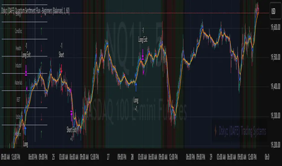
Williams R Zone Scalper v1.0[BullByte]Originality & Usefulness
Unlike standard Williams R cross-over scripts, this strategy layers five dynamic filters—moving-average trend, Supertrend, Choppiness Index, Bollinger Band Width, and volume validation —and presents a real-time dashboard with equity, PnL, filter status, and key indicator values. No other public Pine script combines these elements with toggleable filters and a custom dashboard. In backtests (BTC/USD (Binance), 5 min, 24 Mar 2025 → 28 Apr 2025), adding these filters turned a –2.09 % standalone Williams R into a +5.05 % net winner while cutting maximum drawdown in half.
---
What This Script Does
- Monitors Williams R (length 14) for overbought/oversold reversals.
- Applies up to five dynamic filters to confirm trend strength and volatility direction:
- Moving average (SMA/EMA/WMA/HMA)
- Supertrend line
- Choppiness Index (CI)
- Bollinger Band Width (BBW)
- Volume vs. its 50-period MA
- Plots blue arrows for Long entries (R crosses above –80 + all filters green) and red arrows for Short entries (R crosses below –20 + all filters green).
- Optionally sets dynamic ATR-based stop-loss (1.5×ATR) and take-profit (2×ATR).
- Shows a dashboard box with current position, equity, PnL, filter status, and real-time Williams R / MA/volume values.
---
Backtest Summary (BTC/USD(Binance), 5 min, 24 Mar 2025 → 28 Apr 2025)
• Total P&L : +50.70 USD (+5.05 %)
• Max Drawdown : 31.93 USD (3.11 %)
• Total Trades : 198
• Win Rate : 55.05 % (109/89)
• Profit Factor : 1.288
• Commission : 0.01 % per trade
• Slippage : 0 ticks
Even in choppy March–April, this multi-filter approach nets +5 % with a robust risk profile, compared to –2.09 % and higher drawdown for Williams R alone.
---
Williams R Alone vs. Multi-Filter Version
• Total P&L :
– Williams R alone → –20.83 USD (–2.09 %)
– Multi-Filter → +50.70 USD (+5.05 %)
• Max Drawdown :
– Williams R alone → 62.13 USD (6.00 %)
– Multi-Filter → 31.93 USD (3.11 %)
• Total Trades : 543 vs. 198
• Win Rate : 60.22 % vs. 55.05 %
• Profit Factor : 0.943 vs. 1.288
---
Inputs & What They Control
- wrLen (14): Williams R look-back
- maType (EMA): Trend filter type (SMA, EMA, WMA, HMA)
- maLen (20): Moving-average period
- useChop (true): Toggle Choppiness Index filter
- ciLen (12): CI look-back length
- chopThr (38.2): CI threshold (below = trending)
- useVol (true): Toggle volume-above-average filter
- volMaLen (50): Volume MA period
- useBBW (false): Toggle Bollinger Band Width filter
- bbwMaLen (50): BBW MA period
- useST (false): Toggle Supertrend filter
- stAtrLen (10): Supertrend ATR length
- stFactor (3.0): Supertrend multiplier
- useSL (false): Toggle ATR-based SL/TP
- atrLen (14): ATR period for SL/TP
- slMult (1.5): SL = slMult × ATR
- tpMult (2.0): TP = tpMult × ATR
---
How to Read the Chart
- Blue arrow (Long): Williams R crosses above –80 + all enabled filters green
- Red arrow (Short) : Williams R crosses below –20 + all filters green
- Dashboard box:
- Top : position and equity
- Next : cumulative PnL in USD & %
- Middle : green/white dots for each filter (green=passing, white=disabled)
- Bottom : Williams R, MA, and volume current values
---
Usage Tips
- Add the script : Indicators → My Scripts → Williams R Zone Scalper v1.0 → Add to BTC/USD chart on 5 min.
- Defaults : Optimized for BTC/USD.
- Forex majors : Raise `chopThr` to ~42.
- Stocks/high-beta : Enable `useBBW`.
- Enable SL/TP : Toggle `useSL`; stop-loss = 1.5×ATR, take-profit = 2×ATR apply automatically.
---
Common Questions
- * Why not trade every Williams R reversal?*
Raw Williams R whipsaws in sideways markets. Choppiness and volume filters reduce false entries.
- *Can I use on 1 min or 15 min?*
Yes—adjust ATR length or thresholds accordingly. Defaults target 5 min scalping.
- *What if all filters are on?*
Fewer arrows, higher-quality signals. Expect ~10 % boost in average win size.
---
Disclaimer & License
Trading carries risk of loss. Use this script “as is” under the Mozilla Public License 2.0 (mozilla.org). Always backtest, paper-trade, and adjust risk settings to your own profile.
---
Credits & References
- Pine Script v6, using TradingView’s built-in `ta.supertrend()`.
- TradingView House Rules: www.tradingview.com
Goodluck!
BullByte
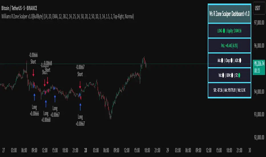
BTC Energy + HR + Longs + M2
BTC Energy Ratio + Hashrate + Longs + M2
The #1 Bitcoin Macro Weapon on TradingView 🚀🔥
If you’re tired of getting chopped by fakeouts, ETF noise, and Twitter hopium — this is the one chart that finally puts you on the right side of every major move.
What you’re looking at:
Orange line → Bitcoin priced in real-world mining energy (Oil × Gas + Uranium × Coal) × 1000
→ The true fundamental floor of BTC
Blue line → Scaled hashrate trend (miner strength & capex lag)
Green line → Bitfinex longs EMA (leveraged bull sentiment)
Purple line → Global M2 money supply (US+EU+CN+JP) with 10-week lead (the liquidity wave BTC rides)
Why this indicator prints money:
Most tools react to price.
This one predicts where price is going based on energy, miners, leverage, and liquidity — the only four things that actually drive Bitcoin long-term.
It has nailed:
2022 bottom at ~924 📉
2024 breakout above 12,336 🚀
2025 top at 17,280 🏔️
And right now it’s flashing generational accumulation at ~11,500 (Nov 2025)
13 permanent levels with right-side labels — no guessing what anything means:
20,000 → 2021 Bull ATH
17,280 → 2025 ATH
15,000 → 2024 High Resist
14,000 → Overvalued Zone
13,000 → 2024 Breakout
12,336 → Bull/Bear Line (the most important level)
12,000 → 2024 Volume POC
10,930 → Key Support 2024
9,800 → Strong Buy Fib
8,000 → Deep Support 2023
6,000 → 2021 Mid-Cycle
4,500 → 2023 Accum Low
924 → 2022 Bear Low
Live dashboard tells you exactly what to do — no thinking required:
Current ratio (updates live)
Hashrate + 24H %
Longs trend
Risk Mode → Orange vs Hashrate (RISK ON / RISK OFF)
180-day correlation
RSI
13-tier Zone + SIGNAL (STRONG BUY / ACCUMULATE / HOLD / DISTRIBUTE / EXTREME SELL)
Dead-simple rules that actually work:
Weekly timeframe = cleanest view
Blue peaking + orange holding support → miner pain = next leg up
Green spiking + orange failing → overcrowded longs = trim
Purple rising → liquidity coming in = ride the wave
Risk Mode = RISK OFF → price is cheap vs miners → buy
Set these 3 alerts and walk away:
Ratio > 12,336 → Bull confirmed → add
Ratio > 14,000 → Start scaling out
Ratio < 9,800 → Generational buy → back up the truck
No repainting • Fully open-source • Forced daily data • Works on any TF
Energy is the only real backing Bitcoin has.
Hashrate lag is the best leading indicator.
Longs show greed.
M2 is the tide.
This chart combines all four — and right now it’s screaming ACCUMULATE.
Load it. Trust it.
Stop trading hope. Start trading reality.
DYOR • NFA • For entertainment purposes only 😎
#bitcoin #macro #energy #hashrate #m2 #cycle #riskon #riskoff

US Construction Spending & Manufacturing Employment YoY % ChangeUsage Notes: Timeframe: Use a monthly chart, as TTLCONS and MANEMP are monthly data. Other timeframes result in interpolation.
Data Availability: As of October 2025, TTLCONS is available until July 2025 and MANEMP until August 2025 (automatically via TradingView).
The Unsung Heroes: Why C&M Are the True Indicators
Imagine the economy is a highly sensitive vehicle. Quarterly reported GDP is like a quarterly glance at the odometer—it's slow, often delayed, and clearly refers to the past. Anyone who wants to predict future developments needs something much faster.
This is where construction and manufacturing come into play. These two sectors are the machine builders of the economy and provide us with real-time feedback. They form the backbone of economic forecasting for several important reasons:
1. Monetary policy indicators: Both sectors are highly sensitive to monetary policy developments, such as interest rate changes. If developers are unable to finance large residential or commercial projects and manufacturers postpone capital-intensive factory expansions, for example, declines in construction demand would quickly affect other sectors.
2. The backbone of the secondary sector: These industries constitute the secondary sector of the economy, meaning they are concerned with the actual transformation and production of goods, not just the extraction of raw materials or the provision of intangible services. One could argue that while they only account for about 15% of GDP in the US, their impact is massive and cyclical.
3. The timeliness advantage: Forget quarterly lags. Both construction output and manufacturing employment data are released monthly. This timely, frequent data allows analysts to assess economic momentum much more quickly than if they had to wait for delayed GDP reports.
In the US, some analysts have even titled their articles with the bold claim: "Housing construction is the business cycle." Fluctuations in housing construction are frequent and large, and a decline in activity is almost always accompanied by a subsequent decline in GDP.

FNGAdataLow“Low prices for FNGA ETF (Dec 2018–May 2025)
The Low prices for FNGA ETF (December 2018 – May 2025) capture the lowest trading price reached during each regular U.S. market session over the entire lifespan of this leveraged exchange-traded note. Initially launched under the ticker FNGU, and later rebranded as FNGA in March 2025 before its eventual redemption, the fund was structured to deliver 3x daily leveraged exposure to the MicroSectors FANG+™ Index. This index concentrated on a small basket of leading technology and tech-enabled growth companies such as Meta (Facebook), Amazon, Apple, Netflix, and Alphabet (Google), along with a few other innovators.
The Low price is particularly important in the study of FNGA because it highlights the intraday downside extremes of a highly volatile, leveraged product. Since FNGA was designed to reset leverage daily, its lows often reflected moments of amplified market stress, when declines in the underlying FANG+™ stocks were multiplied through the 3x leverage structure.

FNGAdataOpenOpen prices for FNGA ETF (Dec 2018–May 2025)
The FNGA ETF (originally launched under the FNGU ticker before being renamed in March 2025) tracked the MicroSectors FANG+™ Index with 3x daily leverage and was designed to give traders magnified exposure to a concentrated basket of large-cap technology and tech-enabled companies. The fund’s price history contains multiple phases due to ticker changes, corporate actions, and its eventual redemption in mid-2025.
When looking specifically at Open prices from December 2018 through May 2025, this dataset provides the daily opening values for FNGA across its entire lifecycle. The opening price is the first traded price at the start of each regular U.S. market session (9:30 a.m. Eastern Time). It is an important measure for traders and analysts because it reflects overnight sentiment, pre-market positioning, and often sets the tone for intraday volatility.

TASC 2025.09 The Continuation Index
█ OVERVIEW
This script implements the "Continuation Index" as described by John F. Ehlers in the September 2025 edition of TASC's Trader's Tips . The Continuation Index uses Laguerre filters (featured in the July 2025 edition) to provide an early indication of trend direction, continuation, and exhaustion.
█ CONCEPTS
The idea for the Continuation Index was formed from an observation about Laguerre filters. In his article, Ehlers notes that when price is in trend, it tends to stay to one side of the filter. When considering smoothing, the UltimateSmoother was an obvious choice to reduce lag. With that in mind, The Continuation Index normalizes the difference between UltimateSmoother and the Laguerre filter to produce a two-state oscillator.
To minimize lag, the UltimateSmoother length in this indicator is fixed to half the length of the Laguerre filter.
█ USAGE
The Continuation Index consists of two primary states.
+1 suggests that the trader should position on the long side.
-1 suggests that the user should position on the short side.
Other readings can imply other opportunities, such as:
High Value Fluctuation could be used as a "buy the dip" opportunity.
Low Value Fluctuation could be used as a "sell the pop" opportunity.
█ INPUTS
By understanding the inputs and adjusting them as needed, each trader can benefit more from this indicator:
Gamma : Controls the Laguerre filter's response. This can be set anywhere between 0 and 1. If set to 0, the filter’s value will be the same as the UltimateSmoother.
Order : Controls the lag of the Laguerre filter, which is important when considering the timing of the system for spotting reversals. This can be set from 1 to 10, with lower values typically producing faster timing.
Length : Affects the smoothing of the display. Ehlers recommends starting with this value set to the intended amount of time you plan to hold a position. Consider your chart timeframe when setting this input. For example, on a daily chart, if you intend to hold a position for one month, set a value of 20.
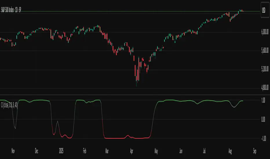
Floating Bands of the Argentine Peso (Sebastian.Waisgold)
The BCRA ( Central Bank of the Argentine Republic ) announced that as of Monday, April 15, 2025, the Argentine Peso (USDARS) will float within a system of divergent exchange rate bands.
The upper band was set at ARS 1400 per USD on 15/04/2025, with a +1% monthly adjustment distributed daily, rising by a fraction each day.
The lower band was set at ARS 1000 per USD on 15/04/2025, with a –1% monthly adjustment distributed daily, falling by a fraction each day.
This indicator is crucial for anyone trading USDARS, since the BCRA will only intervene in these situations:
- Selling : if the Peso depreciates against the USD above the upper band .
- Buying : if the Peso appreciates against the USD below the lower band .
Therefore, this indicator can be used as follows:
- If USDARS is above the upper band , it is “expensive” and you may sell .
- If USDARS is below the lower band , it is “cheap” and you may buy .
It can also be applied to other assets such as:
- USDTARS
- Dollar Cable / CCL (Contado con Liquidación) , derived from the BCBA:YPFD / NYSE:YPF ratio.
A mid band —exactly halfway between the upper and lower bands—has also been added.
Once added, the indicator should look like this:
In the following image you can see:
- Upper Floating Band
- Lower Floating Band
- Mid Floating Band
User Configuration
By double-clicking any line you can adjust:
- Start day (Dia de incio), month (Mes de inicio), and year (Año de inicio)
- Initial upper band value (Valor inicial banda superior)
- Initial lower band value (Valor inicial banda inferior)
- Monthly rate Tasa mensual %)
It is recommended not to modify these settings for the Argentine Peso, as they reflect the BCRA’s official framework. However, you may customize them—and the line colors—for other assets or currencies implementing a similar band scheme.
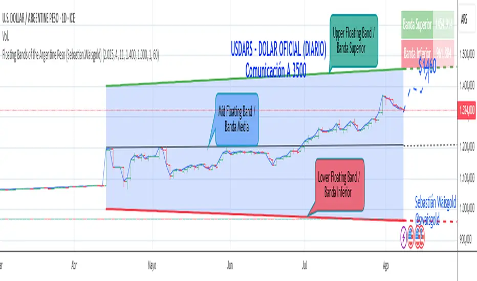
MSTY-WNTR Rebalancing SignalMSTY-WNTR Rebalancing Signal
## Overview
The **MSTY-WNTR Rebalancing Signal** is a custom TradingView indicator designed to help investors dynamically allocate between two YieldMax ETFs: **MSTY** (YieldMax MSTR Option Income Strategy ETF) and **WNTR** (YieldMax Short MSTR Option Income Strategy ETF). These ETFs are tied to MicroStrategy (MSTR) stock, which is heavily influenced by Bitcoin's price due to MSTR's significant Bitcoin holdings.
MSTY benefits from upward movements in MSTR (and thus Bitcoin) through a covered call strategy that generates income but caps upside potential. WNTR, on the other hand, provides inverse exposure, profiting from MSTR declines but losing in rallies. This indicator uses Bitcoin's momentum and MSTR's relative strength to signal when to hold MSTY (bullish phases), WNTR (bearish phases), or stay neutral, aiming to optimize returns by switching allocations at key turning points.
Inspired by strategies discussed in crypto communities (e.g., X posts analyzing MSTR-linked ETFs), this indicator promotes an active rebalancing approach over a "set and forget" buy-and-hold strategy. In simulated backtests over the past 12 months (as of August 4, 2025), the optimized version has shown potential to outperform holding 100% MSTY or 100% WNTR alone, with an illustrative APY of ~125% vs. ~6% for MSTY and ~-15% for WNTR in one scenario.
**Important Disclaimer**: This is not financial advice. Past performance does not guarantee future results. Always consult a financial advisor. Trading involves risk, and you could lose money. The indicator is for educational and informational purposes only.
## Key Features
- **Momentum-Based Signals**: Uses a Simple Moving Average (SMA) on Bitcoin's price to detect bullish (price > SMA) or bearish (price < SMA) trends.
- **RSI Confirmation**: Incorporates MSTR's Relative Strength Index (RSI) to filter signals, avoiding overbought conditions for MSTY and oversold for WNTR.
- **Visual Cues**:
- Green upward triangle for "Hold MSTY".
- Red downward triangle for "Hold WNTR".
- Yellow cross for "Switch" signals.
- Background color: Green for MSTY, red for WNTR.
- **Information Panel**: A table in the top-right corner displays real-time data: BTC Price, SMA value, MSTR RSI, and current Allocation (MSTY, WNTR, or Neutral).
- **Alerts**: Configurable alerts for holding MSTY, holding WNTR, or switching.
- **Optimized Parameters**: Defaults are tuned (SMA: 10 days, RSI: 15 periods, Overbought: 80, Oversold: 20) based on simulations to reduce whipsaws and capture trends effectively.
## How It Works
The indicator's logic is straightforward yet effective for volatile assets like Bitcoin and MSTR:
1. **Primary Trigger (Bitcoin Momentum)**:
- Calculate the SMA of Bitcoin's closing price (default: 10-day).
- Bullish: Current BTC price > SMA → Potential MSTY hold.
- Bearish: Current BTC price < SMA → Potential WNTR hold.
2. **Secondary Filter (MSTR RSI Confirmation)**:
- Compute RSI on MSTR stock (default: 15-period).
- For bullish signals: If RSI > Overbought (80), signal Neutral (avoid overextended rallies).
- For bearish signals: If RSI < Oversold (20), signal Neutral (avoid capitulation bottoms).
3. **Allocation Rules**:
- Hold 100% MSTY if bullish and not overbought.
- Hold 100% WNTR if bearish and not oversold.
- Neutral otherwise (e.g., during choppy or extreme markets) – consider holding cash or avoiding trades.
4. **Rebalancing**:
- Switch signals trigger when the hold changes (e.g., from MSTY to WNTR).
- Recommended frequency: Weekly reviews or on 5% BTC moves to minimize trading costs (aim for 4-6 trades/year).
This approach leverages Bitcoin's influence on MSTR while mitigating the risks of MSTY's covered call drag during downtrends and WNTR's losses in uptrends.
## Setup and Usage
1. **Chart Requirements**:
- Apply this indicator to a Bitcoin chart (e.g., BTCUSD on Binance or Coinbase, daily timeframe recommended).
- Ensure MSTR stock data is accessible (TradingView supports it natively).
2. **Adding to TradingView**:
- Open the Pine Editor.
- Paste the script code.
- Save and add to your chart.
- Customize inputs if needed (e.g., adjust SMA/RSI lengths for different timeframes).
3. **Interpretation**:
- **Green Background/Triangle**: Allocate 100% to MSTY – Bitcoin is in an uptrend, MSTR not overbought.
- **Red Background/Triangle**: Allocate 100% to WNTR – Bitcoin in downtrend, MSTR not oversold.
- **Yellow Switch Cross**: Rebalance your portfolio immediately.
- **Neutral (No Signal)**: Panel shows "Neutral" – Hold cash or previous position; reassess weekly.
- Monitor the panel for key metrics to validate signals manually.
4. **Backtesting and Strategy Integration**:
- Convert to a strategy script by changing `indicator()` to `strategy()` and adding entry/exit logic for automated testing.
- In simulations (e.g., using Python or TradingView's backtester), it has outperformed buy-and-hold in volatile markets by ~100-200% relative APY, but results vary.
- Factor in fees: ETF expense ratios (~0.99%), trading commissions (~$0.40/trade), and slippage.
5. **Risk Management**:
- Use with a diversified portfolio; never allocate more than you can afford to lose.
- Add stop-losses (e.g., 10% trailing) to protect against extreme moves.
- Rebalance sparingly to avoid over-trading in sideways markets.
- Dividends: Reinvest MSTY/WNTR payouts into the current hold for compounding.
## Performance Insights (Simulated as of August 4, 2025)
Based on synthetic backtests modeling the last 12 months:
- **Optimized Strategy APY**: ~125% (by timing switches effectively).
- **Hold 100% MSTY APY**: ~6% (gains from BTC rallies offset by downtrends).
- **Hold 100% WNTR APY**: ~-15% (losses in bull phases outweigh bear gains).
In one scenario with stronger volatility, the strategy achieved ~4533% APY vs. 10% for MSTY and -34% for WNTR, highlighting its potential in dynamic markets. However, these are illustrative; real results depend on actual BTC/MSTR movements. Test thoroughly on historical data.
## Limitations and Considerations
- **Data Dependency**: Relies on accurate BTC and MSTR data; delays or gaps can affect signals.
- **Market Risks**: Bitcoin's volatility can lead to false signals (whipsaws); the RSI filter helps but isn't perfect.
- **No Guarantees**: This indicator doesn't predict the future. MSTR's correlation to BTC may change (e.g., due to regulatory events).
- **Not for All Users**: Best for intermediate/advanced traders familiar with ETFs and crypto. Beginners should paper trade first.
- **Updates**: As of August 4, 2025, this is version 1.0. Future updates may include volume filters or EMA options.
If you find this indicator useful, consider leaving a like or comment on TradingView. Feedback welcome for improvements!

z-score-calkusi-v1.143z-scores incorporate the moment of N look-back bars to allow future price projection.
z-score = (X - mean)/std.deviation ; X = close
z-scores update with each new close print and with each new bar. Each new bar augments the mean and std.deviation for the N bars considered. The old Nth bar falls away from consideration with each new historical bar.
The indicator allows two other options for X: RSI or Moving Average.
NOTE: While trading use the "price" option only.
The other two options are provided for visualisation of RSI and Moving Average as z-score curves.
Use z-scores to identify tops and bottoms in the future as well as intermediate intersections through which a z-score will pass through with each new close and each new bar.
Draw lines from peaks and troughs in the past through intermediate peaks and troughs to identify projected intersections in the future. The most likely intersections are those that are formed from a line that comes from a peak in the past and another line that comes from a trough in the past. Try getting at least two lines from historical peaks and two lines from historical troughs to pass through a future intersection.
Compute the target intersection price in the future by clicking on the z-score indicator header to see a drag-able horizontal line to drag over the intersection. The target price is the last value displayed in the indicator's status bar after the closing price.
When the indicator header is clicked, a white horizontal drag-able line will appear to allow dragging the line over an intersection that has been drawn on the indicator for a future z-score projection and the associated future closing price.
With each new bar that appears, it is necessary to repeat the procedure of clicking the z-score indicator header to be able to drag the drag-able horizontal line to see the new target price for the selected intersection. The projected price will be different from the current close price providing a price arbitrage in time.
New intermediate peaks and troughs that appear require new lines be drawn from the past through the new intermediate peak to find a new intersection in the future and a new projected price. Since z-score curves are sort of cyclical in nature, it is possible to see where one has to locate a future intersection by drawing lines from past peaks and troughs.
Do not get fixated on any one projected price as the market decides which projected price will be realised. All prospective targets should be manually updated with each new bar.
When the z-score plot moves outside a channel comprised of lines that are drawn from the past, be ready to adjust to new market conditions.
z-score plots that move above the zero line indicate price action that is either rising or ranging. Similarly, z-score plots that move below the zero line indicate price action that is either falling or ranging. Be ready to adjust to new market conditions when z-scores move back and forth across the zero line.
A bar with highest absolute z-score for a cycle screams "reversal approaching" and is followed by a bar with a lower absolute z-score where close price tops and bottoms are realised. This can occur either on the next bar or a few bars later.
The indicator also displays the required N for a Normal(0,1) distribution that can be set for finer granularity for the z-score curve.This works with the Confidence Interval (CI) z-score setting. The default z-score is 1.96 for 95% CI.
Common Confidence Interval z-scores to find N for Normal(0,1) with a Margin of Error (MOE) of 1:
70% 1.036
75% 1.150
80% 1.282
85% 1.440
90% 1.645
95% 1.960
98% 2.326
99% 2.576
99.5% 2.807
99.9% 3.291
99.99% 3.891
99.999% 4.417
9-Jun-2025
Added a feature to display price projection labels at z-score levels 3, 2, 1, 0, -1, -2, 3.
This provides a range for prices available at the current time to help decide whether it is worth entering a trade. If the range of prices from say z=|2| to z=|1| is too narrow, then a trade at the current time may not be worth the risk.
Added plot for z-score moving average.
28-Jun-2025
Added Settings option for # of Std.Deviation level Price Labels to display. The default is 3. Min is 2. Max is 6.
This feature allows likelihood assessment for Fibonacci price projections from higher time frames at lower time frames. A Fibonacci price projection that falls outside |3.x| Std.Deviations is not likely.
Added Settings option for Chart Bar Count and Target Label Offset to allow placement of price labels for the standard z-score levels to the right of the window so that these are still visible in the window.
Target Label Offset allows adjustment of placement of Target Price Label in cases when the Target Price Label is either obscured by the price labels for the standard z-score levels or is too far right to be visible in the window.
9-Jul-2025
z-score 1.142 updates:
Displays in the status line before the close price the range for the selected Std. Deviation levels specified in Settings and |z-zMa|.
When |z-zMa| > |avg(z-zMa)| and zMa rising, |z-zMa| and zMa displays in aqua.
When |z-zMa| > |avg(z-zMa)| and zMa falling, |z-zMa| and zMa displays in red.
When |z-zMa| <= |avg(z-zMa)|, z and zMa display in gray.
z usually crosses over zMa when zMa is gray but not always. So if cross-over occurs when zMa is not gray, it implies a strong move in progress.
Practice makes perfect.
Use this indicator at your own risk
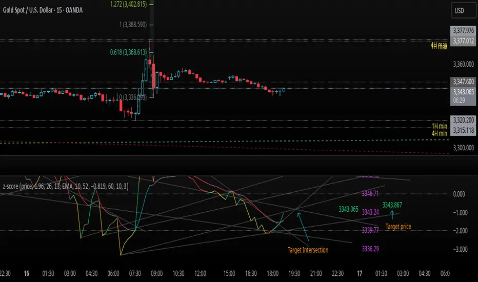
Tuga SupertrendDescription
This strategy uses the Supertrend indicator enhanced with commission and slippage filters to capture trends on the daily chart. It’s designed to work on any asset but is especially effective in markets with consistent movements.
Use the date inputs to set the backtest period (default: from January 1, 2018, through today, June 30, 2025).
The default input values are optimized for the daily chart. For other timeframes, adjust the parameters to suit the asset you’re testing.
Release Notes
June 30, 2025
• Updated default backtest period to end on June 30, 2025.
• Default commission adjusted to 0.1 %.
• Slippage set to 3 ticks.
• Default slippage set to 3 ticks.
• Simplified the strategy name to “Tuga Supertrend”.
Default Parameters
Parameter Default Value
Supertrend Period 10
Multiplier (Factor) 3
Commission 0.1 %
Slippage 3 ticks
Start Date January 1, 2018
End Date June 30, 2025
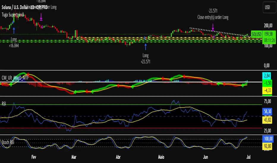
SPX Weekly Expected Moves# SPX Weekly Expected Moves Indicator
A professional Pine Script indicator for TradingView that displays weekly expected move levels for SPX based on real options data, with integrated Fibonacci retracement analysis and intelligent alerting system.
## Overview
This indicator helps options and equity traders visualize weekly expected move ranges for the S&P 500 Index (SPX) by plotting historical and current week expected move boundaries derived from weekly options pricing. Unlike theoretical volatility calculations, this indicator uses actual market-based expected move data that you provide from options platforms.
## Key Features
### 📈 **Expected Move Visualization**
- **Historical Lines**: Display past weeks' expected moves with configurable history (10, 26, or 52 weeks)
- **Current Week Focus**: Highlighted current week with extended lines to present time
- **Friday Close Reference**: Orange baseline showing the previous Friday's close price
- **Timeframe Independent**: Works consistently across all chart timeframes (1m to 1D)
### 🎯 **Fibonacci Integration**
- **Five Fibonacci Levels**: 23.6%, 38.2%, 50%, 61.8%, 76.4% between Friday close and expected move boundaries
- **Color-Coded Levels**:
- Red: 23.6% & 76.4% (outer levels)
- Blue: 38.2% & 61.8% (golden ratio levels)
- Black: 50% (midpoint - most critical level)
- **Current Week Only**: Fibonacci levels shown only for active trading week to reduce clutter
### 📊 **Real-Time Information Table**
- **Current SPX Price**: Live market price
- **Expected Move**: ±EM value for current week
- **Previous Close**: Friday close price (baseline for calculations)
- **100% EM Levels**: Exact upper and lower boundary prices
- **Current Location**: Real-time position within the EM structure (e.g., "Above 38.2% Fib (upper zone)")
### 🚨 **Intelligent Alert System**
- **Zone-Aware Alerts**: Separate alerts for upper and lower zones
- **Key Level Breaches**: Alerts for 23.6% and 76.4% Fibonacci level crossings
- **Bar Close Based**: Alerts trigger on confirmed bar closes, not tick-by-tick
- **Customizable**: Enable/disable alerts through settings
## How It Works
### Data Input Method
The indicator uses a **manual data entry approach** where you input actual expected move values obtained from options platforms:
```pinescript
// Add entries using the options expiration Friday date
map.put(expected_moves, 20250613, 91.244) // Week ending June 13, 2025
map.put(expected_moves, 20250620, 95.150) // Week ending June 20, 2025
```
### Weekly Structure
- **Monday 9:30 AM ET**: Week begins
- **Friday 4:00 PM ET**: Week ends
- **Lines Extend**: From Monday open to Friday close (historical) or current time + 5 bars (current week)
- **Timezone Handling**: Uses "America/New_York" for proper DST handling
### Calculation Logic
1. **Base Price**: Previous Friday's SPX close price
2. **Expected Move**: Market-derived ±EM value from weekly options
3. **Upper Boundary**: Friday Close + Expected Move
4. **Lower Boundary**: Friday Close - Expected Move
5. **Fibonacci Levels**: Proportional levels between Friday close and EM boundaries
## Setup Instructions
### 1. Data Collection
Obtain weekly expected move values from options platforms such as:
- **ThinkOrSwim**: Use thinkBack feature to look up weekly expected moves
- **Tastyworks**: Check weekly options expected move data
- **CBOE**: Reference SPX weekly options data
- **Manual Calculation**: (ATM Call Premium + ATM Put Premium) × 0.85
### 2. Data Entry
After each Friday close, update the indicator with the next week's expected move:
```pinescript
// Example: On Friday June 7, 2025, add data for week ending June 13
map.put(expected_moves, 20250613, 91.244) // Actual EM value from your platform
```
### 3. Configuration
Customize the indicator through the settings panel:
#### Visual Settings
- **Show Current Week EM**: Toggle current week display
- **Show Past Weeks**: Toggle historical weeks display
- **Max Weeks History**: Choose 10, 26, or 52 weeks of history
- **Show Fibonacci Levels**: Toggle Fibonacci retracement levels
- **Label Controls**: Customize which labels to display
#### Colors
- **Current Week EM**: Default yellow for active week
- **Past Weeks EM**: Default gray for historical weeks
- **Friday Close**: Default orange for baseline
- **Fibonacci Levels**: Customizable colors for each level type
#### Alerts
- **Enable EM Breach Alerts**: Master toggle for all alerts
- **Specific Alerts**: Four alert types for Fibonacci level breaches
## Trading Applications
### Options Trading
- **Straddle/Strangle Positioning**: Visualize breakeven levels for neutral strategies
- **Directional Plays**: Assess probability of reaching target levels
- **Earnings Plays**: Compare actual vs. expected move outcomes
### Equity Trading
- **Support/Resistance**: Use EM boundaries and Fibonacci levels as key levels
- **Breakout Trading**: Monitor for moves beyond expected ranges
- **Mean Reversion**: Look for reversals at extreme Fibonacci levels
### Risk Management
- **Position Sizing**: Gauge likely price ranges for the week
- **Stop Placement**: Use Fibonacci levels for logical stop locations
- **Profit Targets**: Set targets based on EM structure probabilities
## Technical Implementation
### Performance Features
- **Memory Managed**: Configurable history limits prevent memory issues
- **Timeframe Independent**: Uses timestamp-based calculations for consistency
- **Object Management**: Automatic cleanup of drawing objects prevents duplicates
- **Error Handling**: Robust bounds checking and NA value handling
### Pine Script Best Practices
- **v6 Compliance**: Uses latest Pine Script version features
- **User Defined Types**: Structured data management with WeeklyEM type
- **Efficient Drawing**: Smart line/label creation and deletion
- **Professional Standards**: Clean code organization and comprehensive documentation
## Customization Guide
### Adding New Weeks
```pinescript
// Add after market close each Friday
map.put(expected_moves, YYYYMMDD, EM_VALUE)
```
### Color Schemes
Customize colors for different trading styles:
- **Dark Theme**: Use bright colors for visibility
- **Light Theme**: Use contrasting dark colors
- **Minimalist**: Use single color with transparency
### Label Management
Control label density:
- **Show Current Week Labels Only**: Reduce clutter for active trading
- **Show All Labels**: Full information for analysis
- **Selective Display**: Choose specific label types
## Troubleshooting
### Common Issues
1. **No Lines Appearing**: Check that expected move data is entered for current/recent weeks
2. **Wrong Time Display**: Ensure "America/New_York" timezone is properly handled
3. **Duplicate Lines**: Restart indicator if drawing objects appear duplicated
4. **Missing Fibonacci Levels**: Verify "Show Fibonacci Levels" is enabled
### Data Validation
- **Expected Move Format**: Use positive numbers (e.g., 91.244, not ±91.244)
- **Date Format**: Use YYYYMMDD format (e.g., 20250613)
- **Reasonable Values**: Verify EM values are realistic (typically 50-200 for SPX)
## Version History
### Current Version
- **Pine Script v6**: Latest version compatibility
- **Fibonacci Integration**: Five-level retracement analysis
- **Zone-Aware Alerts**: Upper/lower zone differentiation
- **Dynamic Line Management**: Smart current week extension
- **Professional UI**: Comprehensive information table
### Future Enhancements
- **Multiple Symbols**: Extend beyond SPX to other indices
- **Automated Data**: Integration with options data APIs
- **Statistical Analysis**: Success rate tracking for EM predictions
- **Additional Levels**: Custom percentage levels beyond Fibonacci
## License & Usage
This indicator is designed for educational and trading purposes. Users are responsible for:
- **Data Accuracy**: Ensuring correct expected move values
- **Risk Management**: Proper position sizing and risk controls
- **Market Understanding**: Comprehending options-based expected move concepts
## Support
For questions, issues, or feature requests related to this indicator, please refer to the code comments and documentation within the Pine Script file.
---
**Disclaimer**: This indicator is for informational purposes only. Trading involves substantial risk of loss and is not suitable for all investors. Past performance does not guarantee future results.
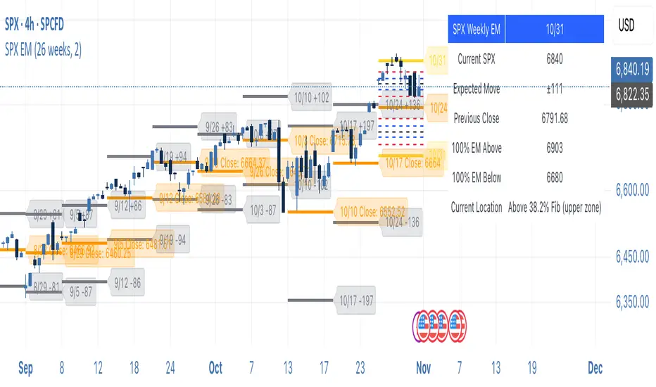
Liquid Pulse Liquid Pulse by Dskyz (DAFE) Trading Systems
Liquid Pulse is a trading algo built by Dskyz (DAFE) Trading Systems for futures markets like NQ1!, designed to snag high-probability trades with tight risk control. it fuses a confluence system—VWAP, MACD, ADX, volume, and liquidity sweeps—with a trade scoring setup, daily limits, and VIX pauses to dodge wild volatility. visuals include simple signals, VWAP bands, and a dashboard with stats.
Core Components for Liquid Pulse
Volume Sensitivity (volumeSensitivity) controls how much volume spikes matter for entries. options: 'Low', 'Medium', 'High' default: 'High' (catches small spikes, good for active markets) tweak it: 'Low' for calm markets, 'High' for chaos.
MACD Speed (macdSpeed) sets the MACD’s pace for momentum. options: 'Fast', 'Medium', 'Slow' default: 'Medium' (solid balance) tweak it: 'Fast' for scalping, 'Slow' for swings.
Daily Trade Limit (dailyTradeLimit) caps trades per day to keep risk in check. range: 1 to 30 default: 20 tweak it: 5-10 for safety, 20-30 for action.
Number of Contracts (numContracts) sets position size. range: 1 to 20 default: 4 tweak it: up for big accounts, down for small.
VIX Pause Level (vixPauseLevel) stops trading if VIX gets too hot. range: 10 to 80 default: 39.0 tweak it: 30 to avoid volatility, 50 to ride it.
Min Confluence Conditions (minConditions) sets how many signals must align. range: 1 to 5 default: 2 tweak it: 3-4 for strict, 1-2 for more trades.
Min Trade Score (Longs/Shorts) (minTradeScoreLongs/minTradeScoreShorts) filters trade quality. longs range: 0 to 100 default: 73 shorts range: 0 to 100 default: 75 tweak it: 80-90 for quality, 60-70 for volume.
Liquidity Sweep Strength (sweepStrength) gauges breakouts. range: 0.1 to 1.0 default: 0.5 tweak it: 0.7-1.0 for strong moves, 0.3-0.5 for small.
ADX Trend Threshold (adxTrendThreshold) confirms trends. range: 10 to 100 default: 41 tweak it: 40-50 for trends, 30-35 for weak ones.
ADX Chop Threshold (adxChopThreshold) avoids chop. range: 5 to 50 default: 20 tweak it: 15-20 to dodge chop, 25-30 to loosen.
VWAP Timeframe (vwapTimeframe) sets VWAP period. options: '15', '30', '60', '240', 'D' default: '60' (1-hour) tweak it: 60 for day, 240 for swing, D for long.
Take Profit Ticks (Longs/Shorts) (takeProfitTicksLongs/takeProfitTicksShorts) sets profit targets. longs range: 5 to 100 default: 25.0 shorts range: 5 to 100 default: 20.0 tweak it: 30-50 for trends, 10-20 for chop.
Max Profit Ticks (maxProfitTicks) caps max gain. range: 10 to 200 default: 60.0 tweak it: 80-100 for big moves, 40-60 for tight.
Min Profit Ticks to Trail (minProfitTicksTrail) triggers trailing. range: 1 to 50 default: 7.0 tweak it: 10-15 for big gains, 5-7 for quick locks.
Trailing Stop Ticks (trailTicks) sets trail distance. range: 1 to 50 default: 5.0 tweak it: 8-10 for room, 3-5 for fast locks.
Trailing Offset Ticks (trailOffsetTicks) sets trail offset. range: 1 to 20 default: 2.0 tweak it: 1-2 for tight, 5-10 for loose.
ATR Period (atrPeriod) measures volatility. range: 5 to 50 default: 9 tweak it: 14-20 for smooth, 5-9 for reactive.
Hardcoded Settings volLookback: 30 ('Low'), 20 ('Medium'), 11 ('High') volThreshold: 1.5 ('Low'), 1.8 ('Medium'), 2 ('High') swingLen: 5
Execution Logic Overview trades trigger when confluence conditions align, entering long or short with set position sizes. exits use dynamic take-profits, trailing stops after a profit threshold, hard stops via ATR, and a time stop after 100 bars.
Features Multi-Signal Confluence: needs VWAP, MACD, volume, sweeps, and ADX to line up.
Risk Control: ATR-based stops (capped 15 ticks), take-profits (scaled by volatility), and trails.
Market Filters: VIX pause, ADX trend/chop checks, volatility gates. Dashboard: shows scores, VIX, ADX, P/L, win %, streak.
Visuals Simple signals (green up triangles for longs, red down for shorts) and VWAP bands with glow. info table (bottom right) with MACD momentum. dashboard (top right) with stats.
Chart and Backtest:
NQ1! futures, 5-minute chart. works best in trending, volatile conditions. tweak inputs for other markets—test thoroughly.
Backtesting: NQ1! Frame: Jan 19, 2025, 09:00 — May 02, 2025, 16:00 Slippage: 3 Commission: $4.60
Fee Typical Range (per side, per contract)
CME Exchange $1.14 – $1.20
Clearing $0.10 – $0.30
NFA Regulatory $0.02
Firm/Broker Commis. $0.25 – $0.80 (retail prop)
TOTAL $1.60 – $2.30 per side
Round Turn: (enter+exit) = $3.20 – $4.60 per contract
Disclaimer this is for education only. past results don’t predict future wins. trading’s risky—only use money you can lose. backtest and validate before going live. (expect moderators to nitpick some random chart symbol rule—i’ll fix and repost if they pull it.)
About the Author Dskyz (DAFE) Trading Systems crafts killer trading algos. Liquid Pulse is pure research and grit, built for smart, bold trading. Use it with discipline. Use it with clarity. Trade smarter. I’ll keep dropping badass strategies ‘til i build a brand or someone signs me up.
2025 Created by Dskyz, powered by DAFE Trading Systems. Trade smart, trade bold.
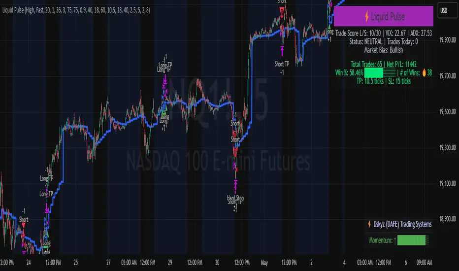
Bitcoin Polynomial Regression ModelThis is the main version of the script. Click here for the Oscillator part of the script.
💡Why this model was created:
One of the key issues with most existing models, including our own Bitcoin Log Growth Curve Model , is that they often fail to realistically account for diminishing returns. As a result, they may present overly optimistic bull cycle targets (hence, we introduced alternative settings in our previous Bitcoin Log Growth Curve Model).
This new model however, has been built from the ground up with a primary focus on incorporating the principle of diminishing returns. It directly responds to this concept, which has been briefly explored here .
📉The theory of diminishing returns:
This theory suggests that as each four-year market cycle unfolds, volatility gradually decreases, leading to more tempered price movements. It also implies that the price increase from one cycle peak to the next will decrease over time as the asset matures. The same pattern applies to cycle lows and the relationship between tops and bottoms. In essence, these price movements are interconnected and should generally follow a consistent pattern. We believe this model provides a more realistic outlook on bull and bear market cycles.
To better understand this theory, the relationships between cycle tops and bottoms are outlined below:https://www.tradingview.com/x/7Hldzsf2/
🔧Creation of the model:
For those interested in how this model was created, the process is explained here. Otherwise, feel free to skip this section.
This model is based on two separate cubic polynomial regression lines. One for the top price trend and another for the bottom. Both follow the general cubic polynomial function:
ax^3 +bx^2 + cx + d.
In this equation, x represents the weekly bar index minus an offset, while a, b, c, and d are determined through polynomial regression analysis. The input (x, y) values used for the polynomial regression analysis are as follows:
Top regression line (x, y) values:
113, 18.6
240, 1004
451, 19128
655, 65502
Bottom regression line (x, y) values:
103, 2.5
267, 211
471, 3193
676, 16255
The values above correspond to historical Bitcoin cycle tops and bottoms, where x is the weekly bar index and y is the weekly closing price of Bitcoin. The best fit is determined using metrics such as R-squared values, residual error analysis, and visual inspection. While the exact details of this evaluation are beyond the scope of this post, the following optimal parameters were found:
Top regression line parameter values:
a: 0.000202798
b: 0.0872922
c: -30.88805
d: 1827.14113
Bottom regression line parameter values:
a: 0.000138314
b: -0.0768236
c: 13.90555
d: -765.8892
📊Polynomial Regression Oscillator:
This publication also includes the oscillator version of the this model which is displayed at the bottom of the screen. The oscillator applies a logarithmic transformation to the price and the regression lines using the formula log10(x) .
The log-transformed price is then normalized using min-max normalization relative to the log-transformed top and bottom regression line with the formula:
normalized price = log(close) - log(bottom regression line) / log(top regression line) - log(bottom regression line)
This transformation results in a price value between 0 and 1 between both the regression lines. The Oscillator version can be found here.
🔍Interpretation of the Model:
In general, the red area represents a caution zone, as historically, the price has often been near its cycle market top within this range. On the other hand, the green area is considered an area of opportunity, as historically, it has corresponded to the market bottom.
The top regression line serves as a signal for the absolute market cycle peak, while the bottom regression line indicates the absolute market cycle bottom.
Additionally, this model provides a predicted range for Bitcoin's future price movements, which can be used to make extrapolated predictions. We will explore this further below.
🔮Future Predictions:
Finally, let's discuss what this model actually predicts for the potential upcoming market cycle top and the corresponding market cycle bottom. In our previous post here , a cycle interval analysis was performed to predict a likely time window for the next cycle top and bottom:
In the image, it is predicted that the next top-to-top cycle interval will be 208 weeks, which translates to November 3rd, 2025. It is also predicted that the bottom-to-top cycle interval will be 152 weeks, which corresponds to October 13th, 2025. On the macro level, these two dates align quite well. For our prediction, we take the average of these two dates: October 24th 2025. This will be our target date for the bull cycle top.
Now, let's do the same for the upcoming cycle bottom. The bottom-to-bottom cycle interval is predicted to be 205 weeks, which translates to October 19th, 2026, and the top-to-bottom cycle interval is predicted to be 259 weeks, which corresponds to October 26th, 2026. We then take the average of these two dates, predicting a bear cycle bottom date target of October 19th, 2026.
Now that we have our predicted top and bottom cycle date targets, we can simply reference these two dates to our model, giving us the Bitcoin top price prediction in the range of 152,000 in Q4 2025 and a subsequent bottom price prediction in the range of 46,500 in Q4 2026.
For those interested in understanding what this specifically means for the predicted diminishing return top and bottom cycle values, the image below displays these predicted values. The new values are highlighted in yellow:
And of course, keep in mind that these targets are just rough estimates. While we've done our best to estimate these targets through a data-driven approach, markets will always remain unpredictable in nature. What are your targets? Feel free to share them in the comment section below.

Bitcoin Polynomial Regression OscillatorThis is the oscillator version of the script. Click here for the other part of the script.
💡Why this model was created:
One of the key issues with most existing models, including our own Bitcoin Log Growth Curve Model , is that they often fail to realistically account for diminishing returns. As a result, they may present overly optimistic bull cycle targets (hence, we introduced alternative settings in our previous Bitcoin Log Growth Curve Model).
This new model however, has been built from the ground up with a primary focus on incorporating the principle of diminishing returns. It directly responds to this concept, which has been briefly explored here .
📉The theory of diminishing returns:
This theory suggests that as each four-year market cycle unfolds, volatility gradually decreases, leading to more tempered price movements. It also implies that the price increase from one cycle peak to the next will decrease over time as the asset matures. The same pattern applies to cycle lows and the relationship between tops and bottoms. In essence, these price movements are interconnected and should generally follow a consistent pattern. We believe this model provides a more realistic outlook on bull and bear market cycles.
To better understand this theory, the relationships between cycle tops and bottoms are outlined below:https://www.tradingview.com/x/7Hldzsf2/
🔧Creation of the model:
For those interested in how this model was created, the process is explained here. Otherwise, feel free to skip this section.
This model is based on two separate cubic polynomial regression lines. One for the top price trend and another for the bottom. Both follow the general cubic polynomial function:
ax^3 +bx^2 + cx + d.
In this equation, x represents the weekly bar index minus an offset, while a, b, c, and d are determined through polynomial regression analysis. The input (x, y) values used for the polynomial regression analysis are as follows:
Top regression line (x, y) values:
113, 18.6
240, 1004
451, 19128
655, 65502
Bottom regression line (x, y) values:
103, 2.5
267, 211
471, 3193
676, 16255
The values above correspond to historical Bitcoin cycle tops and bottoms, where x is the weekly bar index and y is the weekly closing price of Bitcoin. The best fit is determined using metrics such as R-squared values, residual error analysis, and visual inspection. While the exact details of this evaluation are beyond the scope of this post, the following optimal parameters were found:
Top regression line parameter values:
a: 0.000202798
b: 0.0872922
c: -30.88805
d: 1827.14113
Bottom regression line parameter values:
a: 0.000138314
b: -0.0768236
c: 13.90555
d: -765.8892
📊Polynomial Regression Oscillator:
This publication also includes the oscillator version of the this model which is displayed at the bottom of the screen. The oscillator applies a logarithmic transformation to the price and the regression lines using the formula log10(x) .
The log-transformed price is then normalized using min-max normalization relative to the log-transformed top and bottom regression line with the formula:
normalized price = log(close) - log(bottom regression line) / log(top regression line) - log(bottom regression line)
This transformation results in a price value between 0 and 1 between both the regression lines.
🔍Interpretation of the Model:
In general, the red area represents a caution zone, as historically, the price has often been near its cycle market top within this range. On the other hand, the green area is considered an area of opportunity, as historically, it has corresponded to the market bottom.
The top regression line serves as a signal for the absolute market cycle peak, while the bottom regression line indicates the absolute market cycle bottom.
Additionally, this model provides a predicted range for Bitcoin's future price movements, which can be used to make extrapolated predictions. We will explore this further below.
🔮Future Predictions:
Finally, let's discuss what this model actually predicts for the potential upcoming market cycle top and the corresponding market cycle bottom. In our previous post here , a cycle interval analysis was performed to predict a likely time window for the next cycle top and bottom:
In the image, it is predicted that the next top-to-top cycle interval will be 208 weeks, which translates to November 3rd, 2025. It is also predicted that the bottom-to-top cycle interval will be 152 weeks, which corresponds to October 13th, 2025. On the macro level, these two dates align quite well. For our prediction, we take the average of these two dates: October 24th 2025. This will be our target date for the bull cycle top.
Now, let's do the same for the upcoming cycle bottom. The bottom-to-bottom cycle interval is predicted to be 205 weeks, which translates to October 19th, 2026, and the top-to-bottom cycle interval is predicted to be 259 weeks, which corresponds to October 26th, 2026. We then take the average of these two dates, predicting a bear cycle bottom date target of October 19th, 2026.
Now that we have our predicted top and bottom cycle date targets, we can simply reference these two dates to our model, giving us the Bitcoin top price prediction in the range of 152,000 in Q4 2025 and a subsequent bottom price prediction in the range of 46,500 in Q4 2026.
For those interested in understanding what this specifically means for the predicted diminishing return top and bottom cycle values, the image below displays these predicted values. The new values are highlighted in yellow:
And of course, keep in mind that these targets are just rough estimates. While we've done our best to estimate these targets through a data-driven approach, markets will always remain unpredictable in nature. What are your targets? Feel free to share them in the comment section below.
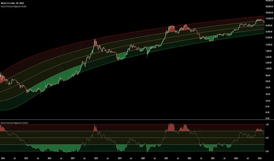
Inyerneck Sniper Engine v4.2 — FINAL WORKING 2025yer momUltra-aggressive momentum sniper built for pennies & BTC.
Fires on every volume explosion + EMA snap. No mercy, no filters.
50+ trades per month. Use small size or die trying.
Private alpha —
