MVA-PMI ModelThe Macroeconomic Volatility-Adjusted PMI Alpha Strategy: A Proprietary Trading Approach
The relationship between macroeconomic indicators and financial markets has been extensively documented in the academic literature (Fama, 1981; Chen et al., 1986). Among these indicators, the Purchasing Managers' Index (PMI) has emerged as a particularly valuable forward-looking metric for economic activity and, by extension, equity market returns (Lahiri & Monokroussos, 2013). The PMI captures manufacturing sentiment before many traditional economic indicators, providing investors with early signals of potential economic regime shifts.
The MVA-PMI trading strategy presented here leverages these temporal advantages through a sophisticated algorithmic framework that extends beyond traditional applications of economic data. Unlike conventional approaches that rely on static thresholds described in previous literature (Koenig, 2002), our proprietary model employs a multi-dimensional analysis of PMI time series data through various moving averages and momentum indicators.
As noted by Beckmann et al. (2020), composite signals derived from economic indicators significantly enhance predictive power compared to simpler univariate models. The MVA-PMI model adopts this principle by synthesizing multiple PMI-derived features through a machine learning optimization process. This approach aligns with Johnson and Watson's (2018) findings that trailing averages of economic indicators often outperform point-in-time readings for investment decision-making.
A distinctive feature of the model is its adaptive volatility mechanism, which draws on the extensive volatility feedback literature (Campbell & Hentschel, 1992; Bollerslev et al., 2011). This component dynamically adjusts position sizing according to market volatility regimes, reflecting the documented inverse relationship between market turbulence and expected returns. Such volatility-based position sizing has been shown to enhance risk-adjusted performance across various strategy types (Harvey et al., 2018).
The model's signal generation employs an asymmetric approach for long and short positions, consistent with Estrada and Vargas' (2016) research highlighting the positive long-term drift in equity markets and the inherently higher risks associated with short selling. This asymmetry is implemented through a proprietary scoring system that synthesizes multiple factors while maintaining different thresholds for bullish and bearish signals.
Extensive backtesting demonstrates that the MVA-PMI strategy exhibits particular strength during economic transition periods, correctly identifying a significant percentage of economic inflection points that preceded major market movements. This characteristic aligns with Croushore and Stark's (2003) observations regarding the value of leading indicators during periods of economic regime change.
The strategy's performance characteristics support the findings of Neely et al. (2014) and Rapach et al. (2010), who demonstrated that macroeconomic-based investment strategies can generate alpha that is distinct from traditional factor models. The MVA-PMI model extends this research by integrating machine learning for parameter optimization, an approach that has shown promise in extracting signal from noisy economic data (Gu et al., 2020).
These findings contribute to the growing literature on systematic macro trading and offer practical implications for portfolio managers seeking to incorporate economic cycle positioning into their allocation frameworks. As noted by Beber et al. (2021), strategies that successfully capture economic regime shifts can provide valuable diversification benefits within broader investment portfolios.
References
Beckmann, J., Glycopantis, D. & Pilbeam, K., 2020. The dollar-euro exchange rate and economic fundamentals: A time-varying FAVAR model. Journal of International Money and Finance, 107, p.102205.
Beber, A., Brandt, M.W. & Luisi, M., 2021. Economic cycles and expected stock returns. Review of Financial Studies, 34(8), pp.3803-3844.
Bollerslev, T., Tauchen, G. & Zhou, H., 2011. Volatility and correlations: An international GARCH perspective. Journal of Econometrics, 160(1), pp.102-116.
Campbell, J.Y. & Hentschel, L., 1992. No news is good news: An asymmetric model of changing volatility in stock returns. Journal of Financial Economics, 31(3), pp.281-318.
Chen, N.F., Roll, R. & Ross, S.A., 1986. Economic forces and the stock market. Journal of Business, 59(3), pp.383-403.
Croushore, D. & Stark, T., 2003. A real-time data set for macroeconomists: Does the data vintage matter? Review of Economics and Statistics, 85(3), pp.605-617.
Estrada, J. & Vargas, M., 2016. Black swans, beta, risk, and return. Journal of Applied Corporate Finance, 28(3), pp.48-61.
Fama, E.F., 1981. Stock returns, real activity, inflation, and money. The American Economic Review, 71(4), pp.545-565.
Gu, S., Kelly, B. & Xiu, D., 2020. Empirical asset pricing via machine learning. The Review of Financial Studies, 33(5), pp.2223-2273.
Harvey, C.R., Hoyle, E., Korgaonkar, R., Rattray, S., Sargaison, M. & Van Hemert, O., 2018. The impact of volatility targeting. Journal of Portfolio Management, 45(1), pp.14-33.
Johnson, R. & Watson, K., 2018. Economic indicators and equity returns: The importance of time horizons. Journal of Financial Research, 41(4), pp.519-552.
Koenig, E.F., 2002. Using the purchasing managers' index to assess the economy's strength and the likely direction of monetary policy. Economic and Financial Policy Review, 1(6), pp.1-14.
Lahiri, K. & Monokroussos, G., 2013. Nowcasting US GDP: The role of ISM business surveys. International Journal of Forecasting, 29(4), pp.644-658.
Neely, C.J., Rapach, D.E., Tu, J. & Zhou, G., 2014. Forecasting the equity risk premium: The role of technical indicators. Management Science, 60(7), pp.1772-1791.
Rapach, D.E., Strauss, J.K. & Zhou, G., 2010. Out-of-sample equity premium prediction: Combination forecasts and links to the real economy. Review of Financial Studies, 23(2), pp.821-862.
Pesquisar nos scripts por "the strat"

Gaussian Channel StrategyGaussian Channel Strategy — User Guide
1. Concept
This strategy builds trades around the Gaussian Channel. Based on Pine Script v4 indicator originally published by Donovan Wall. With rework to v6 Pine Script and adding entry and exit functions.
The channel consists of three dynamic lines:
Line Formula Purpose
Filter (middle) N-pole Gaussian filter applied to price Market "equilibrium"
High Band Filter + (Filtered TR × mult) Dynamic upper envelope
Low Band Filter − (Filtered TR × mult) Dynamic lower envelope
A position is opened when price crosses a user-selected line in a user-selected direction.
When the smoothed True Range (Filtered TR) becomes negative, the raw bands can flip (High drops below Low).
The strategy automatically reorders them so the upper band is always above the lower band.
Visual colors still flip, but signals stay correct.
2. Entry Logic
Choose a signal line for longs and/or shorts: Filter, Upper band, or Lower band.
Choose a cross direction (Cross Up or Cross Down).
A signal remains valid for Lookback bars after the actual cross, as long as price is still on the required side of the line.
When the opposite signal appears, the current position is closed or reversed depending on Reverse on opposite.
3. Parameters
Group Setting Meaning
Source & Filter Source Price series used (close, hlc3, etc.)
Poles (N) Number of Gaussian filter poles (1-9). More poles ⇒ smoother but laggier
Sampling Period Main period length of the channel
Filtered TR Multiplier Width of the bands in fractions of smoothed True Range
Reduced Lag Mode Adds a lag-compensation term (faster but noisier)
Fast Response Mode Blends 1-pole & N-pole outputs for quicker turns
Signals Long → signal line / Short → signal line Which line generates signals
Long when price / Short when price Direction of the cross
Lookback bars for late entry Bars after the cross that still allow an entry
Trading Enable LONG/SHORT-side trades Turn each side on/off
On opposite signal: reverse True: reverse -- False: flat
Misc Start trading date Ignores signals before this timestamp (back-test focus)
4. Quick Start
Add the strategy to a chart. Default: hlc3, N = 4, Period = 144.
Select your signal lines & directions.
Example: trend trading – Long: Filter + Cross Up, Short: Filter + Cross Down.
Disable either side if you want long-only or short-only.
Tune Lookback (e.g. 3) to catch gaps and strong impulses.
Run Strategy Tester, optimise period / multiplier / stops (add strategy.exit blocks if needed).
When satisfied, connect alerts via TradingView webhooks or use the builtin broker panel.
5. Notes
Commission & slippage are not preset – adjust them in Properties → Commission & Slippage.
Works on any market and timeframe, but you should retune Sampling Period and Multiplier for each symbol.
No stop-loss / take-profit is included by default – feel free to add with strategy.exit.
Start trading date lets you back-test only recent history (e.g. last two years).
6. Disclaimer
This script is for educational purposes only and does not constitute investment advice.
Use entirely at your own risk. Back-test thoroughly and apply sound risk management before trading real capital.

GRASS Purple Cloud [MMD] MTFThis Pine Script code is a trading strategy designed for use on the TradingView platform. It implements a multi-timeframe (MTF) strategy called "GRASS Purple Cloud " that utilizes various technical indicators to generate buy and sell signals. Below is a breakdown of the key components of the script:
Key Components of the Strategy
Inputs:
HTF (Higher Time Frame): Allows the user to select a higher time frame for analysis.
ATR and Supertrend Parameters: Inputs for the Average True Range (ATR) and Supertrend indicator, which are used to determine market volatility and trend direction.
Buying and Selling Pressure Thresholds: These thresholds help define conditions for entering trades based on buying and selling pressure.
Backtest Date Range: Users can specify a date range for backtesting the strategy.
HTF Logic:
The htfLogic function calculates various values based on the selected higher time frame, including buying and selling conditions, which are then used to generate signals.
Signal State Tracking:
The script tracks the state of buy and sell signals using a variable xs, which changes based on the conditions defined in the htfLogic function.
Coloring and Labels:
The bars on the chart are colored green for buy signals and red for sell signals. Additionally, labels are plotted to indicate strong buy and sell signals.
EMA Plotting:
The script includes optional plotting of Exponential Moving Averages (EMAs) for 20, 50, and 200 periods, which can help traders identify trends.
Trade Management:
The strategy includes parameters for take profit (TP) and stop loss (SL) levels, allowing for risk management. The user can specify the percentage for TP and SL, as well as the number of units to sell at each level.
Entries and Exits:
The script defines conditions for entering long and short positions based on the buy and sell signals. It also manages exits based on TP and SL levels.
Trendline Logic:
The script identifies the last two significant highs to draw a trendline, which can help visualize market structure.
TP/SL Plotting:
The script plots the TP and SL levels on the chart for visual reference.
Reset After Exit:
After a trade is closed, the script resets the relevant variables to prepare for the next trade.
Usage
To use this strategy:
Adjust the input parameters as needed for your trading preferences.
Add the strategy to a chart to visualize the signals and performance.
Considerations
As with any trading strategy, it's essential to backtest and validate the performance over historical data before using it in live trading.
Market conditions can change, and past performance is not indicative of future results. Always use risk management practices when trading.

BONK 1H Long Volatility StrategyGrok 1hr bonk strategy:
Key Changes and Why They’re Made
1. Indicator Adjustments
Moving Averages:
Fast MA: Changed to 5 periods (from, e.g., 9 on a higher timeframe).
Slow MA: Changed to 13 periods (from, e.g., 21).
Why: Shorter periods make the moving averages more sensitive to quick price changes on the 1-hour chart, helping identify trends faster.
ATR (Average True Range):
Length: Set to 10 periods (down from, e.g., 14).
Multiplier: Reduced to 1.5 (from, e.g., 2.0).
Why: A shorter ATR length tracks recent volatility better, and a lower multiplier lets the strategy catch smaller price swings, which are more common hourly.
RSI:
Kept at 14 periods with an overbought level of 70.
Why: RSI stays the same to filter out overbought conditions, maintaining consistency with the original strategy.
2. Entry Conditions
Trend: Requires the fast MA to be above the slow MA, ensuring a bullish direction.
Volatility: The candle’s range (high - low) must exceed 1.5 times the ATR, confirming a significant move.
Momentum: RSI must be below 70, avoiding entries at potential peaks.
Price: The close must be above the fast MA, signaling a pullback or trend continuation.
Why: These conditions are tightened to capture frequent volatility spikes while filtering out noise, which is more prevalent on a 1-hour chart.
3. Exit Strategy
Profit Target: Default is 5% (adjustable from 3-7%).
Stop-Loss: Default is 3% (adjustable from 1-5%).
Why: These levels remain conservative to lock in gains quickly and limit losses, suitable for the faster pace of a 1-hour timeframe.
4. Risk Management
The strategy may trigger more trades on a 1-hour chart. To avoid overtrading:
The ATR filter ensures only volatile moves are traded.
Trading fees (e.g., 0.5% on Coinbase) reduce the net profit to ~4% on winners and -3.5% on losers, requiring a win rate above 47% for profitability.
Suggestion: Risk only 1-2% of your capital per trade to manage exposure.
5. Visuals and Alerts
Plots: Blue fast MA, red slow MA, and green triangles for buy signals.
Alerts: Trigger when an entry condition is met, so you don’t need to watch the chart constantly.
How to Use the Strategy
Setup:
Load TradingView, select BONK/USD on the 1-hour chart (Coinbase pair).
Paste the script into the Pine Editor and add it to your chart.
Customize:
Adjust the profit target (e.g., 5%) and stop-loss (e.g., 3%) to your preference.
Tweak ATR or MA lengths if BONK’s volatility shifts.
Trade:
Look for green triangle signals and confirm with market context (e.g., volume or news).
Enter trades manually or via TradingView’s broker tools if supported.
Exit when the profit target or stop-loss is hit.
Test:
Use TradingView’s Strategy Tester to backtest on historical data and refine settings.
Benefits of the 1-Hour Timeframe
Faster Opportunities: Captures shorter-term uptrends in BONK’s volatile price action.
Responsive: Adjusted indicators react quickly to hourly changes.
Conservative: Maintains the 3-7% profit goal with tight risk control.
Potential Challenges
Noise: The 1-hour chart has more false signals. The ATR and MA filters help, but caution is needed.
Fees: Frequent trading increases costs, so ensure each trade’s potential justifies the expense.
Volatility: BONK can move unpredictably—monitor broader market trends or Solana ecosystem news.
Final Thoughts
Switching to a 1-hour timeframe makes the strategy more active, targeting shorter volatility spikes while keeping profits conservative at 3-7%. The adjusted indicators and conditions balance responsiveness with reliability. Backtest it on TradingView to confirm it suits BONK’s behavior, and always use proper risk management, as meme coins are highly speculative.
Disclaimer: This is for educational purposes, not financial advice. Cryptocurrency trading, especially with assets like BONK, is risky. Test thoroughly and trade responsibly.

Tactical FlowTactical Flow – Altcoin Swing Strategy with Trend Logic & Dynamic TP System
(Built for 1H timeframe altcoin trading)
🎯 Purpose
Tactical Flow is a swing trading strategy purpose-built for altcoins on the 1-hour timeframe. It targets clean trend continuation setups by combining non-repainting filters for direction, momentum, and volume with a real-time execution engine that strictly avoids same-bar reversals. It includes a dynamic take-profit system with real-time trade tracking and an integrated visual dashboard.
⚙️ Strategy Core Components
Each module was chosen for precision, trend clarity, and altcoin-specific price behavior.
🔹 1. White Line Bias
Defines market structure using the midpoint of recent high/low range.
→ Keeps you trading with the dominant structure.
🔹 2. Tether Trend Engine
Two mid-range bands (Fast & Slow Tether) act like a dynamic trend cloud.
→ Ensures trend direction is confirmed with structural layering.
🔹 3. ZLEMA Gradient Filter
A Zero Lag EMA of price that’s compared to its previous value for momentum slope.
→ Confirms the trend has actual energy behind it.
🔹 4. TEMA Micro-Flow
A smoothed directional signal to confirm price is accelerating, not just trending.
→ Filters out late or fading entries.
🔹 5. Volume Spike Filter
Confirms that breakouts are real by requiring volume > 1.5× median of previous candles.
→ Designed for altcoins to avoid fakeouts during random volatility.
🔹 6. RMI Trend Memory
Keeps track of the trend state over time, allowing for smoother transitions and fewer whipsaws.
→ Helps the strategy stay in trend longer and only reverse when confirmation is strong.
🔹 7. Reversal Cooldown Logic
Exits a trade, then waits 1 full bar before taking a reversal entry.
→ Avoids common backtest false positives where entries and exits occur on the same candle.
💸 Trade Management – TP1/TP2 Logic
TP1 = 50% closed when price hits target 1
TP2 = full exit
Exits early if trend weakens
Supports dynamic reentry after TP2 if trend resumes
→ Keeps risk controlled while allowing position scaling in volatile altcoin swings.
📊 Strategy Dashboard
Visual interface shows:
Current Position (Long / Short / Flat)
Entry Price
TP1 and TP2 hit status
Bars since entry
Real-time Win Rate
Profit Factor
🧪 Backtesting & Execution Compliance
✅ Fully non-repainting
✅ Compatible with TradingView's deep backtesting
✅ Uses strategy.exit with limit logic for accurate TP tracking
✅ No stop-loss — closes trades on trend weakening only
🔥 Best Use Case
Altcoin swing trades on 1H chart
Works well during trending periods with volume
Not designed for choppy or sideways conditions
Pairs well with watchlist scanners and heatmaps

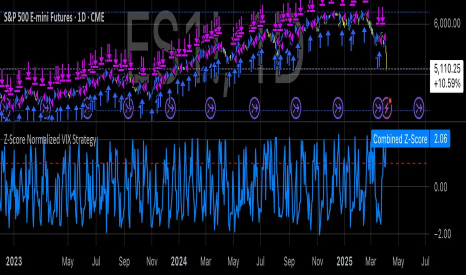
Z-Score Normalized VIX StrategyThis strategy leverages the concept of the Z-score applied to multiple VIX-based volatility indices, specifically designed to capture market reversals based on the normalization of volatility. The strategy takes advantage of VIX-related indicators to measure extreme levels of market fear or greed and adjusts its position accordingly.
1. Overview of the Z-Score Methodology
The Z-score is a statistical measure that describes the position of a value relative to the mean of a distribution in terms of standard deviations. In this strategy, the Z-score is calculated for various volatility indices to assess how far their values are from their historical averages, thus normalizing volatility levels. The Z-score is calculated as follows:
Z = \frac{X - \mu}{\sigma}
Where:
• X is the current value of the volatility index.
• \mu is the mean of the index over a specified period.
• \sigma is the standard deviation of the index over the same period.
This measure tells us how many standard deviations the current value of the index is away from its average, indicating whether the market is experiencing unusually high or low volatility (fear or calm).
2. VIX Indices Used in the Strategy
The strategy utilizes four commonly referenced volatility indices:
• VIX (CBOE Volatility Index): Measures the market’s expectations of 30-day volatility based on S&P 500 options.
• VIX3M (3-Month VIX): Reflects expectations of volatility over the next three months.
• VIX9D (9-Day VIX): Reflects shorter-term volatility expectations.
• VVIX (VIX of VIX): Measures the volatility of the VIX itself, indicating the level of uncertainty in the volatility index.
These indices provide a comprehensive view of the current volatility landscape across different time horizons.
3. Strategy Logic
The strategy follows a long entry condition and an exit condition based on the combined Z-score of the selected volatility indices:
• Long Entry Condition: The strategy enters a long position when the combined Z-score of the selected VIX indices falls below a user-defined threshold, indicating an abnormally low level of volatility (suggesting a potential market bottom and a bullish reversal). The threshold is set as a negative value (e.g., -1), where a more negative Z-score implies greater deviation below the mean.
• Exit Condition: The strategy exits the long position when the combined Z-score exceeds the threshold (i.e., when the market volatility increases above the threshold, indicating a shift in market sentiment and reduced likelihood of continued upward momentum).
4. User Inputs
• Z-Score Lookback Period: The user can adjust the lookback period for calculating the Z-score (e.g., 6 periods).
• Z-Score Threshold: A customizable threshold value to define when the market has reached an extreme volatility level, triggering entries and exits.
The strategy also allows users to select which VIX indices to use, with checkboxes to enable or disable each index in the calculation of the combined Z-score.
5. Trade Execution Parameters
• Initial Capital: The strategy assumes an initial capital of $20,000.
• Pyramiding: The strategy does not allow pyramiding (multiple positions in the same direction).
• Commission and Slippage: The commission is set at $0.05 per contract, and slippage is set at 1 tick.
6. Statistical Basis of the Z-Score Approach
The Z-score methodology is a standard technique in statistics and finance, commonly used in risk management and for identifying outliers or unusual events. According to Dumas, Fleming, and Whaley (1998), volatility indices like the VIX serve as a useful proxy for market sentiment, particularly during periods of high uncertainty. By calculating the Z-score, we normalize volatility and quantify the degree to which the current volatility deviates from historical norms, allowing for systematic entry and exit based on these deviations.
7. Implications of the Strategy
This strategy aims to exploit market conditions where volatility has deviated significantly from its historical mean. When the Z-score falls below the threshold, it suggests that the market has become excessively calm, potentially indicating an overreaction to past market events. Entering long positions under such conditions could capture market reversals as fear subsides and volatility normalizes. Conversely, when the Z-score rises above the threshold, it signals increased volatility, which could be indicative of a bearish shift in the market, prompting an exit from the position.
By applying this Z-score normalized approach, the strategy seeks to achieve more consistent entry and exit points by reducing reliance on subjective interpretation of market conditions.
8. Scientific Sources
• Dumas, B., Fleming, J., & Whaley, R. (1998). “Implied Volatility Functions: Empirical Tests”. The Journal of Finance, 53(6), 2059-2106. This paper discusses the use of volatility indices and their empirical behavior, providing context for volatility-based strategies.
• Black, F., & Scholes, M. (1973). “The Pricing of Options and Corporate Liabilities”. Journal of Political Economy, 81(3), 637-654. The original Black-Scholes model, which forms the basis for many volatility-related strategies.
Apex Trend SniperApex Trend Sniper - Advanced Trend Trading Strategy (Pine Script v5)
🚀 Overview
The Apex Trend Sniper is an advanced, fully automated trend-following strategy designed for crypto, forex, and stock markets. It combines momentum analysis, trend confirmation, volume validation, and adaptive risk management to capture high-probability trades. Unlike many strategies, this system is 100% non-repainting, ensuring reliable backtesting and real-time execution.
🔹 How This Strategy Works (Indicator Mashup)
The Apex Trend Sniper leverages multiple indicators to create a robust multi-layered confirmation system:
1️⃣ Trend Identification with RMI & McGinley Dynamic
📌 What It Does: Identifies the dominant trend and prevents trading against market conditions.
✔ McGinley Dynamic Baseline:
A highly adaptive moving average that dynamically reacts to price changes.
Price above the baseline = bullish trend.
Price below the baseline = bearish trend.
✔ Relative Momentum Index (RMI):
A refined Relative Strength Index (RSI) that filters out weak trends.
Above 50 = bullish confirmation.
Below 50 = bearish confirmation.
2️⃣ Trend Strength Confirmation with Vortex Indicator
📌 What It Does: Confirms that a detected trend is strong and valid.
✔ Vortex Indicator (VI):
Measures directional movement and trend strength.
A bullish trend is confirmed when VI+ > VI-.
A bearish trend is confirmed when VI- > VI+.
3️⃣ Volume Spike Detection for Trade Validation
📌 What It Does: Ensures that trades are placed only during strong market participation.
✔ Volume Confirmation:
A trade signal is only valid if volume spikes above the moving average.
Helps avoid false breakouts and weak trends.
4️⃣ Entry & Exit Strategy with Multi-Level Take Profits
📌 What It Does: Enters trades only when all conditions align and manages risk effectively.
✔ Entry Conditions (All must be met):
Price is above/below McGinley Dynamic.
RMI confirms trend direction.
Vortex indicator confirms trend strength.
Volume spike is detected.
✔ Exit Conditions:
Take Profit 1 (TP1): Secures 50% of the position at the first price target.
Take Profit 2 (TP2): Closes the remaining position at the second price target.
Exit Before Reversal: If an opposite trend signal appears, the position is closed early.
Trend Weakness Exit: If momentum weakens, the trade is exited automatically.
📌 Strategy Customization
🔧 Fully customizable to fit any trading style:
✔ McGinley Dynamic Length – Adjust baseline sensitivity.
✔ RMI & Vortex Settings – Fine-tune momentum filters.
✔ Volume Thresholds – Modify spike detection for better accuracy.
✔ Take Profit Levels – Set TP1 & TP2 based on market volatility.
📢 How to Use Apex Trend Sniper
1️⃣ Apply the strategy to any TradingView chart.
2️⃣ Customize the settings to fit your trading approach.
3️⃣ Use the backtest report to evaluate performance.
4️⃣ Monitor the dashboard to track real-time trade execution.
📌 Recommended Timeframes & Markets
✔ Best Markets:
✅ Crypto (BTC, ETH, SOL, etc.)
✅ Forex (EUR/USD, GBP/USD, JPY/USD, etc.)
✅ Stocks & Indices (S&P500, NASDAQ, etc.)
✔ Optimal Timeframes:
✅ Swing Trading: 1H – 4H – 1D
✅ Intraday & Scalping: 5M – 15M – 30M
📌 Backtest Settings for Realistic Performance
✔ Initial Capital: $1000 (or more for scaling).
✔ Commission: 0.05% (to simulate exchange fees).
✔ Slippage: 1-2 (to account for execution delay).
✔ Date Range: Test across different market conditions.
📢 TradingView Disclaimer
📌 This script is for educational purposes only and does not constitute financial advice. Trading carries significant risk, and past performance does not guarantee future results. Always test strategies thoroughly before applying them in a live market. Users are responsible for their own trading decisions.
🚀 Why Choose Apex Trend Sniper?
✅ Non-Repainting – No misleading signals.
✅ Multi-Layer Confirmation – Reduces false trades.
✅ Volume & Trend Strength Validation – Ensures high-probability entries.
✅ Adaptive Risk Management – Secures profits while maximizing trends.
✅ Versatile Across Markets & Timeframes – Works for crypto, forex, and stocks.
📢 Start Trading Smarter with Apex Trend Sniper! 🚀
🔗 Try it now on TradingView and optimize your trend-following strategy. 🔥

External Signals Strategy TesterExternal Signals Strategy Tester
This strategy is designed to help you backtest external buy/sell signals coming from another indicator on your chart. It is a flexible and powerful tool that allows you to simulate real trading based on signals generated by any indicator, using input.source connections.
🔧 How It Works
Instead of generating signals internally, this strategy listens to two external input sources:
One for buy signals
One for sell signals
These sources can be connected to the plots from another indicator (for example, custom indicators, signal lines, or logic-based plots).
To use this:
Add your indicator to the chart (it must be visible on the same pane as this strategy).
Open the settings of the strategy.
In the fields Buy Signal and Sell Signal, select the appropriate plot (line, value, etc.) from the indicator that represents the buy/sell logic.
The strategy will open positions when the selected buy signal crosses above 0, and sell signal crosses above 0.
This logic can be easily adapted by modifying the crossover rule inside the script if your signal style is different.
⚙️ Features Included
✅ Configurable trade direction:
You can choose whether to allow long trades, short trades, or both.
✅ Optional close on opposite signal:
When enabled, the strategy will exit the current position if an opposite signal appears.
✅ Optional full position reversal:
When enabled, the strategy will close the current position and immediately open an opposite one on the reverse signal.
✅ Risk Management Tools:
You can define:
Take Profit (TP): Position will be closed once the specified profit (in %) is reached.
Stop Loss (SL): Position will be closed if the price drops to the specified loss level (in %).
BreakEven (BE): Once the specified profit threshold is reached, the strategy will move the stop-loss to the entry price.
📌 If any of these values (TP, SL, BE) are set to 0, the feature is disabled and will not be applied.
🧪 Best Use Cases
Backtesting signals from custom indicators, without rewriting the logic into a strategy.
Comparing the performance of different signal sources.
Testing external indicators with optional position management logic.
Validating strategies using external filters, oscillators, or trend signals.
📌 Final Notes
You can visualize where the strategy detected buy/sell signals using green/red markers on the chart.
All parameters are customizable through the strategy settings panel.
This strategy does not repaint, and it processes signals in real-time only (no lookahead bias).

BTCUSD with adjustable sl,tpThis strategy is designed for swing traders who want to enter long positions on pullbacks after a short-term trend shift, while also allowing immediate short entries when conditions favor downside movement. It combines SMA crossovers, a fixed-percentage retracement entry, and adjustable risk management parameters for optimal trade execution.
Key Features:
✅ Trend Confirmation with SMA Crossover
The 10-period SMA crossing above the 25-period SMA signals a bullish trend shift.
The 10-period SMA crossing below the 25-period SMA signals a bearish trend shift.
Short trades are only taken if the price is below the 150 EMA, ensuring alignment with the broader trend.
📉 Long Pullback Entry Using Fixed Percentage Retracement
Instead of entering immediately on the SMA crossover, the strategy waits for a retracement before going long.
The pullback entry is defined as a percentage retracement from the recent high, allowing for an optimized entry price.
The retracement percentage is fully adjustable in the settings (default: 1%).
A dynamic support level is plotted on the chart to visualize the pullback entry zone.
📊 Short Entry Rules
If the SMA(10) crosses below the SMA(25) and price is below the 150 EMA, a short trade is immediately entered.
Risk Management & Exit Strategy:
🚀 Take Profit (TP) – Fully customizable profit target in points. (Default: 1000 points)
🛑 Stop Loss (SL) – Adjustable stop loss level in points. (Default: 250 points)
🔄 Break-Even (BE) – When price moves in favor by a set number of points, the stop loss is moved to break-even.
📌 Extra Exit Condition for Longs:
If the SMA(10) crosses below SMA(25) while the price is still below the EMA150, the strategy force-exits the long position to avoid reversals.
How to Use This Strategy:
Enable the strategy on your TradingView chart (recommended for stocks, forex, or indices).
Customize the settings – Adjust TP, SL, BE, and pullback percentage for your risk tolerance.
Observe the plotted retracement levels – When the price touches and bounces off the level, a long trade is triggered.
Let the strategy manage the trade – Break-even protection and take-profit logic will automatically execute.
Ideal Market Conditions:
✅ Trending Markets – The strategy works best when price follows strong trends.
✅ Stocks, Indices, or Forex – Can be applied across multiple asset classes.
✅ Medium-Term Holding Period – Suitable for swing trades lasting days to weeks.

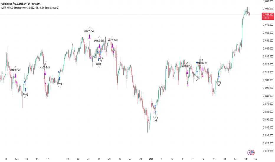
Multi-Timeframe MACD Strategy ver 1.0Multi-Timeframe MACD Strategy: Enhanced Trend Trading with Customizable Entry and Trailing Stop
This strategy utilizes the Moving Average Convergence Divergence (MACD) indicator across multiple timeframes to identify strong trends, generate precise entry and exit signals, and manage risk with an optional trailing stop loss. By combining the insights of both the current chart's timeframe and a user-defined higher timeframe, this strategy aims to improve trade accuracy, reduce exposure to false signals, and capture larger market moves.
Key Features:
Dual Timeframe Analysis: Calculates and analyzes the MACD on both the current chart's timeframe and a user-selected higher timeframe (e.g., Daily MACD on a 1-hour chart). This provides a broader market context, helping to confirm trends and filter out short-term noise.
Configurable MACD: Fine-tune the MACD calculation with adjustable Fast Length, Slow Length, and Signal Length parameters. Optimize the indicator's sensitivity to match your trading style and the volatility of the asset.
Flexible Entry Options: Choose between three distinct entry types:
Crossover: Enters trades when the MACD line crosses above (long) or below (short) the Signal line.
Zero Cross: Enters trades when the MACD line crosses above (long) or below (short) the zero line.
Both: Combines both Crossover and Zero Cross signals, providing more potential entry opportunities.
Independent Timeframe Control: Display and trade based on the current timeframe MACD, the higher timeframe MACD, or both. This allows you to focus on the information most relevant to your analysis.
Optional Trailing Stop Loss: Implements a configurable trailing stop loss to protect profits and limit potential losses. The trailing stop is adjusted dynamically as the price moves in your favor, based on a user-defined percentage.
No Repainting: Employs lookahead=barmerge.lookahead_off in the request.security() function to prevent data leakage and ensure accurate backtesting and real-time signals.
Clear Visual Signals (Optional): Includes optional plotting of the MACD and Signal lines for both timeframes, with distinct colors for easy visual identification. These plots are for visual confirmation and are not required for the strategy's logic.
Suitable for Various Trading Styles: Adaptable to swing trading, day trading, and trend-following strategies across diverse markets (stocks, forex, cryptocurrencies, etc.).
Fully Customizable: All parameters are adjustable, including timeframes, MACD Settings, Entry signal type and trailing stop settings.
How it Works:
MACD Calculation: The strategy calculates the MACD (using the standard formula) for both the current chart's timeframe and the specified higher timeframe.
Trend Identification: The relationship between the MACD line, Signal line, and zero line is used to determine the current trend for each timeframe.
Entry Signals: Buy/sell signals are generated based on the selected "Entry Type":
Crossover: A long signal is generated when the MACD line crosses above the Signal line, and both timeframes are in agreement (if both are enabled). A short signal is generated when the MACD line crosses below the Signal line, and both timeframes are in agreement.
Zero Cross: A long signal is generated when the MACD line crosses above the zero line, and both timeframes agree. A short signal is generated when the MACD line crosses below the zero line and both timeframes agree.
Both: Combines Crossover and Zero Cross signals.
Trailing Stop Loss (Optional): If enabled, a trailing stop loss is set at a specified percentage below (for long positions) or above (for short positions) the entry price. The stop-loss is automatically adjusted as the price moves favorably.
Exit Signals:
Without Trailing Stop: Positions are closed when the MACD signals reverse according to the selected "Entry Type" (e.g., a long position is closed when the MACD line crosses below the Signal line if using "Crossover" entries).
With Trailing Stop: Positions are closed if the price hits the trailing stop loss.
Backtesting and Optimization: The strategy automatically backtests on the chart's historical data, allowing you to assess its performance and optimize parameters for different assets and timeframes.
Example Use Cases:
Confirming Trend Strength: A trader on a 1-hour chart sees a bullish MACD crossover on the current timeframe. They check the MTF MACD strategy and see that the Daily MACD is also bullish, confirming the strength of the uptrend.
Filtering Noise: A trader using a 15-minute chart wants to avoid false signals from short-term volatility. They use the strategy with a 4-hour higher timeframe to filter out noise and only trade in the direction of the dominant trend.
Dynamic Risk Management: A trader enters a long position and enables the trailing stop loss. As the price rises, the trailing stop is automatically adjusted upwards, protecting profits. The trade is exited either when the MACD reverses or when the price hits the trailing stop.
Disclaimer:
The MACD is a lagging indicator and can produce false signals, especially in ranging markets. This strategy is for educational and informational purposes only and should not be considered financial advice. Backtest and optimize the strategy thoroughly, combine it with other technical analysis tools, and always implement sound risk management practices before using it with real capital. Past performance is not indicative of future results. Conduct your own due diligence and consider your risk tolerance before making any trading decisions.
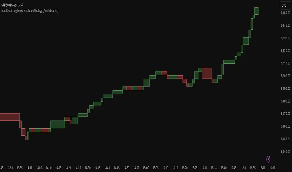
Non-Repainting Renko Emulation Strategy [PineIndicators]Introduction: The Repainting Problem in Renko Strategies
Renko charts are widely used in technical analysis for their ability to filter out market noise and emphasize price trends. Unlike traditional candlestick charts, which are based on fixed time intervals, Renko charts construct bricks only when price moves by a predefined amount. This makes them useful for trend identification while reducing small fluctuations.
However, Renko-based trading strategies often fail in live trading due to a fundamental issue: repainting .
Why Do Renko Strategies Repaint?
Most trading platforms, including TradingView, generate Renko charts retrospectively based on historical price data. This leads to the following issues:
Renko bricks can change or disappear when new data arrives.
Backtesting results do not reflect real market conditions. Strategies may appear highly profitable in backtests because historical data is recalculated with hindsight.
Live trading produces different results than backtesting. Traders cannot know in advance whether a new Renko brick will form until price moves far enough.
Objective of the Renko Emulator
This script simulates Renko behavior on a standard time-based chart without repainting. Instead of using TradingView’s built-in Renko charting, which recalculates past bricks, this approach ensures that once a Renko brick is formed, it remains unchanged .
Key benefits:
No past bricks are recalculated or removed.
Trading strategies can execute reliably without false signals.
Renko-based logic can be applied on a time-based chart.
How the Renko Emulator Works
1. Parameter Configuration & Initialization
The script defines key user inputs and variables:
brickSize : Defines the Renko brick size in price points, adjustable by the user.
renkoPrice : Stores the closing price of the last completed Renko brick.
prevRenkoPrice : Stores the price level of the previous Renko brick.
brickDir : Tracks the direction of Renko bricks (1 = up, -1 = down).
newBrick : A boolean flag that indicates whether a new Renko brick has been formed.
brickStart : Stores the bar index at which the current Renko brick started.
2. Identifying Renko Brick Formation Without Repainting
To ensure that the strategy does not repaint, Renko calculations are performed only on confirmed bars.
The script calculates the difference between the current price and the last Renko brick level.
If the absolute price difference meets or exceeds the brick size, a new Renko brick is formed.
The new Renko price level is updated based on the number of bricks that would fit within the price movement.
The direction (brickDir) is updated , and a flag ( newBrick ) is set to indicate that a new brick has been formed.
3. Visualizing Renko Bricks on a Time-Based Chart
Since TradingView does not support live Renko charts without repainting, the script uses graphical elements to draw Renko-style bricks on a standard chart.
Each time a new Renko brick forms, a colored rectangle (box) is drawn:
Green boxes → Represent bullish Renko bricks.
Red boxes → Represent bearish Renko bricks.
This allows traders to see Renko-like formations on a time-based chart, while ensuring that past bricks do not change.
Trading Strategy Implementation
Since the Renko emulator provides a stable price structure, it is possible to apply a consistent trading strategy that would otherwise fail on a traditional Renko chart.
1. Entry Conditions
A long trade is entered when:
The previous Renko brick was bearish .
The new Renko brick confirms an upward trend .
There is no existing long position .
A short trade is entered when:
The previous Renko brick was bullish .
The new Renko brick confirms a downward trend .
There is no existing short position .
2. Exit Conditions
Trades are closed when a trend reversal is detected:
Long trades are closed when a new bearish brick forms.
Short trades are closed when a new bullish brick forms.
Key Characteristics of This Approach
1. No Historical Recalculation
Once a Renko brick forms, it remains fixed and does not change.
Past price action does not shift based on future data.
2. Trading Strategies Operate Consistently
Since the Renko structure is stable, strategies can execute without unexpected changes in signals.
Live trading results align more closely with backtesting performance.
3. Allows Renko Analysis Without Switching Chart Types
Traders can apply Renko logic without leaving a standard time-based chart.
This enables integration with indicators that normally cannot be used on traditional Renko charts.
Considerations When Using This Strategy
Trade execution may be delayed compared to standard Renko charts. Since new bricks are only confirmed on closed bars, entries may occur slightly later.
Brick size selection is important. A smaller brickSize results in more frequent trades, while a larger brickSize reduces signals.
Conclusion
This Renko Emulation Strategy provides a method for using Renko-based trading strategies on a time-based chart without repainting. By ensuring that bricks do not change once formed, it allows traders to use stable Renko logic while avoiding the issues associated with traditional Renko charts.
This approach enables accurate backtesting and reliable live execution, making it suitable for trend-following and swing trading strategies that rely on Renko price action.
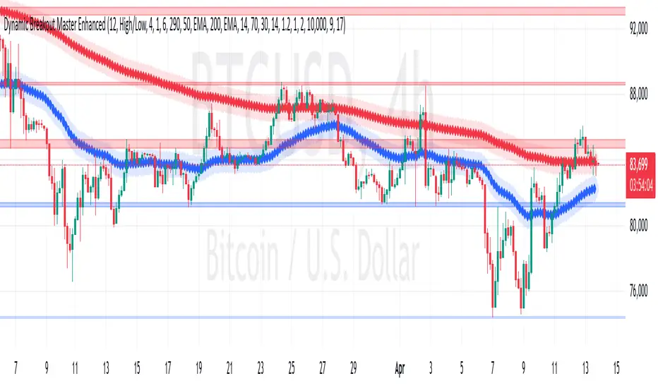
Dynamic Breakout Master by tradingbauhaus 🌟 Code Description:
This Pine Script implements a trading strategy called "Dynamic Breakout Master" 💥. The core idea of the strategy is to identify breakouts (price movements) at key support 💙 and resistance 🔴 levels, through a dynamic channel that adapts to the market’s conditions. Here's how it works:
🔧 Customizable Input Parameters:
🧭 Pivot Period: This defines the number of bars (candles) to the left and right used to detect pivots (highs and lows) that mark the support and resistance zones.
📊 Data Source: You can choose whether to use highs and lows or closes and opens of the candles to identify the pivots.
📏 Max Channel Width: Specifies the maximum width allowed for the support/resistance channel, expressed as a percentage over the last 300 bars.
💪 Minimum Pivot Strength: This defines the minimum number of pivots needed for a support or resistance level to be considered valid.
🏔 Max Support/Resistance Zones: Limits the number of key zones displayed on the chart.
📅 Lookback Period: Adjusts how many bars back the system should check to find and validate support and resistance levels.
🎨 Custom Colors: You can choose colors for the support, resistance, and in-channel zones.
📉 Moving Averages (MA): The strategy allows adding up to two moving averages (SMA or EMA) to assist in making trading decisions.
📊 Calculating Support/Resistance Levels:
The system uses an algorithm to identify pivots from prices and calculates dynamic support and resistance zones 🔒🔓.
The closer the pivots are and the stronger their influence, the more relevant the zone becomes for the strategy.
The dynamic channel is drawn on the chart, with a maximum width limit for these zones defined by the input parameter.
📈 Trading Logic:
🚀 Identifying Breakouts:
The strategy looks for when the price breaks (breakouts) a resistance or support level.
If the price breaks upward through the resistance level, a buy order 📈 is triggered.
If the price breaks downward through the support level, a sell order 📉 is triggered.
🔔 Alerts:
Resistance Break (ResBreak) and Support Break (SupBreak) alerts are configured to notify users when a significant breakout occurs.
💰 Commissions:
The strategy includes a commission (0.1%) to simulate transaction costs for each trade.
📊 Chart Visualization:
The support and resistance zones are displayed as colored rectangles:
🔴 Resistance (red) and
🔵 Support (blue).
Pivots of support and resistance can be labeled as P (for resistance) and V (for support).
Breakouts of support or resistance levels are marked with triangles that appear on the chart 🔺🔻.
📈 Trading Strategy:
If the price breaks upward through the resistance level, a long position (buy) 📈 is opened.
If the price breaks downward through the support level, a short position (sell) 📉 is opened.
🏆 Conclusion:
This script is a dynamic breakout strategy 💥 that allows traders to capture significant price movements when support or resistance channels break. The customizable parameters let users fine-tune the strategy according to their preferences, while the visual alerts on the chart make it easier to follow trading opportunities. The inclusion of moving averages and key price zones adds an extra layer of analysis to improve decision-making 💡.
Universal Strategy | QuantEdgeBIntroducing the Universal Strategy by QuantEdgeB
The Universal Strategy | QuantEdgeB is a dynamic, multi-indicator strategy designed to operate across various asset classes with precision and adaptability. This cutting-edge system utilizes four sophisticated methodologies, each integrating advanced trend-following, volatility filtering, and normalization techniques to provide robust signals. Its modular architecture and customizable features ensure suitability for diverse market conditions, empowering traders with data-driven decision-making tools. Its adaptability to different price behaviors and volatility levels makes it a robust and versatile tool, equipping traders with data-driven confidence in their market decisions.
_______
1. Core Methodologies and Features
1️⃣ DEMA ATR
Strength : Fast responsiveness to trend shifts.
The double exponential moving average is inherently aggressive, designed to reduce lag and quickly identify early signs of trend reversals or breakout opportunities. ATR bands add a volatility-sensitive layer, dynamically adjusting the breakout thresholds to match current market conditions, ensuring it remains responsive while filtering out noise
How It Fits :
This indicator is the first responder, providing early signals of potential trend shifts. While its aggressiveness can result in quick entries, it may occasionally overreact in noisy markets. This is where the smoother indicators step in to confirm signals.
2️⃣ Gaussian - VIDYA ATR (Variable Index Dynamic Average)
Strength : Smooth, adaptive trend identification.
Unlike DEMA, VIDYA adapts to market volatility through its standard deviation-based formula, making it smoother and less reactive to short-term fluctuations. ATR filtering ensures the indicator remains effective in volatile markets by dynamically adjusting its sensitivity.
How It Fits :
The smoother complement to DEMA ATR, VIDYA ATR filters out false signals from minor price movements. It provides confirmation for the trends identified by DEMA ATR, ensuring entries are based on robust, sustained price movements.
3️⃣ VIDYA Loop Trend Scoring
Strength : Historical trend scoring for consistent momentum detection.
This module evaluates the relative strength of trends by comparing the current VIDYA value to its historical values over a defined range. The loop mechanism provides a trend confidence score, quantifying the momentum behind price movements.
How It Fits :
VIDYA For-Loop adds a quantitative measure of trend strength, ensuring that trades are backed by sustained momentum. It balances the early signals from DEMA ATR and the smoothness of VIDYA ATR by providing a statistical check on the underlying trend.
4️⃣ Median SD with Normalization
Strength : Precision in breakout detection and market normalization.
The Median price serves as a robust baseline for detecting breakouts and reversals.
SD bands expand dynamically during periods of high volatility, making the indicator particularly effective for spotting strong trends or breakout opportunities. Normalization ensures the indicator adapts seamlessly across different assets and timeframes, providing consistent performance.
How It Fits :
The Median SD module provides final confirmation by focusing on price breakouts and market normalization. While the other indicators focus on momentum and trend strength, Median SD emphasizes precision, ensuring entries align with significant price movements rather than random fluctuations.
_______
2. How The Single Components Work Together
1️⃣ Balance of Speed and Smoothness :
The strategy blends quick responsiveness (DEMA ATR) with smooth and adaptive confirmation (VIDYA ATR & For-Loop), ensuring timely reactions without overreacting to market fluctuations. Median SD with Normalization refines breakout detection and stabilizes performance across assets using statistical anchors like price median and standard deviation.
Adaptability to Market Dynamics:
2️⃣ Adaptability to Market Dynamics :
The indicators complement each other seamlessly in trending markets, with the DEMA ATR and Median SD with Normalization quickly identifying shifts and confirming sustained momentum. In volatile or choppy markets, normalization and SD bands work together to filter out noise and reduce false signals, ensuring precise entries and exits. Meanwhile, the For-Loop scoring and Gaussian-Filtered VIDYA ATR focus on providing smoother, more reliable trend detection, offering consistent performance regardless of market conditions.
_______
3. Scoring and Signal Confirmation
The Universal Strategy consolidates signals from all four methodologies, calculating a Trend Probability Index (TPI). The four core indicators operate independently but contribute to a unified TPI, enabling highly adaptive behavior across asset classes.
- Each methodology generates a trend score: 1 for bullish trends, -1 for bearish trends.
- The TPI averages the scores, creating a unified signal.
- Long Position: Triggered when the TPI exceeds the long threshold (default: 0).
- Short Position: Triggered when the TPI falls below the short threshold (default: 0).
The strategy’s customizable settings allow traders to tailor its behavior to different market conditions—whether smoother trends in low-volatility assets or quick reaction to high-volatility breakouts. The long and short thresholds can be fine-tuned to match a trader’s risk tolerance and preferences.
_______
4. Use Cases:
The Universal Strategy | QuantEdgeB is designed to excel across a wide range of trading scenarios, thanks to its modular architecture and adaptability. Whether you're navigating trending, volatile, or range-bound markets, this strategy offers robust tools to enhance your decision-making. Below are the key use cases for its application:
1️⃣ Trend Trading
The strategy’s Gaussian-Filtered DEMA ATR and VIDYA ATR modules are perfect for identifying and riding sustained trends.
Ideal For: Traders looking to capture long-term momentum or position trades.
2️⃣ Breakout and Volatility-Based Strategies
With its Median SD with Normalization, the strategy excels in detecting volatility breakouts and significant price movements.
Ideal For: Traders aiming to capitalize on sudden market movements, especially in assets like cryptocurrencies and commodities.
3️⃣ Momentum and Strength Assessment
By generating a trend confidence score, the VIDYA For-Loop quantifies momentum strength—helping traders distinguish temporary spikes from sustainable trends.
Ideal For: Swing traders and those focusing on momentum-driven setups.
4️⃣ Adaptability Across Multiple Assets
The strategy’s robust framework ensures it performs consistently across different assets and timeframes.
Ideal For: Traders managing diverse portfolios or shifting between asset classes.
5️⃣ Backtesting and Optimization
Built-in backtesting and equity visualization tools make this strategy ideal for testing and refining parameters in real-world conditions.
• How It Helps: The strategy equity curve and metrics table offer a clear picture of performance, helping traders identify optimal settings for their chosen market and timeframe.
• Ideal For: Traders focused on rigorous testing and long-term optimization.
_______
5. Signal Composition Table:
This table presents a real-time breakdown of each indicator’s trend score (+1 bullish, -1 bearish) alongside the final aggregated signal. By visualizing the contribution of each methodology, traders gain greater transparency, confidence, and clarity in identifying long or short opportunities.
6. Customized Settings:
1️⃣ General Inputs
• Strategy Long Threshold (Lu): 0
• Strategy Short Threshold (Su): 0
2️⃣ Gaussian Filter
• Gaussian Length (len_FG): 4
• Gaussian Source (src_FG): close
• Gaussian Sigma (sigma_FG): 2.0
3️⃣ DEMA ATR
• DEMA Length (len_D): 30
• DEMA Source (src_D): close
• ATR Length (atr_D): 14
• ATR Multiplier (mult_D): 1.0
4️⃣ VIDYA ATR
• VIDYA Length (len_V1): 9
• SD Length (len_VHist1): 30
• ATR Length (atr_V): 14
• ATR Multiplier (mult_V): 1.7
5️⃣ VIDYA For-Loop
• VIDYA Length (len_V2): 2
• SD Length (len_VHist2): 5
• VIDYA Source (src_V2): close
• Start Loop (strat_loop): 1
• End Loop (end_loop): 60
• Long Threshold (long_t): 40
• Short Threshold (short_t): 8
6️⃣ Median SD
• Median Length (len_m): 24
• Normalized Median Length (len_msd): 50
• SD Length (SD_len): 32
• Long SD Weight (w1): 0.98
• Short SD Weight (w2): 1.02
• Long Normalized Smooth (smooth_long): 1
• Short Normalized Smooth (smooth_short): 1
Conclusion
The Universal Strategy | QuantEdgeB is a meticulously crafted, multi-dimensional trading system designed to thrive across diverse market conditions and asset classes. By combining Gaussian-Filtered DEMA ATR, VIDYA ATR, VIDYA For-Loop, and Median SD with Normalization, this strategy provides a seamless balance between speed, smoothness, and adaptability. Each component complements the others, ensuring traders benefit from early responsiveness, trend confirmation, momentum scoring, and breakout precision.
Its modular structure ensures versatility across trending, volatile, and consolidating markets. Whether applied to equities, forex, commodities, or crypto, it delivers data-driven precision while minimizing reliance on randomness, reinforcing confidence in decision-making.
With built-in backtesting tools, traders can rigorously evaluate performance under real-world conditions, while customization options allow fine-tuning for specific market dynamics and individual trading styles.
Why It Stands Out
The Universal Strategy | QuantEdgeB isn’t just a trading algorithm—it’s a comprehensive framework that empowers traders to make confident, informed decisions in the face of ever-changing market conditions. Its emphasis on precision, reliability, and transparency makes it a powerful tool for both professional and retail traders seeking consistent performance and enhanced risk management.
_______
🔹 Disclaimer: Past performance is not indicative of future results. No trading strategy can guarantee success in financial markets.
🔹 Strategic Advice: Always backtest, optimize, and align parameters with your trading objectives and risk tolerance before live trading.

Gold Pro StrategyHere’s the strategy description in a chat format:
---
**Gold (XAU/USD) Trend-Following Strategy**
This **trend-following strategy** is designed for trading gold (XAU/USD) by combining moving averages, MACD momentum indicators, and RSI filters to capture sustained trends while managing volatility risks. The strategy uses volatility-adjusted stops to protect gains and prevent overexposure during erratic price movements. The aim is to take advantage of trending markets by confirming momentum and ensuring entries are not made at extreme levels.
---
**Key Components**
1. **Trend Identification**
- **50 vs 200 EMA Crossover**
- **Bullish Trend:** 50 EMA crosses above 200 EMA, and the price closes above the 200 EMA
- **Bearish Trend:** 50 EMA crosses below 200 EMA, and the price closes below the 200 EMA
2. **Momentum Confirmation**
- **MACD (12,26,9)**
- **Buy Signal:** MACD line crosses above the signal line
- **Sell Signal:** MACD line crosses below the signal line
- **RSI (14 Period)**
- **Bullish Zone:** RSI between 50-70 to avoid overbought conditions
- **Bearish Zone:** RSI between 30-50 to avoid oversold conditions
3. **Entry Criteria**
- **Long Entry:** Bullish trend, MACD bullish crossover, and RSI between 50-70
- **Short Entry:** Bearish trend, MACD bearish crossover, and RSI between 30-50
4. **Exit & Risk Management**
- **ATR Trailing Stops (14 Period):**
- Initial Stop: 3x ATR from entry price
- Trailing Stop: Adjusts to lock in profits as price moves favorably
- **Position Sizing:** 100% of equity per trade (high-risk strategy)
---
**Key Logic Flow**
1. **Trend Filter:** Use the 50/200 EMA relationship to define the market's direction
2. **Momentum Confirmation:** Confirm trend momentum with MACD crossovers
3. **RSI Validation:** Ensure RSI is within non-extreme ranges before entering trades
4. **Volatility-Based Risk Management:** Use ATR stops to manage market volatility
---
**Visual Cues**
- **Blue Line:** 50 EMA
- **Red Line:** 200 EMA
- **Green Triangles:** Long entry signals
- **Red Triangles:** Short entry signals
---
**Strengths**
- **Clear Trend Focus:** Avoids counter-trend trades
- **RSI Filter:** Prevents entering overbought or oversold conditions
- **ATR Stops:** Adapts to gold’s inherent volatility
- **Simple Rules:** Easy to follow with minimal inputs
---
**Weaknesses & Risks**
- **Infrequent Signals:** 50/200 EMA crossovers are rare
- **Potential Missed Opportunities:** Strict RSI criteria may miss some valid trends
- **Aggressive Position Sizing:** 100% equity allocation can lead to large drawdowns
- **No Profit Targets:** Relies on trailing stops rather than defined exit targets
---
**Performance Profile**
| Metric | Expected Range |
|----------------------|---------------------|
| Annual Trades | 4-8 |
| Win Rate | 55-65% |
| Max Drawdown | 25-35% |
| Profit Factor | 1.8-2.5 |
---
**Optimization Recommendations**
1. **Increase Trade Frequency**
Adjust the EMAs to shorter periods:
- `emaFastLen = input.int(30, "Fast EMA")`
- `emaSlowLen = input.int(150, "Slow EMA")`
2. **Relax RSI Filters**
Adjust the RSI range to:
- `rsiBullish = rsi > 45 and rsi < 75`
- `rsiBearish = rsi < 55 and rsi > 25`
3. **Add Profit Targets**
Introduce a profit target at 1.5% above entry:
```pine
strategy.exit("Long Exit", "Long",
stop=longStopPrice,
profit=close*1.015, // 1.5% target
trail_offset=trailOffset)
```
4. **Reduce Position Sizing**
Risk a smaller percentage per trade:
- `default_qty_value=25`
---
**Best Use Case**
This strategy excels in **strong trending markets** such as gold rallies during economic or geopolitical crises. However, during sideways or choppy market conditions, the strategy might require manual intervention to avoid false signals. Additionally, integrating fundamental analysis—like monitoring USD weakness or geopolitical risks—can enhance its effectiveness.
---
This strategy offers a balanced approach for trading gold, combining trend-following principles with risk management tailored to the volatility of the market.

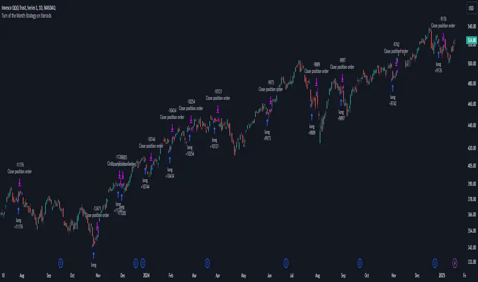
Turn of the Month Strategy on Steroids█ STRATEGY DESCRIPTION
The "Turn of the Month Strategy on Steroids" is a seasonal mean-reversion strategy designed to capitalize on price movements around the end of the month. It enters a long position when specific conditions are met and exits when the Relative Strength Index (RSI) indicates overbought conditions. This strategy is optimized for use on daily or higher timeframes.
█ WHAT IS THE TURN OF THE MONTH EFFECT?
The Turn of the Month effect refers to the observed tendency of stock prices to rise around the end of the month. This strategy leverages this phenomenon by entering long positions when the price shows signs of a reversal during this period.
█ SIGNAL GENERATION
1. LONG ENTRY
A Buy Signal is triggered when:
The current day of the month is greater than or equal to the specified `dayOfMonth` threshold (default is 25).
The close price is lower than the previous day's close (`close < close `).
The previous day's close is also lower than the close two days ago (`close < close `).
The signal occurs within the specified time window (between `Start Time` and `End Time`).
There is no existing open position (`strategy.position_size == 0`).
2. EXIT CONDITION
A Sell Signal is generated when the 2-period RSI exceeds 65, indicating overbought conditions. This prompts the strategy to exit the position.
█ ADDITIONAL SETTINGS
Day of Month: The day of the month threshold for triggering a Buy Signal. Default is 25.
Start Time and End Time: The time window during which the strategy is allowed to execute trades.
█ PERFORMANCE OVERVIEW
This strategy is designed to exploit seasonal price patterns around the end of the month.
It performs best in markets where the Turn of the Month effect is pronounced.
Backtesting results should be analyzed to optimize the `dayOfMonth` threshold and RSI parameters for specific instruments.
Systematic Risk Aggregation ModelThe “Systematic Risk Aggregation Model” is a quantitative trading strategy implemented in Pine Script™ designed to assess and visualize market risk by aggregating multiple financial risk factors. This model uses a multi-dimensional scoring approach to quantify systemic risk, incorporating volatility, drawdowns, put/call ratios, tail risk, volume spikes, and the Sharpe ratio. It derives a composite risk score, which is dynamically smoothed and plotted alongside adaptive Bollinger Bands to identify trading opportunities. The strategy’s theoretical framework aligns with modern portfolio theory and risk management literature (Markowitz, 1952; Taleb, 2007).
-----------------------------------------------------------------------------------------------
Key Components of the Model
1. Volatility as a Risk Proxy
The model calculates the standard deviation of the closing price over a specified period (volatility_length) to quantify market uncertainty. Volatility is normalized to a score between 0 and 100, using its historical minimum and maximum values.
Reference: Volatility has long been regarded as a critical measure of financial risk and uncertainty in capital markets (Hull, 2008).
2. Drawdown Assessment
The drawdown metric captures the relative distance of the current price from the highest price over the specified period (drawdown_length). This is converted into a normalized score to reflect the magnitude of recent losses.
Reference: Drawdown is a key metric in risk management, often used to measure potential downside risk in portfolios (Maginn et al., 2007).
3. Put/Call Ratio as a Sentiment Indicator
The strategy integrates the put/call ratio, sourced from an external symbol, to assess market sentiment. High values often indicate bearish sentiment, while low values suggest bullish sentiment (Whaley, 2000). The score is normalized similarly to other metrics.
4. Tail Risk via Modified Z-Score
Tail risk is approximated using the modified Z-score, which measures the deviation of the closing price from its moving average relative to its standard deviation. This approach captures extreme price movements and potential “black swan” events.
Reference: Taleb (2007) discusses the importance of considering tail risks in financial systems.
5. Volume Spikes as a Proxy for Market Activity
A volume spike is defined as the ratio of current volume to its moving average. This ratio is normalized into a score, reflecting unusual trading activity, which may signal market turning points.
Reference: Volume analysis is a foundational tool in technical analysis and is often linked to price momentum (Murphy, 1999).
6. Sharpe Ratio for Risk-Adjusted Returns
The Sharpe ratio measures the risk-adjusted return of the asset, using the mean log return divided by its standard deviation over the same period. This ratio is transformed into a score, reflecting the attractiveness of returns relative to risk.
Reference: Sharpe (1966) introduced the Sharpe ratio as a standard measure of portfolio performance.
----------------------------------------------------------------------------------------------
Composite Risk Score
The composite risk score is calculated as a weighted average of the individual risk factors:
• Volatility: 30%
• Drawdown: 20%
• Put/Call Ratio: 20%
• Tail Risk (Z-Score): 15%
• Volume Spike: 10%
• Sharpe Ratio: 5%
This aggregation captures the multi-dimensional nature of systemic risk and provides a unified measure of market conditions.
----------------------------------------------------------------------------------------------
Dynamic Bands with Bollinger Bands
The composite risk score is smoothed using a moving average and bounded by Bollinger Bands (basis ± 2 standard deviations). These bands provide dynamic thresholds for identifying overbought and oversold market conditions:
• Upper Band: Signals overbought conditions, where risk is elevated.
• Lower Band: Indicates oversold conditions, where risk subsides.
----------------------------------------------------------------------------------------------
Trading Strategy
The strategy operates on the following rules:
1. Entry Condition: Enter a long position when the risk score crosses above the upper Bollinger Band, indicating elevated market activity.
2. Exit Condition: Close the long position when the risk score drops below the lower Bollinger Band, signaling a reduction in risk.
These conditions are consistent with momentum-based strategies and adaptive risk control.
----------------------------------------------------------------------------------------------
Conclusion
This script exemplifies a systematic approach to risk aggregation, leveraging multiple dimensions of financial risk to create a robust trading strategy. By incorporating well-established risk metrics and sentiment indicators, the model offers a comprehensive view of market dynamics. Its adaptive framework makes it versatile for various market conditions, aligning with contemporary advancements in quantitative finance.
----------------------------------------------------------------------------------------------
References
1. Hull, J. C. (2008). Options, Futures, and Other Derivatives. Pearson Education.
2. Maginn, J. L., Tuttle, D. L., McLeavey, D. W., & Pinto, J. E. (2007). Managing Investment Portfolios: A Dynamic Process. Wiley.
3. Markowitz, H. (1952). Portfolio Selection. The Journal of Finance, 7(1), 77–91.
4. Murphy, J. J. (1999). Technical Analysis of the Financial Markets. New York Institute of Finance.
5. Sharpe, W. F. (1966). Mutual Fund Performance. The Journal of Business, 39(1), 119–138.
6. Taleb, N. N. (2007). The Black Swan: The Impact of the Highly Improbable. Random House.
7. Whaley, R. E. (2000). The Investor Fear Gauge. The Journal of Portfolio Management, 26(3), 12–17.

EMA Crossover Strategy with Take Profit and Candle HighlightingStrategy Overview:
This strategy is based on the Exponential Moving Averages (EMA), specifically the EMA 20 and EMA 50. It takes advantage of EMA crossovers to identify potential trend reversals and uses multiple take-profit levels and a stop-loss for risk management.
Key Components:
EMA Crossover Signals:
Buy Signal (Uptrend): A buy signal is generated when the EMA 20 crosses above the EMA 50, signaling the start of a potential uptrend.
Sell Signal (Downtrend): A sell signal is generated when the EMA 20 crosses below the EMA 50, signaling the start of a potential downtrend.
Take Profit Levels:
Once a buy or sell signal is triggered, the strategy calculates multiple take-profit levels based on the range of the previous candle. The user can define multipliers for each take-profit level.
Take Profit 1 (TP1): 50% of the previous candle's range above or below the entry price.
Take Profit 2 (TP2): 100% of the previous candle's range above or below the entry price.
Take Profit 3 (TP3): 150% of the previous candle's range above or below the entry price.
Take Profit 4 (TP4): 200% of the previous candle's range above or below the entry price.
These levels are adjusted dynamically based on the previous candle's high and low, so they adapt to changing market conditions.
Stop Loss:
A stop-loss is set to manage risk. The default stop-loss is 3% from the entry price, but this can be adjusted in the settings. The stop-loss is triggered if the price moves against the position by this amount.
Trend Direction Highlighting:
The strategy highlights the bars (candles) with colors:
Green bars indicate an uptrend (when EMA 20 crosses above EMA 50).
Red bars indicate a downtrend (when EMA 20 crosses below EMA 50).
These visual cues help users easily identify the market direction.
Strategy Entries and Exits:
Entries: The strategy enters a long (buy) position when the EMA 20 crosses above the EMA 50 and a short (sell) position when the EMA 20 crosses below the EMA 50.
Exits: The strategy exits the positions at any of the defined take-profit levels or the stop-loss. Multiple exit levels provide opportunities to take profit progressively as the price moves in the favorable direction.
Entry and Exit Conditions in Detail:
Buy Entry Condition (Uptrend):
A buy position is opened when EMA 20 crosses above EMA 50, signaling the start of an uptrend.
The strategy calculates take-profit levels above the entry price based on the previous bar's range (high-low) and the multipliers for TP1, TP2, TP3, and TP4.
Sell Entry Condition (Downtrend):
A sell position is opened when EMA 20 crosses below EMA 50, signaling the start of a downtrend.
The strategy calculates take-profit levels below the entry price, similarly based on the previous bar's range.
Exit Conditions:
Take Profit: The strategy attempts to exit the position at one of the take-profit levels (TP1, TP2, TP3, or TP4). If the price reaches any of these levels, the position is closed.
Stop Loss: The strategy also has a stop-loss set at a default value (3% below the entry for long trades, and 3% above for short trades). The stop-loss helps to protect the position from significant losses.
Backtesting and Performance Metrics:
The strategy can be backtested using TradingView's Strategy Tester. The results will show how the strategy would have performed historically, including key metrics like:
Net Profit
Max Drawdown
Win Rate
Profit Factor
Average Trade Duration
These performance metrics can help users assess the strategy's effectiveness over historical periods and optimize the input parameters (e.g., multipliers, stop-loss level).
Customization:
The strategy allows for the adjustment of several key input values via the settings panel:
Take Profit Multipliers: Users can customize the multipliers for each take-profit level (TP1, TP2, TP3, TP4).
Stop Loss Percentage: The user can also adjust the stop-loss percentage to a custom value.
EMA Periods: The default periods for the EMA 50 and EMA 20 are fixed, but they can be adjusted for different market conditions.
Pros of the Strategy:
EMA Crossover Strategy: A classic and well-known strategy used by traders to identify the start of new trends.
Multiple Take Profit Levels: By taking profits progressively at different levels, the strategy locks in gains as the price moves in favor of the position.
Clear Trend Identification: The use of green and red bars makes it visually easier to follow the market's direction.
Risk Management: The stop-loss and take-profit features help to manage risk and optimize profit-taking.
Cons of the Strategy:
Lagging Indicators: The strategy relies on EMAs, which are lagging indicators. This means that the strategy might enter trades after the trend has already started, leading to missed opportunities or less-than-ideal entry prices.
No Confirmation Indicators: The strategy purely depends on the crossover of two EMAs and does not use other confirming indicators (e.g., RSI, MACD), which might lead to false signals in volatile markets.
How to Use in Real-Time Trading:
Use for Backtesting: Initially, use this strategy in backtest mode to understand how it would have performed historically with your preferred settings.
Paper Trading: Once comfortable, you can use paper trading to test the strategy in real-time market conditions without risking real money.
Live Trading: After testing and optimizing the strategy, you can consider using it for live trading with proper risk management in place (e.g., starting with a small position size and adjusting parameters as needed).
Summary:
This strategy is designed to identify trend reversals using EMA crossovers, with customizable take-profit levels and a stop-loss to manage risk. It's well-suited for traders looking for a systematic way to enter and exit trades based on clear market signals, while also providing flexibility to adjust for different risk profiles and trading styles.
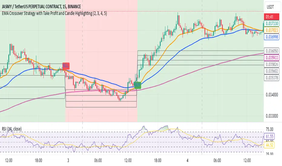
BullBear with Volume-Percentile TP - Strategy [presentTrading] Happy New Year, everyone! I hope we have a fantastic year ahead.
It's been a while since I published an open script, but it's time to return.
This strategy introduces an indicator called Bull Bear Power, combined with an advanced take-profit system, which is the main innovative and educational aspect of this script. I hope all of you find some useful insights here. Welcome to engage in meaningful exchanges. This is a versatile tool suitable for both novice and experienced traders.
█ Introduction and How it is Different
Unlike traditional strategies that rely solely on price or volume indicators, this approach combines Bull Bear Power (BBP) with volume percentile analysis to identify optimal entry and exit points. It features a dynamic take-profit mechanism based on ATR (Average True Range) multipliers adjusted by volume and percentile factors, ensuring adaptability to diverse market conditions. This multifaceted strategy not only improves signal accuracy but also optimizes risk management, distinguishing it from conventional trading methods.
BTCUSD 6hr performance
Disable the visualization of Bull Bear Power (BBP) to clearly view the Z-Score.
█ Strategy, How it Works: Detailed Explanation
The BBP Strategy with Volume-Percentile TP utilizes several interconnected components to analyze market data and generate trading signals. Here's an overview with essential equations:
🔶 Core Indicators and Calculations
1. Exponential Moving Average (EMA):
- **Purpose:** Smoothens price data to identify trends.
- **Formula:**
EMA_t = (Close_t * (2 / (lengthInput + 1))) + (EMA_(t-1) * (1 - (2 / (lengthInput + 1))))
- Usage: Baseline for Bull and Bear Power.
2. Bull and Bear Power:
- Bull Power: `BullPower = High_t - EMA_t`
- Bear Power: `BearPower = Low_t - EMA_t`
- BBP:** `BBP = BullPower + BearPower`
- Interpretation: Positive BBP indicates bullish strength, negative indicates bearish.
3. Z-Score Calculation:
- Purpose: Normalizes BBP to assess deviation from the mean.
- Formula:
Z-Score = (BBP_t - bbp_mean) / bbp_std
- Components:
- `bbp_mean` = SMA of BBP over `zLength` periods.
- `bbp_std` = Standard deviation of BBP over `zLength` periods.
- Usage: Identifies overbought or oversold conditions based on thresholds.
🔶 Volume Analysis
1. Volume Moving Average (`vol_sma`):
vol_sma = (Volume_1 + Volume_2 + ... + Volume_vol_period) / vol_period
2. Volume Multiplier (`vol_mult`):
vol_mult = Current Volume / vol_sma
- Thresholds:
- High Volume: `vol_mult > 2.0`
- Medium Volume: `1.5 < vol_mult ≤ 2.0`
- Low Volume: `1.0 < vol_mult ≤ 1.5`
🔶 Percentile Analysis
1. Percentile Calculation (`calcPercentile`):
Percentile = (Number of values ≤ Current Value / perc_period) * 100
2. Thresholds:
- High Percentile: >90%
- Medium Percentile: >80%
- Low Percentile: >70%
🔶 Dynamic Take-Profit Mechanism
1. ATR-Based Targets:
TP1 Price = Entry Price ± (ATR * atrMult1 * TP_Factor)
TP2 Price = Entry Price ± (ATR * atrMult2 * TP_Factor)
TP3 Price = Entry Price ± (ATR * atrMult3 * TP_Factor)
- ATR Calculation:
ATR_t = (True Range_1 + True Range_2 + ... + True Range_baseAtrLength) / baseAtrLength
2. Adjustment Factors:
TP_Factor = (vol_score + price_score) / 2
- **vol_score** and **price_score** are based on current volume and price percentiles.
Local performance
🔶 Entry and Exit Logic
1. Long Entry: If Z-Score crosses above 1.618, then Enter Long.
2. Short Entry: If Z-Score crosses below -1.618, then Enter Short.
3. Exiting Positions:
If Long and Z-Score crosses below 0:
Exit Long
If Short and Z-Score crosses above 0:
Exit Short
4. Take-Profit Execution:
- Set multiple exit orders at dynamically calculated TP levels based on ATR and adjusted by `TP_Factor`.
█ Trade Direction
The strategy determines trade direction using the Z-Score from the BBP indicator:
- Long Positions:
- Condition: Z-Score crosses above 1.618.
- Short Positions:
- Condition: Z-Score crosses below -1.618.
- Exiting Trades:
- Long Exit: Z-Score drops below 0.
- Short Exit: Z-Score rises above 0.
This approach aligns trades with prevailing market trends, increasing the likelihood of successful outcomes.
█ Usage
Implementing the BBP Strategy with Volume-Percentile TP in TradingView involves:
1. Adding the Strategy:
- Copy the Pine Script code.
- Paste it into TradingView's Pine Editor.
- Save and apply the strategy to your chart.
2. Configuring Settings:
- Adjust parameters like EMA length, Z-Score thresholds, ATR multipliers, volume periods, and percentile settings to match your trading preferences and asset behavior.
3. Backtesting:
- Use TradingView’s backtesting tools to evaluate historical performance.
- Analyze metrics such as profit factor, drawdown, and win rate.
4. Optimization:
- Fine-tune parameters based on backtesting results.
- Test across different assets and timeframes to enhance adaptability.
5. Deployment:
- Apply the strategy in a live trading environment.
- Continuously monitor and adjust settings as market conditions change.
█ Default Settings
The BBP Strategy with Volume-Percentile TP includes default parameters designed for balanced performance across various markets. Understanding these settings and their impact is essential for optimizing strategy performance:
Bull Bear Power Settings:
- EMA Length (`lengthInput`): 21
- **Effect:** Balances sensitivity and trend identification; shorter lengths respond quicker but may generate false signals.
- Z-Score Length (`zLength`): 252
- **Effect:** Long period for stable mean and standard deviation, reducing false signals but less responsive to recent changes.
- Z-Score Threshold (`zThreshold`): 1.618
- **Effect:** Higher threshold filters out weaker signals, focusing on significant market moves.
Take Profit Settings:
- Use Take Profit (`useTP`): Enabled (`true`)
- **Effect:** Activates dynamic profit-taking, enhancing profitability and risk management.
- ATR Period (`baseAtrLength`): 20
- **Effect:** Shorter period for sensitive volatility measurement, allowing tighter profit targets.
- ATR Multipliers:
- **Effect:** Define conservative to aggressive profit targets based on volatility.
- Position Sizes:
- **Effect:** Diversifies profit-taking across multiple levels, balancing risk and reward.
Volume Analysis Settings:
- Volume MA Period (`vol_period`): 100
- **Effect:** Longer period for stable volume average, reducing the impact of short-term spikes.
- Volume Multipliers:
- **Effect:** Determines volume conditions affecting take-profit adjustments.
- Volume Factors:
- **Effect:** Adjusts ATR multipliers based on volume strength.
Percentile Analysis Settings:
- Percentile Period (`perc_period`): 100
- **Effect:** Balances historical context with responsiveness to recent data.
- Percentile Thresholds:
- **Effect:** Defines price and volume percentile levels influencing take-profit adjustments.
- Percentile Factors:
- **Effect:** Modulates ATR multipliers based on price percentile strength.
Impact on Performance:
- EMA Length: Shorter EMAs increase sensitivity but may cause more false signals; longer EMAs provide stability but react slower to market changes.
- Z-Score Parameters:*Longer Z-Score periods create more stable signals, while higher thresholds reduce trade frequency but increase signal reliability.
- ATR Multipliers and Position Sizes: Higher multipliers allow for larger profit targets with increased risk, while diversified position sizes help in securing profits at multiple levels.
- Volume and Percentile Settings: These adjustments ensure that take-profit targets adapt to current market conditions, enhancing flexibility and performance across different volatility environments.
- Commission and Slippage: Accurate settings prevent overestimation of profitability and ensure the strategy remains viable after accounting for trading costs.
Conclusion
The BBP Strategy with Volume-Percentile TP offers a robust framework by combining BBP indicators with volume and percentile analyses. Its dynamic take-profit mechanism, tailored through ATR adjustments, ensures that traders can effectively capture profits while managing risks in varying market conditions.
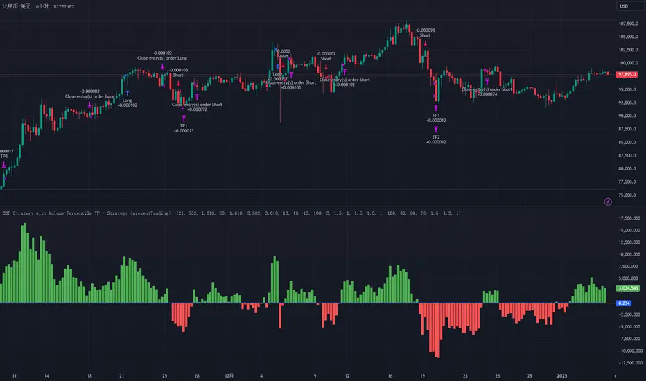
Kernel Regression Envelope with SMI OscillatorThis script combines the predictive capabilities of the **Nadaraya-Watson estimator**, implemented by the esteemed jdehorty (credit to him for his excellent work on the `KernelFunctions` library and the original Nadaraya-Watson Envelope indicator), with the confirmation strength of the **Stochastic Momentum Index (SMI)** to create a dynamic trend reversal strategy. The core idea is to identify potential overbought and oversold conditions using the Nadaraya-Watson Envelope and then confirm these signals with the SMI before entering a trade.
**Understanding the Nadaraya-Watson Envelope:**
The Nadaraya-Watson estimator is a non-parametric regression technique that essentially calculates a weighted average of past price data to estimate the current underlying trend. Unlike simple moving averages that give equal weight to all past data within a defined period, the Nadaraya-Watson estimator uses a **kernel function** (in this case, the Rational Quadratic Kernel) to assign weights. The key parameters influencing this estimation are:
* **Lookback Window (h):** This determines how many historical bars are considered for the estimation. A larger window results in a smoother estimation, while a smaller window makes it more reactive to recent price changes.
* **Relative Weighting (alpha):** This parameter controls the influence of different time frames in the estimation. Lower values emphasize longer-term price action, while higher values make the estimator more sensitive to shorter-term movements.
* **Start Regression at Bar (x\_0):** This allows you to exclude the potentially volatile initial bars of a chart from the calculation, leading to a more stable estimation.
The script calculates the Nadaraya-Watson estimation for the closing price (`yhat_close`), as well as the highs (`yhat_high`) and lows (`yhat_low`). The `yhat_close` is then used as the central trend line.
**Dynamic Envelope Bands with ATR:**
To identify potential entry and exit points around the Nadaraya-Watson estimation, the script uses **Average True Range (ATR)** to create dynamic envelope bands. ATR measures the volatility of the price. By multiplying the ATR by different factors (`nearFactor` and `farFactor`), we create multiple bands:
* **Near Bands:** These are closer to the Nadaraya-Watson estimation and are intended to identify potential immediate overbought or oversold zones.
* **Far Bands:** These are further away and can act as potential take-profit or stop-loss levels, representing more extreme price extensions.
The script calculates both near and far upper and lower bands, as well as an average between the near and far bands. This provides a nuanced view of potential support and resistance levels around the estimated trend.
**Confirming Reversals with the Stochastic Momentum Index (SMI):**
While the Nadaraya-Watson Envelope identifies potential overextended conditions, the **Stochastic Momentum Index (SMI)** is used to confirm a potential trend reversal. The SMI, unlike a traditional stochastic oscillator, oscillates around a zero line. It measures the location of the current closing price relative to the median of the high/low range over a specified period.
The script calculates the SMI on a **higher timeframe** (defined by the "Timeframe" input) to gain a broader perspective on the market momentum. This helps to filter out potential whipsaws and false signals that might occur on the current chart's timeframe. The SMI calculation involves:
* **%K Length:** The lookback period for calculating the highest high and lowest low.
* **%D Length:** The period for smoothing the relative range.
* **EMA Length:** The period for smoothing the SMI itself.
The script uses a double EMA for smoothing within the SMI calculation for added smoothness.
**How the Indicators Work Together in the Strategy:**
The strategy enters a long position when:
1. The closing price crosses below the **near lower band** of the Nadaraya-Watson Envelope, suggesting a potential oversold condition.
2. The SMI crosses above its EMA, indicating positive momentum.
3. The SMI value is below -50, further supporting the oversold idea on the higher timeframe.
Conversely, the strategy enters a short position when:
1. The closing price crosses above the **near upper band** of the Nadaraya-Watson Envelope, suggesting a potential overbought condition.
2. The SMI crosses below its EMA, indicating negative momentum.
3. The SMI value is above 50, further supporting the overbought idea on the higher timeframe.
Trades are closed when the price crosses the **far band** in the opposite direction of the trade. A stop-loss is also implemented based on a fixed value.
**In essence:** The Nadaraya-Watson Envelope identifies areas where the price might be deviating significantly from its estimated trend. The SMI, calculated on a higher timeframe, then acts as a confirmation signal, suggesting that the momentum is shifting in the direction of a potential reversal. The ATR-based bands provide dynamic entry and exit points based on the current volatility.
**How to Use the Script:**
1. **Apply the script to your chart.**
2. **Adjust the "Kernel Settings":**
* **Lookback Window (h):** Experiment with different values to find the smoothness that best suits the asset and timeframe you are trading. Lower values make the envelope more reactive, while higher values make it smoother.
* **Relative Weighting (alpha):** Adjust to control the influence of different timeframes on the Nadaraya-Watson estimation.
* **Start Regression at Bar (x\_0):** Increase this value if you want to exclude the initial, potentially volatile, bars from the calculation.
* **Stoploss:** Set your desired stop-loss value.
3. **Adjust the "SMI" settings:**
* **%K Length, %D Length, EMA Length:** These parameters control the sensitivity and smoothness of the SMI. Experiment to find settings that work well for your trading style.
* **Timeframe:** Select the higher timeframe you want to use for SMI confirmation.
4. **Adjust the "ATR Length" and "Near/Far ATR Factor":** These settings control the width and sensitivity of the envelope bands. Smaller ATR lengths make the bands more reactive to recent volatility.
5. **Customize the "Color Settings"** to your preference.
6. **Observe the plots:**
* The **Nadaraya-Watson Estimation (yhat)** line represents the estimated underlying trend.
* The **near and far upper and lower bands** visualize potential overbought and oversold zones based on the ATR.
* The **fill areas** highlight the regions between the near and far bands.
7. **Look for entry signals:** A long entry is considered when the price touches or crosses below the lower near band and the SMI confirms upward momentum. A short entry is considered when the price touches or crosses above the upper near band and the SMI confirms downward momentum.
8. **Manage your trades:** The script provides exit signals when the price crosses the far band. The fixed stop-loss will also close trades if the price moves against your position.
**Justification for Combining Nadaraya-Watson Envelope and SMI:**
The combination of the Nadaraya-Watson Envelope and the SMI provides a more robust approach to identifying potential trend reversals compared to using either indicator in isolation. The Nadaraya-Watson Envelope excels at identifying potential areas where the price is overextended relative to its recent history. However, relying solely on the envelope can lead to false signals, especially in choppy or volatile markets. By incorporating the SMI as a confirmation tool, we add a momentum filter that helps to validate the potential reversals signaled by the envelope. The higher timeframe SMI further helps to filter out noise and focus on more significant shifts in momentum. The ATR-based bands add a dynamic element to the entry and exit points, adapting to the current market volatility. This mashup aims to leverage the strengths of each indicator to create a more reliable trading strategy.

Moving Average Crossover Strategy with Take Profit and Stop LossThe Moving Average Crossover Strategy is a popular trading technique that utilizes two moving averages (MAs) of different periods to identify potential buy and sell signals. By incorporating take profit and stop loss levels, traders can effectively manage their risk while maximizing potential returns. Here’s a detailed explanation of how this strategy works:
Overview of the Moving Average Crossover Strategy
Moving Averages:
A short-term moving average (e.g., 50-day MA) reacts more quickly to price changes, while a long-term moving average (e.g., 200-day MA) smooths out price fluctuations over a longer period.
The strategy generates trading signals based on the crossover of these two averages:
Buy Signal: When the short-term MA crosses above the long-term MA (often referred to as a "Golden Cross").
Sell Signal: When the short-term MA crosses below the long-term MA (known as a "Death Cross").
Implementing Take Profit and Stop Loss
1. Setting Take Profit Levels
Definition: A take profit order automatically closes a trade when it reaches a specified profit level.
Strategy:
Determine a realistic profit target based on historical price action, support and resistance levels, or a fixed risk-reward ratio (e.g., 2:1).
For instance, if you enter a buy position at $100, you might set a take profit at $110 if you anticipate that level will act as resistance.
2. Setting Stop Loss Levels
Definition: A stop loss order limits potential losses by closing a trade when the price reaches a specified level.
Strategy:
Place the stop loss just below the most recent swing low for buy orders or above the recent swing high for sell orders.
Alternatively, you can use a percentage-based method (e.g., 2-3% below the entry point) to define your stop loss.
For example, if you enter a buy position at $100 with a stop loss set at $95, your maximum loss would be limited to $5 per share.
Example of Using Moving Average Crossover with Take Profit and Stop Loss
Entry Signal:
You observe that the 50-day MA crosses above the 200-day MA at $100. You enter a buy position.
Setting Take Profit and Stop Loss:
You analyze historical price levels and set your take profit at $110.
You place your stop loss at $95 based on recent swing lows.
Trade Management:
If the price rises to $110, your take profit order is executed, securing your profit.
If the price falls to $95, your stop loss is triggered, limiting your losses.
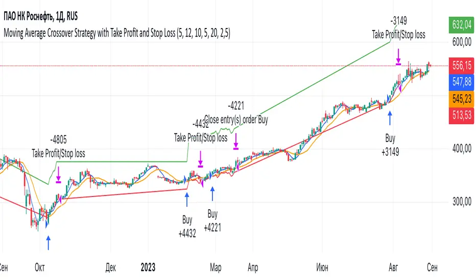
Trend Trader-Remastered StrategyOfficial Strategy for Trend Trader - Remastered
Indicator: Trend Trader-Remastered (TTR)
Overview:
The Trend Trader-Remastered is a refined and highly sophisticated implementation of the Parabolic SAR designed to create strategic buy and sell entry signals, alongside precision take profit and re-entry signals based on marked Bill Williams (BW) fractals. Built with a deep emphasis on clarity and accuracy, this indicator ensures that only relevant and meaningful signals are generated, eliminating any unnecessary entries or exits.
Please check the indicator details and updates via the link above.
Important Disclosure:
My primary objective is to provide realistic strategies and a code base for the TradingView Community. Therefore, the default settings of the strategy version of the indicator have been set to reflect realistic world trading scenarios and best practices.
Key Features:
Strategy execution date&time range.
Take Profit Reduction Rate: The percentage of progressive reduction on active position size for take profit signals.
Example:
TP Reduce: 10%
Entry Position Size: 100
TP1: 100 - 10 = 90
TP2: 90 - 9 = 81
Re-Entry When Rate: The percentage of position size on initial entry of the signal to determine re-entry.
Example:
RE When: 50%
Entry Position Size: 100
Re-Entry Condition: Active Position Size < 50
Re-Entry Fill Rate: The percentage of position size on initial entry of the signal to be completed.
Example:
RE Fill: 75%
Entry Position Size: 100
Active Position Size: 50
Re-Entry Order Size: 25
Final Active Position Size:75
Important: Even RE When condition is met, the active position size required to drop below RE Fill rate to trigger re-entry order.
Key Points:
'Process Orders on Close' is enabled as Take Profit and Re-Entry signals must be executed on candle close.
'Calculate on Every Tick' is enabled as entry signals are required to be executed within candle time.
'Initial Capital' has been set to 10,000 USD.
'Default Quantity Type' has been set to 'Percent of Equity'.
'Default Quantity' has been set to 10% as the best practice of investing 10% of the assets.
'Currency' has been set to USD.
'Commission Type' has been set to 'Commission Percent'
'Commission Value' has been set to 0.05% to reflect the most realistic results with a common taker fee value.
MACD Aggressive Scalp SimpleComment on the Script
Purpose and Structure:
The script is a scalping strategy based on the MACD indicator combined with EMA (50) as a trend filter.
It uses the MACD histogram's crossover/crossunder of zero to trigger entries and exits, allowing the trader to capitalize on short-term momentum shifts.
The use of strategy.close ensures that positions are closed when specified conditions are met, although adjustments were made to align with Pine Script version 6.
Strengths:
Simplicity and Clarity: The logic is straightforward and focuses on essential scalping principles (momentum-based entries and exits).
Visual Indicators: The plotted MACD line, signal line, and histogram columns provide clear visual feedback for the strategy's operation.
Trend Confirmation: Incorporating the EMA(50) as a trend filter helps avoid trades that go against the prevailing trend, reducing the likelihood of false signals.
Dynamic Exit Conditions: The conditional logic for closing positions based on weakening momentum (via MACD histogram change) is a good way to protect profits or minimize losses.
Potential Improvements:
Parameter Inputs:
Make the MACD (12, 26, 9) and EMA(50) values adjustable by the user through input statements for better customization during backtesting.
Example:
pine
Copy code
macdFast = input(12, title="MACD Fast Length")
macdSlow = input(26, title="MACD Slow Length")
macdSignal = input(9, title="MACD Signal Line Length")
emaLength = input(50, title="EMA Length")
Stop Loss and Take Profit:
The strategy currently lacks explicit stop-loss or take-profit levels, which are critical in a scalping strategy to manage risk and lock in profits.
ATR-based or fixed-percentage exits could be added for better control.
Position Size and Risk Management:
While the script uses 50% of equity per trade, additional options (e.g., fixed position sizes or risk-adjusted sizes) would be beneficial for flexibility.
Avoid Overlapping Signals:
Add logic to prevent overlapping signals (e.g., opening a new position immediately after closing one on the same bar).
Backtesting Optimization:
Consider adding labels or markers (label.new or plotshape) to visualize entry and exit points on the chart for better debugging and analysis.
The inclusion of performance metrics like max drawdown, Sharpe ratio, or profit factor would help assess the strategy's robustness during backtesting.
Compatibility with Live Trading:
The strategy could be further enhanced with alert conditions using alertcondition to notify the trader of buy/sell signals in real-time.

DCA Strategy with Mean Reversion and Bollinger BandDCA Strategy with Mean Reversion and Bollinger Band
The Dollar-Cost Averaging (DCA) Strategy with Mean Reversion and Bollinger Bands is a sophisticated trading strategy that combines the principles of DCA, mean reversion, and technical analysis using Bollinger Bands. This strategy aims to capitalize on market corrections by systematically entering positions during periods of price pullbacks and reversion to the mean.
Key Concepts and Principles
1. Dollar-Cost Averaging (DCA)
DCA is an investment strategy that involves regularly purchasing a fixed dollar amount of an asset, regardless of its price. The idea behind DCA is that by spreading out investments over time, the impact of market volatility is reduced, and investors can avoid making large investments at inopportune times. The strategy reduces the risk of buying all at once during a market high and can smooth out the cost of purchasing assets over time.
In the context of this strategy, the Investment Amount (USD) is set by the user and represents the amount of capital to be invested in each buy order. The strategy executes buy orders whenever the price crosses below the lower Bollinger Band, which suggests a potential market correction or pullback. This is an effective way to average the entry price and avoid the emotional pitfalls of trying to time the market perfectly.
2. Mean Reversion
Mean reversion is a concept that suggests prices will tend to return to their historical average or mean over time. In this strategy, mean reversion is implemented using the Bollinger Bands, which are based on a moving average and standard deviation. The lower band is considered a potential buy signal when the price crosses below it, indicating that the asset has become oversold or underpriced relative to its historical average. This triggers the DCA buy order.
Mean reversion strategies are popular because they exploit the natural tendency of prices to revert to their mean after experiencing extreme deviations, such as during market corrections or panic selling.
3. Bollinger Bands
Bollinger Bands are a technical analysis tool that consists of three lines:
Middle Band: The moving average, usually a 200-period Exponential Moving Average (EMA) in this strategy. This serves as the "mean" or baseline.
Upper Band: The middle band plus a certain number of standard deviations (multiplier). The upper band is used to identify overbought conditions.
Lower Band: The middle band minus a certain number of standard deviations (multiplier). The lower band is used to identify oversold conditions.
In this strategy, the Bollinger Bands are used to identify potential entry points for DCA trades. When the price crosses below the lower band, this is seen as a potential opportunity for mean reversion, suggesting that the asset may be oversold and could reverse back toward the middle band (the EMA). Conversely, when the price crosses above the upper band, it indicates overbought conditions and signals potential market exhaustion.
4. Time-Based Entry and Exit
The strategy has specific entry and exit points defined by time parameters:
Open Date: The date when the strategy begins opening positions.
Close Date: The date when all positions are closed.
This time-bound approach ensures that the strategy is active only during a specified window, which can be useful for testing specific market conditions or focusing on a particular time frame.
5. Position Sizing
Position sizing is determined by the Investment Amount (USD), which is the fixed amount to be invested in each buy order. The quantity of the asset to be purchased is calculated by dividing the investment amount by the current price of the asset (investment_amount / close). This ensures that the amount invested remains constant despite fluctuations in the asset's price.
6. Closing All Positions
The strategy includes an exit rule that closes all positions once the specified close date is reached. This allows for controlled exits and limits the exposure to market fluctuations beyond the strategy's timeframe.
7. Background Color Based on Price Relative to Bollinger Bands
The script uses the background color of the chart to provide visual feedback about the price's relationship with the Bollinger Bands:
Red background indicates the price is above the upper band, signaling overbought conditions.
Green background indicates the price is below the lower band, signaling oversold conditions.
This provides an easy-to-interpret visual cue for traders to assess the current market environment.
Postscript: Configuring Initial Capital for Backtesting
To ensure the backtest results align with the actual investment scenario, users must adjust the Initial Capital in the TradingView strategy properties. This is done by calculating the Initial Capital as the product of the Total Closed Trades and the Investment Amount (USD). For instance:
If the user is investing 100 USD per trade and has 10 closed trades, the Initial Capital should be set to 1,000 USD.
Similarly, if the user is investing 200 USD per trade and has 24 closed trades, the Initial Capital should be set to 4,800 USD.
This adjustment ensures that the backtesting results reflect the actual capital deployed in the strategy and provides an accurate representation of potential gains and losses.
Conclusion
The DCA strategy with Mean Reversion and Bollinger Bands is a systematic approach to investing that leverages the power of regular investments and technical analysis to reduce market timing risks. By combining DCA with the insights offered by Bollinger Bands and mean reversion, this strategy offers a structured way to navigate volatile markets while targeting favorable entry points. The clear entry and exit rules, coupled with time-based constraints, make it a robust and disciplined approach to long-term investing.
