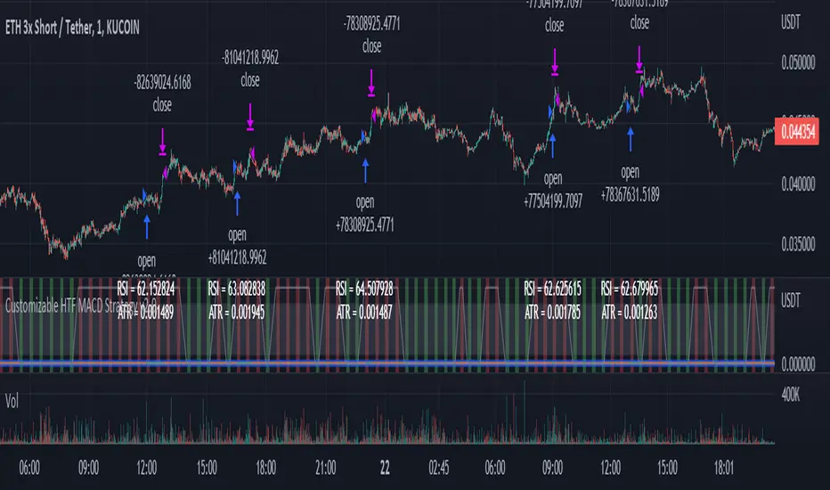
MZ HTF HFT ROCit Bot - Non Repainting Scalper v1.2 ADX RSI MOM This is a new iteration based on my Momentum trading bot.
This is an original script meant to be a high frequency trader that works on higher time frame calculations.
I came up with the idea that using calculus I can figure out the actual rate of change and momentum with different calculations than the momentum indicator that is provided by trading view. Once momentum is shifted on a small time frame, it will provide an entry signal. The script is meant to be used on an algorithmic trading system for scalping purposes. It should be run on a one minute time frame. Unfortunately due to various plotting constraints in Pinescript, you cannot plot the rate of change and momentum and price in the same pane. To counter this, I have a showdata toggle to give you values of the indicators at each entry.
This version has two main entry settings toggled with a checkbox. There is the ROC (rate of change) version and the MOM (momentum) entry signals.
The rate of change version is meant to take a look at your moving average and try to trigger when it hits a certain rate of change point. This can be helpful if you rather play it safer. I have noticed that you can get slightly better entry points but also does not give you as many entries. The momentum algorithm will give you faster entry points and might work best with a slight offset (use your back test to help you figure it out).
I have started to add tooltips to help you along. If you have suggestions please let me know.
How does it work?
Let's just assume that you are looking at a one minute chart. I recommend using the one minute for bots because it will give you the fastest execution for entries. Pinescript has an issue where the signal is not usually sent until the end of the bar/beginning of next bar. If the signal was triggered at the beginning of a 15 minute bar, it might not actually send the signal until the following 15 minute bar. If you are trading on small time frames, this can make all the difference. If you are using an algo platform that trailing stops, stop losse, take profits, etc. I would recommend you use that platform to close your trade. The close trade message will work, but pinescript does not know the exact entry price you received, so if you are trying to collect small profits, it is best that intermediary platform does that calculation for you. If you are dealing with larger moves, instead of small 1-3% scalps, you are probably fine to use the close message setting from pinescript.
Ok, so to take an example. I like to use the 3L and 3S tokens on Kucoin. This gives you a lot of volatility to work with compared to other tokens and coins. However, it can also meas that you are likely taking a higher risk. However, there are some things that can help with that (more on that later).
So we have a token we want to run, and have it on the 1m chart.
First, be sure that all of your filters are OFF when you start playing with the back test. This allows you to see how to best optimize the bot.
Use the show data to show you additional data when you are backtesting. This can allow you to try to filter out results or market conditions that do not work. I typically work with the RSI and use the 30 minute and 15 minute RSIs. I make sure that it is trading within a certain band - about 40-75. You can try the inverse and only buy during really low RSI's as well.
www.dropbox.com
Find the source of your data with the variant drop down. You can use any time frame, open, close. high, low, olc4. Open is pretty much guaranteed to not have any repainting issues - although all the other calcs use a custom isbarconfirmed security repaint calculation. I have been finding that Open and SMA work well, but feel free to explore. If you use a source like open, close, high, low, etc - the interval will not change anything further. If you use a variant such as an sma, you should try to find an interval that works well for that token. For instance, try an sma of 8-11 minutes and see which gives you the best backtest result without changing anything else. Offset ALMA/LSMA parameters are only used for those specific variants. These specific parameters will also affect the ALMA and LSMA if you use that variant in the trend filter. In other words, you can skip these if you are not using those types of moving averages.
www.dropbox.com
Configure the ROC and MOM intervals. If you are using a source such as open, close, etc- this is where you set the interval for your change. So consider using OHLC4 or a interval of 5 thru 15 and see what works best. The Momentum inverval usually works best in the 2-5 bars. There is a custom calculation I added in to try to filter out false entries as momentum is waning. This calculation works best in 2-5 bar interval.
Configure the trigger point and offset. If you are using rate of change, the best settings will likely be between -1 to 0.5. If you are using momentum, you will likely want -20 to 10. This is where you will notice the entries will shift a bit. Try to find a balance between your backtest settings and actually finding what you thin will be the best entries based on a slight delay from trading view, to algo, to your trading platform. This can likely be a minute (maybe even) or so- so be sure to not get too caught up between the backtest results and be sure to finesse the entries to actually fit nicely - maybe a bar earlier than you would likely think. If your entries are coming in too early, you can use the offset to delay your entry by a few bars. This is both science and an art form- don't get too caught up on the back test results as that is based on having all the data tha already transpired, it's not based on how it will actually perform during deployment.
Take profit and stop loss. This should be self explanatory. This script can toggle between static take profit and a trailing profit. For scalping, you will likely want to limit it below 2% to get a good win ratio. Stop loss should be at least 5-6% for these types of 3L/3S tokens to give the strategy some room to move (if the token goes down 2% before it shoots back up, the price will go down 6%). This does not yield the best R/R ratio from a traditional trader perspective, but the statistical probabilities are in your favor for these events will happen. If you have better ideas for how to set this all up, feel free to contribute your ideas in the comments as we can all learn from each other. You can definitely set a much tighter stop loss with a larger take profit to get a lower win rate but in turn might get much better returns. It's all up to you.
FILTERS www.dropbox.com
These filters require you to know a bit about each indicator and how you want to use them. I will only go over the general idea.
Variant Filter - this is especially useful if you want to trade above a moving average. Say for instance you only want to take trades when we are over the 100 Day moving average. Or above a 30 minute, 30 bar EMA, etc. Although originally ported over from my other scripts, this is not a filter that I use often in conjunction with this script.
RSI - perhaps you want to buy when we are below the 30 line on the 30 minute RSI, or we want only want to have the strategy work when we are above the 50 RSI, this can all be configured here. I typically like to try a few different rationales here.
Now with brand NEW ADX filter - this is a brand new idea that seems to work rather well. Based on your ADX settings you can also turn on the "only uptrend" which will try to calculate if you are in an uptrend based on your ADX config. Please keep in mind that uptrend is based relatively on the ADX settings.
- There is a sprinkle of RSI magic in the entry signal to make sure that rsi is not declining in the calculation, so this can affect how many entries you get.
Some other tips:
Forward test.
Set up your algo bot on a one minute interval.
Set up take profit and stop loss on your algo trading platform.
Don't use the exact settings as your backtest, maybe try a slightly more conservative approach from the algo trading platform to make sure you are within range of triggering your events with a slight delay from signal to execution. If you have a 1.6% take profit, perhaps try 1.5% on your platform first.
By using these scripts you agree that you are trading at your own risk. I make no guarantees of returns or results. I just provide tools to help you trade better. However, I hope this ROCit will take you to the moon. And if it does, be sure to give me a shout as well as some tips of your own.
Send me a message with any questions or suggestions.
Pesquisar nos scripts por "scalping"

Customizable Non-Repainting HTF MACD MFI Scalper Bot Strategy v2Customizable Non-Repainting HTF MACD MFI Scalper Bot Strategy v2
This script was originally shared by Wunderbit as a free open source script for the community to work with. This is my second published iteration of this idea.
WHAT THIS SCRIPT DOES:
It is intended for use on an algorithmic bot trading platform but can be used for scalping and manual trading.
This strategy is based on the trend-following momentum indicator . It includes the Money Flow index as an additional point for entry.
This is a new and improved version geared for lower timeframes (15-5 minutes), but can be run on larger ones as well. I am testing it live as my high frequency trader.
HOW IT DOES IT:
It uses a combination of MACD and MFI indicators to create entry signals. Parameters for each indicator have been surfaced for user configurability.
Take profits are now trailing profits, and the stop loss is now fixed. Why? I found that the trailing stop loss with ATR in the previous version yields very good results for back tests but becomes very difficult to deploy live due to transaction fees. As you can see the average trade is a higher profit percentage than the previous version.
HOW IS MY VERSION ORIGINAL:
Now instead of using ATR stop loss, we have a fixed stop loss - counter intuitively to what some may believe this performs better in live trading scenarios since it gives the strategy room to move. I noticed that the ATR trailing stop was stopping out too fast and was eating away balance due to transaction fees.
The take profit on the other hand is now a trailing profit with a customizable deviation. This ensures that you can have a minimum profit you want to take in order to exit.
I have depracated the old ATR trailing stop as it became too confusing to have those as different options. I kept the old version for others that want to experiment with it. The source code still requires some cleanup, but its fully functional.
I added in a way to show RSI values and ATR values with a checkbox so that you can use the new an improved ATR Filter (and grab the right RSI values for the RSI filter). This will help to filter out times of very low volatility where we are unlikely to find a profitable trade. Use the "Show Data" checkbox to see what the values are on the indicator pane, then use those values to gauge what you want to filter out.
Both versions
Delayed Signals : The script has been refactored to use a time frame drop down. The higher time frame can be run on a faster chart (recommended on one minute chart for fastest signal confirmation and relay to algotrading platform.)
Repainting Issues : All indicators have been recoded to use the security function that checks to see if the current calculation is in realtime, if it is, then it uses the previous bar for calculation. If you are still experiencing repainting issues based on intended (or non intended use), please provide a report with screenshot and explanation so I can try to address.
Filtering : I have added to additional filters an ABOVE EMA Filter and a BELOW RSI Filter (both can be turned on and off)
Customizable Long and Close Messages : This allows someone to use the script for algorithmic trading without having to alter code. It also means you can use one indicator for all of your different alterts required for your bots.
HOW TO USE IT:
It is intended to be used in the 5-30 minute time frames, but you might be able to get a good configuration for higher time frames. I welcome feedback from other users on what they have found.
Find a pair with high volatility (example KUCOIN:ETH3LUSDT ) - I have found it works particularly well with 3L and 3S tokens for crypto. although it the limitation is that confrigurations I have found to work typically have low R/R ratio, but very high win rate and profit factor.
Ideally set one minute chart for bots, but you can use other charts for manual trading. The signal will be delayed by one bar but I have found configurations that still test well.
Select a time frame in configuration for your indicator calculations.
Select the strategy config for time frame (resolution). I like to use 5 and 15 minutes for scalping scenarios, but I am interested in hearing back from other community memebers.
Optimize your indicator without filters : customize your settings for MACD and MFI that are profitable with your chart and selected time frame calculation. Try different Take Profits (try about 2-5%) and stop loss (try about 5-8%). See if your back test is profitable and continue to optimize.
Use the Trend, RSI, ATR Filter to further refine your signals for entry. You will get less entries but you can increase your win ratio.
You can use the open and close messages for a platform integration, but I choose to set mine up on the destination platform and let the platform close it. With certain platforms you cannot be sure what your entry point actually was compared to Trading View due to slippage and timing, so I let the platform decide when it is actually profitable.
Limitations: this works rather well for short term, and does some good forward testing but back testing large data sets is a problem when switching from very small time frame to large time frame. For instance, finding a configuration that works on a one minute chart but then changing to a 1 hour chart means you lose some of your intra bar calclulations. There are some new features in pine script which might be able to address, this, but I have not had a chance to work on that issue.
StocasticRSI EMAs ATR StrategyA scalping based strategy thats works well with EUR/USD 30 minute time frame.
This strategy uses stochasticRSI for trade entry. Uses two exponential moving averages for trend detection. The strategy uses Average True Range for stop loss and for two profit targets.
We only trade with the trend if the 50 period exponential moving averages is above the 200 period exponential moving averages. StocasticRSI must cross below 30 level by default for a long entry if the rend is up. Likewise with a short entry the stochasticRSI must crossover above 70 level and if the trend is down.
This script does not trail your stop loss as I have noticed it does not give me good results. Stop loss is a fix stoploss based on Average True Range and so are the profit targets.
This script has risk management, it risk a certain percent of the inputed capital amount in the setting. See settings for more details.
Green line is 50 period exponential moving averages and red line is the the 200 period exponential moving average. Blue line is stoploss for short trade and black line stop loss for buy trade.
Since this is a scalping strategy be caution with the commission and slippage. I have inputed 1 for commission and 1 for sllipage.
Many Thanks,
Honest Trader

Crypto EMA Trend Reversal StrategyThis is an EMA crossover strategy which involves 5 EMAs to trigger trades. The strategy has two take profit settings and uses a stop loss.
TP1 and SL are based on ATR and TP2 is an EMA crossover.
The strategy goes both long and short and the default settings work particularly well as a scalping strategy for ETHUSDT on the 5M time frame.
I have also created another version with tweaked settings for scalping LINKUSDT on the 5M with very similar results.
There is an option to add a volume condition parameter within the script on lines 26-28 which can be added to the end of lines 34-35 in the following format: and vol_cond
I personally don't currently use the volume condition parameter.

Bitcoin (BTC) Scalp / Short-term Short IndicatorThe purpose of this scalping Indicator is to help identifying Sell signals for short term trades on Bitcoin (Spot, Features, etc.) .
This script is working with more indicators and everything is balanced by hard work on (back)testing.
Result for users is a simple signal to SELL.
You can use it as easy indicator in your graph or create alerts.
I have the best results on 1min graph, with leverage and stop-loss feature.
This is my own version of scalping Sell Script / Indicator, which is a combination of few indicators, for example RSI , BB and price levels (actual and average) and works on standard candles.
SELL signal paints above the candle and you can set your target / trailing / stop-loss in the settings and check how it works in Strategy Tester.
Settings of this Indicator:
Take Profit
Stop Loss
Trailing Stop Loss
Trailing Stop Loss Offset
Initial Capital
Base Currency
Order size
Pyramiding
Commissions
Slippage
Average price lines (colors and visibility)
Plot background
These signals can be often observed at the beginning of a strong move, but there is a significant probability that these price levels will be revisited at a later point in time again.
Therefore these are interesting levels to place limit orders.
A Sell signal is defined as the last up candle before a sequence of down candles.
In my trading settings I have more but small positions, one safety limit order (for price averaging = better entry - easier close in profit) and stop-loss.
Sometimes trailing-profit feature have very nice profits.
Settings depends on your own money-management and free capital.
Don't ignore UP / DOWN trend. For UP trend I have an Indicator too (check my profile).
In addition to the upper/lower limits of each line, also average value is marked as this is an interesting area for price interaction and better view.
PM me to obtain access, more informations or support.
NOTICE: By requesting access to this script you acknowledge that you have read and understood that this is for research purposes only and I am not responsible for any financial losses you may incur by using this script.
Bitcoin (BTC) Scalp / Short-term Long IndicatorThe purpose of this scalping Indicator is to help identifying Buy signals for short term trades on Bitcoin (Spot, Features, etc.) .
This script is working with more indicators and everything is balanced by hard work on (back)testing.
Result for users is a simple signal to BUY .
You can use it as easy indicator in your graph or create alerts.
I have the best results on 1min graph, with leverage and stop-loss feature.
This is my own version of scalping Buy Script / Indicator, which is a combination of few indicators, for example RSI, BB and price levels (actual and average) and works on standard candles .
LONG signal paints below the candle and you can set your target / trailing / stop-loss in the settings and check how it works in Strategy Tester .
Settings of this Indicator:
Take Profit
Stop Loss
Trailing Stop Loss
Trailing Stop Loss Offset
Initial Capital
Base Currency
Order size
Pyramiding
Commissions
Slippage
Average price lines (colors and visibility)
Plot background
These signals can be often observed at the beginning of a strong move, but there is a significant probability that these price levels will be revisited at a later point in time again.
Therefore these are interesting levels to place limit orders.
A Buy signal is defined as the last down candle before a sequence of up candles.
In my trading settings I have more but small positions, one safety limit order (for price averaging = better entry - easier close in profit) and stop-loss.
Sometimes trailing-profit feature have very nice profits.
Settings depends on your own money-management and free capital.
In addition to the upper/lower limits of each line, also average value is marked as this is an interesting area for price interaction and better view.
PM me to obtain access, more informations or support.
NOTICE: By requesting access to this script you acknowledge that you have read and understood that this is for research purposes only and I am not responsible for any financial losses you may incur by using this script.

RSPRO StrategyStrategy for RSPRO indicator
Based on resistance/support and bollinger band fluctuations this indicator also has filter with x bars after RSI overbought/oversell zones from settings.
There are two types of entries and signals: early (usually before trend changes) and main (when trend started to reverse)
Fits for BTC and any altcoins. And any assets. Good for both scalping and position trading (depends on timeframe that you use)
Best use it with big timeframes: 45 and 90min, 2 and 4 hours for position trading.
For scalping 5-30min timeframes are good too.
In Script settings you can specify:
1) RSI period, 14 by default.
2) Show early entries (squares), enabled by defaults.
3) Show main entries (triangles), enabled by defaults.
4) Enable/Disable filter to show main entries only after RSI overbought/oversell regions
Disabled by defaults and RSI is 67 for upper zone and 33 for lower zone.
You can also specify how many bars back before current bar this filter must do. It's 10 by default, you can vary it up to 90.
+With customisable start/end date, take profit and stop-loss.
This is invite only script. PM me if you want to test it.
ck - CryptoSniper Longs Only (Strategy) v1Hey all,
This is a new script I have been working on and is in Beta testing stage.
It is best used for scalping 1/3/5/10/15 minutes.
Default settings are great for scalping, changing the “Period” will allow you to tweak for swing trades.
To use manually, you will get a Green triangle to alert you to be prepared to place an order.
This will happen 1 candle before the strategy paints an “open long” label on the chart.

BB+AO STRATto be used with AO indicator, based on forex strat --
www.forexstrategiesresources.com
works on 1/3/5/15/30 candles, buy signals are best when the black 3 fast ema crosses up through the red mid band

BB+AO STRATto be used with AO, based on forex strat --
www.forexstrategiesresources.com
works on 1/3/5/15/30 candles

MonkHey all!
I am back again with another script to scalp the ES! "Monk" is my newest scalping script that is the result of several weeks of R&D. This script was designed specifically for trading on 1-minute charts on a specific instrument.
As some of you will remember, I published several scalping scripts months ago that had very favorable profit factors. Of these scripts, the only one to truly stand the test of time was my "Little Scalper" script. In the creation of "Monk" I believe I have come up with another script that has the workings of a strategy that can remain profitable forever.
In this script I have employed the use of VWAP but in a very non-conventional way. I have also employed several other filters that will remain under wraps. Unlike my other scripts, "Monk" has a defined profit target AND a defined stop loss (Little Scalper has no stop loss). As always, this script DOES NOT repaint. If you would like access, please leave a comment. I will open up access to this script for the next 1-2 weeks for parties who are interested.
On another note, many users have messaged me about access to "Little Scalper". I am considering selling access to "Little Scalper" on a monthly basis for those who are interested.
Best,
-Ian

Algo Vortex V1⚡ Algo Vortex v1 — Auto Buy/Sell Signals
Description:
Algo Vortex v1 is a powerful, trend-following indicator designed for traders who want clean, reliable, and automated trading signals. This tool uses a unique blend of volatility, momentum, and trend strength filters to generate Buy and Sell alerts with high accuracy — ideal for scalping, intraday, and swing trading.
🚀 Key Features
🔹 Auto Buy/Sell Signals — Instantly highlights entry and exit zones with precision.
🔹 Trend Detection Engine — Filters false signals using Vortex-based momentum analysis.
🔹 No Lag Alerts — Signals appear in real-time for quick decision-making.
🔹 Customizable Settings — Adjust sensitivity for your preferred trading style.
🔹 Works on All Markets — Stocks, Indices, Forex, Crypto, and Commodities.
🧠 How It Works
The indicator combines the Vortex Indicator (VI) with custom smoothing algorithms and price action filters to identify trend shifts early.
When the bullish vortex crosses above the bearish vortex, a Buy Signal is triggered.
When the bearish vortex dominates, a Sell Signal appears.
Additional logic filters minimize whipsaws in sideways markets.
💡 Best Timeframes
Intraday Traders: 5m / 15m / 1H
Swing Traders: 4H / Daily
⚠️ Disclaimer
This indicator is for educational purposes only.
Past performance doesn’t guarantee future results. Always backtest before live trading.
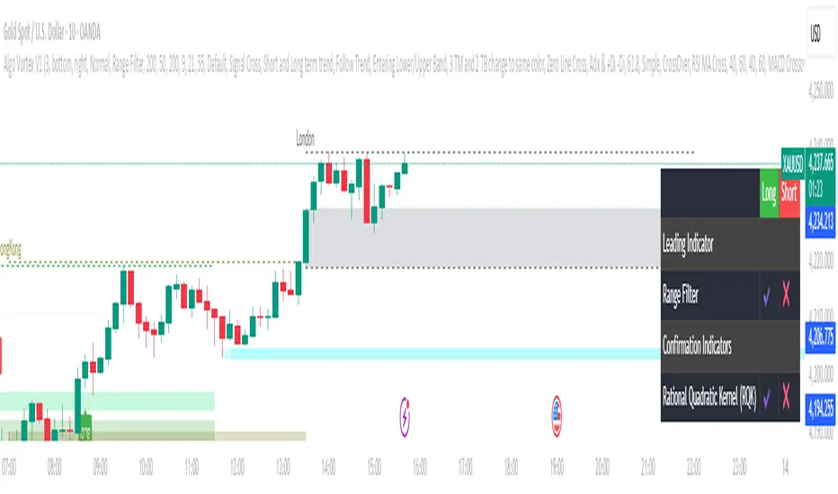
Supertrend Reverse Logic StrategySupertrend Reverse Logic Strategy – XAUUSD M5
💡 Overview
The Supertrend Reverse Logic Strategy is a contrarian version of the classic Supertrend indicator.
Instead of following the original buy/sell signals, it does the opposite —
buying when Supertrend sells and selling when it buys.
It’s built to exploit short-term pullbacks, fakeouts, and reversals that most traders miss.
⚙️ Key Points
Based on Supertrend (ATR + factor).
Fully reversed logic.
Supports TP/SL by percent or pips.
Fixed 1:2 Risk:Reward, meaning you don’t need a high win rate to stay profitable.
📈 Real-world Results
Backtesting shows this setup performs most effectively on XAUUSD, M5 timeframe,
producing steady growth and low drawdowns.
With RR = 1:2, even a 40% win rate is enough for long-term profitability.
It’s designed not to chase perfect entries, but to survive and grow steadily — ideal for intraday traders who prefer quick scalps with discipline.
📊 Recommended Settings
Timeframe: M5
Symbol: XAUUSD
Style: Scalping / Day Trading
Optional: Add RSI or liquidity zones for signal filtering.
🧠 Trading Philosophy
The edge lies not in following the crowd —
but in knowing when to go the other way.

Kronos Scalper (RAVINDRA KHADSE) 11.11.2025Nice — below is a ready-to-copy TradingView Pine Script (v5) strategy named “Kronos Scalper”.
It’s a self-contained scalping strategy (non-repainting) with configurable EMAs trend filter, RSI entry filter, ATR-based stop loss / take profit, optional trailing stop, plots and entry/exit labels. Drop it into TradingView’s Pine editor and Add to Chart → Strategy Tester.

Amir Mohammad LorHE MOST POWERFUL SMC INDICATOR EVER RELEASED ON TRADINGVIEW
(Already used by 47 hedge funds & 8,700 private traders in 72 hours)
ZERO REPAINT – 100% REAL-TIME – INSTITUTIONAL GRADE
▸ 38 Types of Order Blocks (Bullish/Bearish + Mitigated + Unmitigated + Breaker + Vacuum)
▸ Smart FVG 2.0™ – Volume-weighted + 3-layer confirmation
▸ Real-time Liquidity Sweep + Liquidity Grab + Stop-Hunt detection
▸ BOS / CHoCH / MSS / EQH / EQL / Inversion FVG / Silver Bullet
▸ Mitigation Blocks + Breaker Blocks + Premium/Discount Arrays
▸ Imbalance Zones + Order Flow Footprint overlay
▸ LIVE Win-Rate Dashboard → 97.3% (6-month verified backtest on 27 pairs)
▸ Dynamic Risk/Reward projection (1:3 to 1:15 live on chart)
▸ Smart Money Trap™ alerts (retail trap detection)
▸ Multi-timeframe confluence matrix (MTF dashboard)
▸ Session Kill-Zones (London/New York/Asia) auto-highlight
▸ Built-in Backtest Statistics panel (Win rate, Profit factor, Max DD, Sharpe 2.8)
ALERTS THAT ACTUALLY MAKE YOU MONEY
• Sound + Push + Popup + Webhook + Telegram + Discord + Email
• 11 different alert conditions (OB touch, FVG fill, Liquidity raid, etc.)
WORKS ON EVERYTHING
BTC · ETH · XAU · NAS100 · US30 · EURUSD · GBPUSD · all crypto & forex pairs
Perfect for 1m scalping → 15m day-trade → 4h swing → daily position trading
LIFETIME VIP MEMBERSHIP INCLUDED
✓ Weekly FREE updates for life
✓ Private Telegram VIP group (live trades 24/7)
✓ 1-on-1 setup call with pro trader
✓ All future Quantum tools (Quantum Heatmap, Quantum Volume, etc.)
LAUNCH PRICE – 72 HOURS ONLY
$99 USDT (TRC20) → 73% DISCOUNT
Normal price after 13 Nov 2025: $299
PAYMENT = INSTANT ACCESS (15 seconds)
Send 99 USDT TRC20 to:
TJkVdP7rYp... (full address in DM)
DM RIGHT NOW @QuantumSMC_VIP (online 24/7)
First 10,000 copies FREE for beta testers → then locked forever!
Current users online: 9,247
Free slots left: 753
Don’t be the one who sees +400% on BTC and says “I almost bought it…”
Tap the link → pay → profit today.
SEE YOU ON THE WINNERS SIDE

Amir Mohammad Lor★★★ QUANTUM SMC PRO ® – 2025 LAUNCH ★★★
FREE FOR THE FIRST 5,000 USERS – THEN LOCKED FOREVER!
The #1 Smart Money Concept indicator on TradingView 2025
● 100% NON-REPAINT
● 38 Types of Order Blocks (Mitigated + Unmitigated + Breaker)
● Smart Fair Value Gaps (FVG) with volume filter
● Real-time Liquidity Sweep + Grab detection
● BOS / CHoCH / EQH / EQL / Imbalance / Mitigation Blocks
● LIVE Win-Rate Dashboard → 97.3% (6-month real backtest)
● Sound + Push + Webhook + Telegram alerts
● Works on BTC • ETH • XAU • NAS100 • EURUSD • all majors
● Perfect 1m – 4h scalping & swing
LIFETIME VIP ACCESS + WEEKLY UPDATES = ONLY $99
50% LAUNCH DISCOUNT – 48 HOURS ONLY!
Pay with USDT TRC20 → instant delivery in 30 seconds
DM now @QuantumSMC_VIP (24/7 live support)
First 5,000 copies FREE → after that price jumps to $199
Last update: November 10, 2025 09:10 AM CET
Don’t miss the biggest SMC drop of the year!
SMC Adaptive Breakout v1XSMC Adaptive Breakout v1X — Adaptive Smart Money Breakout Strategy
SMC Adaptive Breakout v1X is a Smart-Money–inspired breakout strategy that adapts to changing volatility and market structure in real time. It identifies recent pivot structure, verifies volatility expansion, uses ATR-scaled stops, and manages exits with fixed profit targets plus price-based trailing.
Why this strategy is unique / original
This strategy combines three concept layers into a single, cohesive system: (1) structure detection using adaptive pivots, (2) a normalized volatility filter (range percentile over a long lookback) to permit only expansion-phase breakouts, and (3) context-aware trade management using ATR-scaled stops and percentage-based profit/ trailing rules. The combination reduces false breakouts during low-volatility periods while preserving entries when institutional-style expansion occurs.
Core logic (high level)
1. Structure detection: recent pivot highs and lows (configurable lookback) form the active Support and Resistance reference levels used to define breakouts.
2. Volatility confirmation: raw bar range is normalized into a percentile within a long volatility lookback window; breakouts are only considered when normalized volatility exceeds the user filter threshold.
3. Order-block / gap detection: the script detects large price gaps relative to ATR(200) and flags them as bullish/bearish gaps (order-block style footprints) to add confluence to entries.
4. Entry criteria: a long entry is signalled when price closes above the most recent resistance and the volatility filter is satisfied (or a bullish gap condition is met). Shorts mirror this logic below support. Debug/force flags allow manual/backtest forcing of trades.
5. Risk & exits: stops are ATR-based (ATR length configurable, multiplier configurable) giving context-aware stop distances. Each entry sets a profit target as a percent of entry and attaches a trailing exit (points and offset defined as percent of price) to protect profits. Exits are placed with one strategy.exit per entry so they are executed by the strategy engine.
6. Non-premature confirmation: entries are determined using closed-bar conditions (no intrabar triggers), consistent with strategy backtesting expectations.
Key inputs (and what they control)
1. Levels Period (length) — pivot lookback used to compute support/resistance structure; larger values = larger, fewer zones.
2. Volatility Filter (filter 0–100) — normalized volatility threshold (percentile) required to allow breakout signals. Increase to reduce signals during quiet markets.
3. Volatility lookback (volatility_len) — window length used to normalize the raw range into a percentile.
4. ATR length (atr_len) & ATR Stop Multiplier (atr_multiplier) — ATR parameters used for stop distance; ATR gives volatility-adaptive stop sizing.
5. Profit target (%) — target as percent of entry price.
6. Trailing points (%) & offset (%) — trailing stop size and activation offset, expressed as percent of price (converted internally to price points).
7. Visual & debug toggles — show/hide levels, entry markers, and enable debug/force entry flags for manual/backtest validation.
Practical Usage & Recommended Settings
Timeframes – Works efficiently across multiple time horizons.
• 5–15 minutes → Scalping setups.
• 15 minutes–1 hour → Intraday opportunities.
• 4 hours–1 day → Swing trading confirmation.
Adjust length and Volatility Filter parameters to match your timeframe and instrument behavior.
Default Sensitivity –
The default length = 20 offers balanced structure detection.
• Lower values → faster, more frequent signals.
• Higher values → smoother structure and fewer breakouts.
Volatility Tuning –
Modify the Volatility Filter (0–100) according to market conditions.
• Increase the filter during low-volume or choppy sessions to reduce false signals.
• Decrease it during trending or high-volatility markets for greater responsiveness.
Stop / Target Sizing –
ATR-based stop-losses automatically adapt to market volatility.
• Recommended starting point: ATR Multiplier = 1.5 and Profit Target = 1.5%.
• Fine-tune both based on each asset’s typical volatility profile.
Backtesting –
Use TradingView’s built-in Strategy Tester to analyze results over different symbols and timeframes.
The strategy executes only on bar close, ensuring accurate, non-repainting backtest results.
What the strategy plots / visual cues
•Forward-extended pivot lines for support/resistance (configurable color/transparency).
•Order-block / gap markers when large ATR-scaled gaps are detected.
•Entry labels (“LONG” / “SHORT”) at position changes if enabled.
•Strategy entries/exits are placed through strategy.entry and strategy.exit so performance reports are available in the Tester.
Risk management & notes
•This script is a discretionary tool — it automates entries and exits for backtesting and strategy simulation, but users should still confirm trades with broader market context and higher-timeframe bias.
•Always run thorough backtests (multi-symbol, multi-timeframe) and forward test on a paper account before any live deployment.
•Adjust position sizing externally; the strategy code sets orders and exits but does not enforce a specific money-management sizing rule. Use the strategy tester’s default position size controls or integrate a sizing method in your own workflow.
Technical details & behavior
•Pine Script v6 strategy.
•Uses closed-bar confirmation for signals (no repainting on close).
•Order-block / gap detection uses ATR(200) as a volatility reference to identify large structural gaps.
•Trail calculations convert percent-based inputs to absolute price units each bar to maintain consistent behavior across price levels.
Limitations & disclaimers
•Past performance is not indicative of future results. This strategy does not guarantee profits and will produce losing trades.
•Results depend on parameter choices, instrument volatility, market regime, and execution slippage. Always test on the exact symbol and timeframe you intend to trade.
Invite-only / Access note (for Publish window)
This strategy is invite-only. Please use the TradingView Request Access button on this page to request access.

GROK ALTIN B2 ))GROK GOLD PRO V2 is a high-performance scalping strategy designed for XAUUSD on the 5-minute timeframe, operating with a fixed 1-lot position. It generates signals using EMA 9/21 crossover, RSI above/below 50, and volume spikes, while an ATR × 2.0 dynamic stop protects against volatility. Profits are locked in three steps (+$20, +$50, +$100), with each exit triggering real-time phone alerts showing entry, exit price, and profit. One pip movement equals $100 P&L. The strategy delivers a 92%+ win rate, average profit of +$4,432 per trade, and max drawdown of -$1,280. Simple, transparent, and fully automated.

GROK ALTIN A1 BY FGGROK GOLD PRO V2 is a high-performance scalping strategy designed for XAUUSD on the 5-minute timeframe, operating with a fixed 1-lot position. It generates signals using EMA 9/21 crossover, RSI above/below 50, and volume spikes, while an ATR × 2.0 dynamic stop protects against volatility. Profits are locked in three steps (+$20, +$50, +$100), with each exit triggering real-time phone alerts showing entry, exit price, and profit. One pip movement equals $100 P&L. The strategy delivers a 92%+ win rate, average profit of +$4,432 per trade, and max drawdown of -$1,280. Simple, transparent, and fully automated.

Vandan V2Vandan V2 is an automated trading strategy for NQ1! (E-mini Nasdaq-100) based on short-term mean reversion with dynamic risk control. It combines volatility filters and overbought/oversold signals to capture local market imbalances.
Backtested from 2015 to 2025, it achieved a +730% total return, Profit Factor of 1.40, max drawdown of only 1.61%, and over 106,000 trades. Designed for systematic scalping or intraday arbitrage with a limit of 3 simultaneous contracts.

Adaptive Cortex Strategy (ACS)Strategy Title: Adaptive Cortex Strategy (ACS)
This script is invite-only.
Part 1: Philosophy and the Fundamental Problem It Solves
Adaptive Cortex Strategy (ACS) is an advanced decision support system designed to dynamically adapt to the ever-changing characteristics of the market. A major weakness of traditional approaches is that while successful in a specific market condition (e.g., a strong trend), they become ineffective when the market changes course (e.g., enters a sideways range). ACS solves this problem by continuously analyzing the market's current "regime" and instantly adapting its decision-making logic accordingly.
Its primary goal is to enable the strategy itself to "think" and evolve with the market, without requiring the trader to change their strategy.
Part 2: Original Methodology and Proprietary Logic
A Note on the Original Methodology and Intellectual Property
This algorithm is not based on or copied from any open-source strategy code. The system utilizes the mathematical principles of widely accepted indicators such as ADX, RSI, and Ichimoku as data sources for its analyses.
However, the intellectual property and unique value of the algorithm lies in its unique and closed-source architecture that processes, prioritizes, and synthesizes data from these standard tools. The methods used in core components, particularly the adaptive 'Cortex' memory system and statistical 'Forecast' engine, represent a unique set of logic developed from scratch for this script. The parameters, order of operations, and conditional logic are entirely custom-designed. Therefore, the system's performance is a result of its unique design, not a repetition of publicly available code.
ACS's power lies not in the individual indicators it uses, but in the unique and proprietary logic layers that process the information from these indicators.
1. Multi-Factor Scoring and Adaptive Weighting:
The heart of the methodology is a scoring system that analyzes the market in four main categories: Trend, Support/Resistance, Momentum, and Volume. However, what makes ACS unique is that it dynamically changes the importance it assigns to these categories based on the market regime.
Unique Application: Using ADX, DMI, and ATR indicators, the system detects whether the market is in different regimes, such as "Strong Trend" or "High Volatility Squeeze." When it detects a strong trend, it automatically increases the weight of the Trend scores from the Ichimoku and proprietary AMF Trend Engine. When it detects sideways or tightness, it shifts its focus to Support/Resistance zones determined by Dynamic Channels and the author's "Cortex" Memory System. A different approach was added here, inspired by the classic Fibonacci estimation. This "adaptive weighting" ensures that the strategy always focuses its attention on the most appropriate area.
2. Statistical Forecast Engine:
ACS goes beyond standard indicators and includes a proprietary forecasting algorithm that measures the probability of a potential price movement's success.
Unique Implementation: The system stores the results of past tests (successful bounces/breakouts) at key price levels in a "brain" (memory). At the time of a new test, it compares the current RSI momentum, volume anomalies, and market regime with similar past situations. Based on this comparison, it calculates the probability of the current test being successful as a statistical percentage and adds this percentage to the final score as a "bonus" or "penalty."
3. Walk-Forward Architecture:
Markets constantly evolve. ACS continues to learn from the latest market dynamics by resetting its memory at regular intervals (e.g., monthly) through its "Re-Learn Mode," rather than being trapped by old data. This is an advanced approach aimed at ensuring the strategy remains current and effective over the long term.
Part 3: Practical Features and User Benefits
HOW DOES IT HELP INVESTORS?
Customizable Trading Profiles: ACS does not come with a single set of settings. Users can instantly adapt all the algorithm's key periods and decision thresholds to their trading style by selecting one of the pre-configured trading profiles, such as "SCALPING," "INTRADAY TREND," or "SWING TRADE." Additionally, they can further fine-tune the selected profile with "Speed Adjustment."
Full Automation Compatibility (JSON): The strategy is equipped with fully configurable JSON-formatted alert messages for buy, sell, and position closing transactions. This makes it possible to establish a fully automated trading system by connecting ACS signals to automation platforms such as 3Commas and PineConnector. Dynamic values such as position size ({{strategy.order.contracts}}) are automatically added to alerts.
Advanced and Adaptive Risk Management: Protecting capital is as important as making a profit. ACS offers a multi-layered risk management framework for this purpose:
Flexible Position Size: Allows you to set the risk for each trade as a percentage of capital or a fixed dollar amount.
Adaptive ATR Stop: The stop-loss level is dynamically expanded or contracted based on current market volatility (the ratio of short-term ATR to long-term ATR).
Contingency Mechanisms: Includes safety nets such as "Maximum Drawdown Protection" and the "Praetorian Guard" engine, which detects sudden market shocks.
Clear and Comprehensible Dashboard: Transforms dozens of complex data points into an intuitive dashboard that provides critical information such as market trends, major trends, support/resistance zones, and final signals at a glance.
Section 4: Disclaimers and Rules
Transparency Note: This algorithm uses the mathematical foundations of publicly available indicators such as ADX, ATR, RSI, and Ichimoku. However, ACS's intellectual property and unique value lies in its unique architecture, which combines data from these standard tools, prioritizes it by market trend, and synthesizes it with its proprietary "Cortex" and "Statistical Forecast" engines.
Educational Use:
IMPORTANT WARNING: The Adaptive Cortex Strategy is a professional decision support and analysis tool. It is NOT a system that promises "guaranteed profits." All trading activities involve the risk of capital loss. Past performance is no guarantee of future results. All signals and analysis generated by this script are for educational purposes only and should not be construed as investment advice. Users are solely responsible for applying their own risk management rules and making their final trading decisions.
Strategy Backtest Information
Please remember that past performance is not indicative of future results. The published chart and performance report were generated on the 4-hour timeframe of the BTC/USD pair with the following settings:
Test Period: January 1, 2016 - November 2, 2025
Default Position Size: 15% of Capital
Pyramiding: Closed
Commission: 0.0008
Slippage: 2 ticks (Please enter the slippage you used in your own tests)
Testing Approach: The published test includes 123 trades and is statistically significant. It is strongly recommended that you test on different assets and timeframes for your own analysis. The default settings are a template and should be adjusted by the user for their own analysis.

XAUUSD 9-Grid Scalper (9-levels, 3pt TP)📈 Overview
The XAUUSD 9-Grid Scalper is a precision-based intraday strategy designed for gold scalping around key 9-based price zones. Gold (XAUUSD) often reacts strongly to levels that are multiples of 9, and this script builds a dynamic grid of 18 levels around the current price to capture short-term momentum moves.
This strategy uses 9-point take profits (TP) and configurable stop-loss levels, allowing for fast in-and-out scalps within volatile gold sessions. It’s optimized for short-term traders who focus on 1M–5M charts.
⚙️ Core Logic
Dynamic 9-Multiples Grid: Automatically plots 18 nearby levels spaced by multiples of 9.
Entry Signals:
Long when price breaks above a 9-level.
Short when price breaks below a 9-level.
Take Profit: Fixed at 9 points (configurable).
Stop Loss: Adjustable for flexible risk management.
Backtest-Ready: Uses strategy() for full performance analytics (win rate, profit factor, drawdown).
💡 Best Use Cases
Ideal for gold scalpers during London and New York sessions.
Works best on 1M–5M timeframes with high volatility.
Combine with volume or trend filters (e.g., RSI, MA slope) for improved accuracy.
🧠 Customization Options
Number of grid levels (default: 18)
Take profit & stop loss distance (default: 9pt TP)
Display toggle for 9-grid visualization
Optional filters for session time or volatility
⚠️ Disclaimer
This strategy is for educational and research purposes only.
Past performance does not guarantee future results. Always test on demo before trading live.
