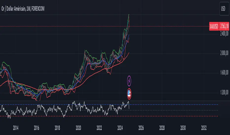
XAUUSD Trend Strategy### Description of the XAUUSD Trading Strategy with Pine Script
This strategy is designed to trade gold (**XAUUSD**) using proven technical analysis principles. It combines key indicators such as **Exponential Moving Averages (EMA)**, the **Relative Strength Index (RSI)**, and **Bollinger Bands** to identify trading opportunities in trending market conditions.
---
#### Objective:
To maximize profits by identifying trend-aligned entry points while minimizing risks through well-defined Stop Loss and Take Profit levels.
---
### How It Works
1. **Indicators Used:**
- **Exponential Moving Averages (EMA):** Tracks short-term and long-term trends to confirm market direction.
- **Relative Strength Index (RSI):** Detects overbought or oversold conditions for potential reversals or trend continuation.
- **Bollinger Bands:** Measures volatility to identify breakout or reversion points.
2. **Entry Rules:**
- **Long (Buy):** Triggered when:
- The short-term EMA crosses above the long-term EMA (bullish trend confirmation).
- RSI exits oversold territory (<30), signaling buying momentum.
- The price breaks above the upper Bollinger Band, indicating a strong trend.
- **Short (Sell):** Triggered when:
- The short-term EMA crosses below the long-term EMA (bearish trend confirmation).
- RSI exits overbought territory (>70), signaling selling momentum.
- The price breaks below the lower Bollinger Band, indicating a strong downtrend.
3. **Risk Management:**
- **Stop Loss:** Automatically calculated based on a percentage of equity risk (customizable via inputs).
- **Take Profit:** Defined using a risk-to-reward ratio, ensuring consistent profitability when trades succeed.
4. **Visualization:**
- The chart displays the EMAs, Bollinger Bands, and entry/exit points for clear analysis.
---
### Key Features:
- **Customizable Parameters:** You can adjust EMAs, RSI thresholds, Bollinger Band settings, and risk levels to suit your trading style.
- **Alerts:** Automatic alerts for potential trade setups.
- **Backtesting-Ready:** Easily test historical performance on TradingView.
---
This strategy is ideal for gold traders looking for a systematic, rule-based approach to trading trends with minimal emotional interference.
Pesquisar nos scripts por "profit"
Multi Fibonacci Supertrend with Signals【FIbonacciFlux】Multi Fibonacci Supertrend with Signals (MFSS)
Overview
The Multi Fibonacci Supertrend with Signals (MFSS) is an advanced technical analysis tool that combines multiple Supertrend indicators using Fibonacci ratios to identify trend directions and potential trading opportunities.
Key Features
1. Fibonacci-Based Supertrend Levels
* Factor 1 (Weak) : 0.618 - The golden ratio
* Factor 2 (Medium) : 1.618 - The Fibonacci ratio
* Factor 3 (Strong) : 2.618 - The extension ratio
2. Visual Components
* Multi-layered Trend Lines
* Different line weights for easy identification
* Progressive transparency from Factor 1 to Factor 3
* Color-coded trend directions (Green for bullish, Red for bearish)
* Dynamic Fill Areas
* Gradient fills between price and trend lines
* Visual representation of trend strength
* Automatic color adjustment based on trend direction
* Signal Indicators
* Clear BUY/SELL labels on chart
* Position-adaptive signal placement
* High-visibility color scheme
3. Signal Generation Logic
The system generates signals based on two key conditions:
* Primary Condition :
* BUY : Price crossunder Supertrend2 (Factor 1.618)
* SELL : Price crossover Supertrend2 (Factor 1.618)
* Confirmation Filter :
* Signals only trigger when Supertrend3 confirms the trend direction
* Reduces false signals in volatile markets
Technical Details
Input Parameters
* ATR Period : 10 (default)
* Customizable for different market conditions
* Affects sensitivity of all Supertrend levels
* Factor Settings :
* All factors are customizable
* Default values based on Fibonacci sequence
* Minimum value: 0.01
* Step size: 0.01
Alert System
* Built-in alert conditions
* Customizable alert messages
* Real-time notification support
Use Cases
* Trend Trading
* Identify strong trend directions
* Filter out weak signals
* Confirm trend continuations
* Risk Management
* Multiple trend levels for stop-loss placement
* Clear entry and exit signals
* Trend strength visualization
* Market Analysis
* Multi-timeframe analysis capability
* Trend strength assessment
* Market structure identification
Benefits
* Reliability
* Based on proven Supertrend algorithm
* Enhanced with Fibonacci mathematics
* Multiple confirmation levels
* Clarity
* Clear visual signals
* Easy-to-interpret interface
* Reduced noise in signal generation
* Flexibility
* Customizable parameters
* Adaptable to different markets
* Suitable for various trading styles
Performance Considerations
* Optimized code structure
* Efficient calculation methods
* Minimal resource usage
Installation and Usage
Setup
* Add indicator to chart
* Adjust parameters if needed
* Enable alerts as required
Best Practices
* Use with other confirmation tools
* Adjust factors based on market volatility
* Consider timeframe appropriateness
Backtesting Results and Strategy Performance
This indicator is specifically designed for pullback trading with optimized risk-reward ratios in trend-following strategies. Below are the detailed backtesting results from our proprietary strategy implementation:
BTCUSDT Performance (Binance)
* Test Period: Approximately 7 years
* Risk-Reward Ratio: 2:1
* Take Profit: 8%
* Stop Loss: 4%
Key Metrics (BTCUSDT):
* Net Profit: +2,579%
* Total Trades: 551
* Win Rate: 44.8%
* Profit Factor: 1.278
* Maximum Drawdown: 42.86%
ETHUSD Performance (Binance)
* Risk-Reward Ratio: 4.33:1
* Take Profit: 13%
* Stop Loss: 3%
Key Metrics (ETHUSD):
* Net Profit: +8,563%
* Total Trades: 581
* Win Rate: 32%
* Profit Factor: 1.32
* Maximum Drawdown: 55%
Strategy Highlights:
* Optimized for pullback trading in strong trends
* Focus on high risk-reward ratios
* Proven effectiveness in major cryptocurrency pairs
* Consistent performance across different market conditions
* Robust profit factor despite moderate win rates
Note: These results are from our proprietary strategy implementation and should be used as reference only. Individual results may vary based on market conditions and implementation.
Important Considerations:
* The strategy demonstrates strong profitability despite lower win rates, emphasizing the importance of proper risk-reward ratios
* Higher drawdowns are compensated by significant overall returns
* The system shows adaptability across different cryptocurrencies with consistent profit factors
* Results suggest optimal performance in volatile crypto markets
Real Trading Examples
BTCUSDT 4-Hour Chart Analysis
Example of pullback strategy implementation on Bitcoin, showing clear trend definition and entry points
ETHUSDT 4-Hour Chart Analysis
Ethereum chart demonstrating effective signal generation during strong trends
BTCUSDT Detailed Signal Example (15-Minute Scalping)
Close-up view of signal generation and trend confirmation process on 15-minute timeframe, demonstrating the indicator's effectiveness for scalping operations
Chart Analysis Notes:
* Green and red zones clearly indicate trend direction
* Multiple timeframe confirmation visible through different Supertrend levels
* Clear entry signals during pullbacks in established trends
* Precise stop-loss placement opportunities below support levels
Implementation Guidelines:
* Wait for main trend confirmation from Factor 3 (2.618)
* Enter trades on pullbacks to Factor 2 (1.618)
* Use Factor 1 (0.618) for fine-tuning entry points
* Place stops below the relevant Supertrend level
Footnotes:
* Charts provided are from Binance exchange, using both 4-hour and 15-minute timeframes
* Trading view screenshots captured during actual market conditions
* Indicators shown: Multi Fibonacci Supertrend with all three factors
* Time period: Recent market activity showing various market conditions
Important Notice:
These charts are for educational purposes only. Past performance does not guarantee future results. Always conduct your own analysis and risk management.
Disclaimer
This indicator is for informational purposes only. Past performance is not indicative of future results. Always conduct proper risk management and due diligence.
License
Open source under MIT License
Author's Note
Contributions and suggestions for improvement are welcome. Please feel free to fork and enhance.

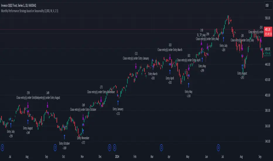
Unlock the Power of Seasonality: Monthly Performance StrategyThe Monthly Performance Strategy leverages the power of seasonality—those cyclical patterns that emerge in financial markets at specific times of the year. From tax deadlines to industry-specific events and global holidays, historical data shows that certain months can offer strong opportunities for trading. This strategy was designed to help traders capture those opportunities and take advantage of recurring market patterns through an automated and highly customizable approach.
The Inspiration Behind the Strategy:
This strategy began with the idea that market performance is often influenced by seasonal factors. Historically, certain months outperform others due to a variety of reasons, like earnings reports, holiday shopping, or fiscal year-end events. By identifying these periods, traders can better time their market entries and exits, giving them an advantage over those who solely rely on technical indicators or news events.
The Monthly Performance Strategy was built to take this concept and automate it. Instead of manually analyzing market data for each month, this strategy enables you to select which months you want to focus on and then executes trades based on predefined rules, saving you time and optimizing the performance of your trades.
Key Features:
Customizable Month Selection: The strategy allows traders to choose specific months to test or trade on. You can select any combination of months—for example, January, July, and December—to focus on based on historical trends. Whether you’re targeting the historically strong months like December (often driven by the 'Santa Rally') or analyzing quieter months for low volatility trades, this strategy gives you full control.
Automated Monthly Entries and Exits: The strategy automatically enters a long position on the first day of your selected month(s) and exits the trade at the beginning of the next month. This makes it perfect for traders who want to benefit from seasonal patterns without manually monitoring the market. It ensures precision in entering and exiting trades based on pre-set timeframes.
Re-entry on Stop Loss or Take Profit: One of the standout features of this strategy is its ability to re-enter a trade if a position hits the stop loss (SL) or take profit (TP) level during the selected month. If your trade reaches either a SL or TP before the month ends, the strategy will automatically re-enter a new trade the next trading day. This feature ensures that you capture multiple trading opportunities within the same month, instead of exiting entirely after a successful or unsuccessful trade. Essentially, it keeps your capital working for you throughout the entire month, not just when conditions align perfectly at the beginning.
Built-in Risk Management: Risk management is a vital part of this strategy. It incorporates an Average True Range (ATR)-based stop loss and take profit system. The ATR helps set dynamic levels based on the market’s volatility, ensuring that your stops and targets adjust to changing market conditions. This not only helps limit potential losses but also maximizes profit potential by adapting to market behavior.
Historical Performance Testing: You can backtest this strategy on any period by setting the start year. This allows traders to analyze past market data and optimize their strategy based on historical performance. You can fine-tune which months to trade based on years of data, helping you identify trends and patterns that provide the best trading results.
Versatility Across Asset Classes: While this strategy can be particularly effective for stock market indices and sector rotation, it’s versatile enough to apply to other asset classes like forex, commodities, and even cryptocurrencies. Each asset class may exhibit different seasonal behaviors, allowing you to explore opportunities across various markets with this strategy.
How It Works:
The trader selects which months to test or trade, for example, January, April, and October.
The strategy will automatically open a long position on the first trading day of each selected month.
If the trade hits either the take profit or stop loss within the month, the strategy will close the current position and re-enter a new trade on the next trading day, provided the month has not yet ended. This ensures that the strategy continues to capture any potential gains throughout the month, rather than stopping after one successful trade.
At the start of the next month, the position is closed, and if the next month is also selected, a new trade is initiated following the same process.
Risk Management and Dynamic Adjustments:
Incorporating risk management with this strategy is as easy as turning on the ATR-based system. The strategy will automatically calculate stop loss and take profit levels based on the market’s current volatility, adjusting dynamically to the conditions. This ensures that the risk is controlled while allowing for flexibility in capturing profits during both high and low volatility periods.
Maximizing the Seasonal Edge:
By automating entries and exits based on specific months and combining that with dynamic risk management, the Ultimate Monthly Performance Strategy takes advantage of seasonal patterns without requiring constant monitoring. The added re-entry feature after hitting a stop loss or take profit ensures that you are always in the game, maximizing your chances to capture profitable trades during favorable seasonal periods.
Who Can Benefit from This Strategy?
This strategy is perfect for traders who:
Want to exploit the predictable, recurring patterns that occur during specific months of the year.
Prefer a hands-off, automated trading approach that allows them to focus on other aspects of their portfolio or life.
Seek to manage risk effectively with ATR-based stop losses and take profits that adjust to market conditions.
Appreciate the ability to re-enter trades when a take profit or stop loss is hit within the month, ensuring that they don't miss out on multiple opportunities during a favorable period.
In summary, the Ultimate Monthly Performance Strategy provides traders with a comprehensive tool to capitalize on seasonal trends, optimize their trading opportunities throughout the year, and manage risk effectively. The built-in re-entry system ensures you continue to benefit from the market even after hitting targets within the same month, making it a robust strategy for traders looking to maximize their edge in any market.
Risk Disclaimer:
Trading financial markets involves significant risk and may not be suitable for all investors. The Monthly Performance Strategy is designed to help traders identify seasonal trends, but past performance does not guarantee future results. It is important to carefully consider your risk tolerance, financial situation, and trading goals before using any strategy. Always use appropriate risk management and consult with a professional financial advisor if necessary. The use of this strategy does not eliminate the risk of losses, and traders should be prepared for the possibility of losing their entire investment. Be sure to test the strategy on a demo account before applying it in live markets.
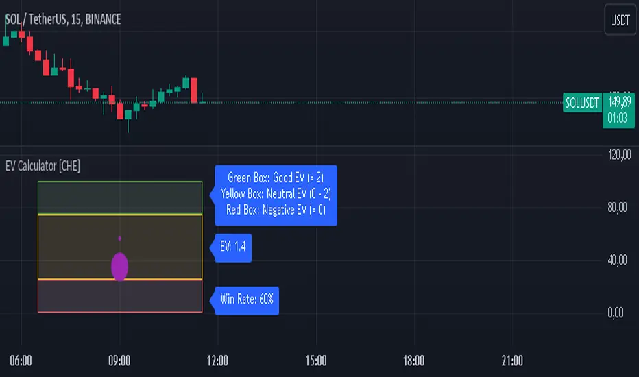
EV Calculator [CHE]EV Calculator with Adjustable Boxes and Custom Colors for TradingView
Introduction:
As a trader, one of the key metrics you need to evaluate is the Expected Value (EV) of your trading strategy. Understanding EV helps you gauge whether your trades will be profitable in the long run. This TradingView script allows you to visualize your EV alongside customizable win rates and risk-to-reward ratios. With adjustable visual components, you can quickly determine whether your trading strategy has a positive or negative EV, and make informed decisions.
Features of the Script:
1. Customizable Inputs:
- Win Rate: Set your win probability (0.0 to 1.0), which represents how often your strategy is successful.
- Risk and Reward: Define how much you're risking and the potential reward for each trade.
2. Visual Representation:
- The script creates colored boxes representing different EV scenarios:
- Green Box: Indicates a good EV (>2), suggesting a highly profitable strategy.
- Yellow Box: Represents a neutral EV (between 0 and 2), where the strategy could work but is not optimal.
- Red Box: Shows a negative EV (<0), signaling that the strategy may lead to losses.
3. Adjustable Box Size:
- You can modify the width and height of the boxes to fit your chart display preferences, giving you better visual clarity based on your screen or chart style.
4. Dynamic Labels:
- Each bar in the chart includes dynamic labels showing:
- Win Rate: Displays the percentage chance of success.
- EV Value: Shows the calculated expected value based on the win rate and risk-reward ratio.
- Guide: Explains what each colored box means so that you can easily interpret the chart.
5. Scalability and Flexibility:
- The script only keeps a maximum of 20 recent entries, ensuring that your chart stays clean and organized.
- Both the number of labels and boxes adjust automatically to match your preferred settings, enhancing usability.
How the EV Calculation Works:
The formula for EV is based on a standard risk-to-reward model:
EV = (Win\ Rate \times Reward) - (Loss\ Probability \times Risk)
For example:
- If your win rate is 60% and your risk-to-reward ratio is 1:3, the script will calculate whether this strategy is expected to yield positive returns or result in long-term losses.
Example Use Case:
Let's say you are trading with a 60% win rate, risking 1 unit to gain 3 units. The script calculates that your EV is positive and represents this with a Green Box, showing you that your strategy has a high likelihood of being profitable. If your strategy slips and the win rate drops, the EV calculation will adjust, and you may see Yellow or Red Boxes, signaling a need for adjustment.
Final Thoughts:
This script is designed for traders who want to take their analysis beyond the basics. By providing real-time visualization of your EV, you can better assess whether your strategy is sound and make adjustments as needed.
How to Use:
- Adjust the input parameters for Win Rate, Risk, and Reward to match your trading strategy.
- Observe the colored boxes and labels to quickly understand if your current strategy is in a healthy EV zone.
- Use this visual feedback to refine your approach and stay on track towards profitability.
This tool simplifies the complex calculations behind EV and turns it into an intuitive and powerful decision-making aid for traders.
Now you're ready to integrate the EV Calculator with Adjustable Boxes and Custom Colors into your trading routine and start optimizing your strategies for long-term success!
Happy Trading and best regards Chervolino
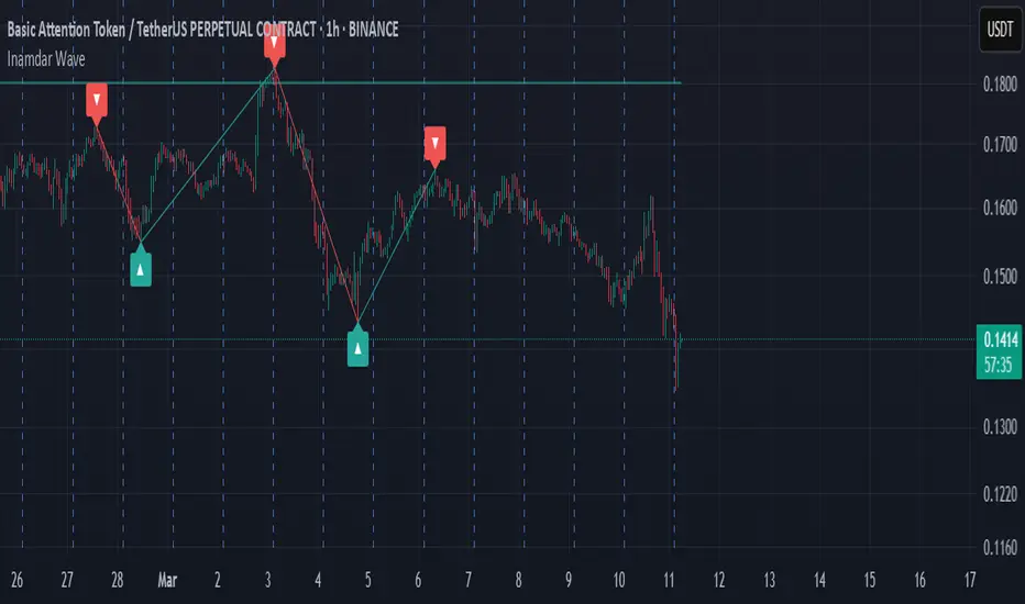
Inamdar Wave - Winning Wave
The **"Inamdar Wave"**, also known as the **"Winning Wave"**, is a cutting-edge market indicator designed to help traders ride the waves of momentum and capitalize on high-probability opportunities. With its unique ability to adapt to market shifts, the Inamdar Wave ensures you're always in sync with the market's most profitable moves, making it an indispensable tool for traders looking for consistent success.
### Key Features of the "Inamdar Wave":
1. **Dynamic Market Movement Detection**:
- The **Inamdar Wave** tracks the market’s momentum and identifies clear waves of movement, allowing traders to catch both upswings and downswings with ease.
- This indicator dynamically adjusts based on price action and volatility, ensuring you're always aligned with the market’s natural flow.
- Whether the market is trending or ranging, the **Inamdar Wave** keeps you on the right path, helping you surf the market's waves effortlessly.
2. **Highly Profitable Buy/Sell Signals**:
- The **Inamdar Wave** generates precise buy and sell signals that guide you to the most profitable entry and exit points.
- Its built-in filters ensure you avoid market noise, focusing only on high-probability trades that maximize your potential for profit.
- You’ll confidently enter trades at the start of each new wave, ensuring you ride the momentum for maximum gains.
3. **Visual Wave Highlighting**:
- Color-coded zones help you easily spot bullish (upward) and bearish (downward) waves.
- Green highlights signal upward waves, while red zones indicate downward waves, making it visually simple to recognize the current market direction.
- This feature allows for quick decision-making and a clear understanding of the market's direction at a glance.
4. **Tailored for Any Market Condition**:
- Whether you’re trading a calm or highly volatile market, the **Inamdar Wave** adapts to the changing conditions, ensuring consistent performance across all environments.
- Its flexibility allows it to work seamlessly with any asset class—stocks, forex, crypto, or commodities—making it an all-in-one solution for traders.
- The **Inamdar Wave**'s real-time adjustments keep it relevant regardless of market conditions or timeframes.
5. **Real-Time Alerts**:
- Get instant alerts when a new wave begins, whether it's a buy, sell, or wave reversal.
- You’ll never miss out on a profitable opportunity with real-time notifications that keep you one step ahead of the market.
- These alerts help you act quickly, maximizing the potential of every market movement.
### Inputs:
- **Wave Period**: Customize the sensitivity of the wave detection with adjustable periods to suit your trading style.
- **Signal Source**: Choose from different price sources to fine-tune how the **Inamdar Wave** reacts to market movements.
- **Signal Strength**: Control the sensitivity of wave detection to focus on only the strongest and most profitable moves.
- **Buy/Sell Signals**: Easily toggle buy/sell signals on your chart for enhanced clarity.
- **Wave Highlighting**: Turn visual wave highlights on or off, depending on your preference.
### Use Case:
The **Inamdar Wave** is perfect for traders looking to capture the most profitable waves in any market. Whether you're a short-term scalper or a long-term trend follower, this indicator keeps you in sync with the market’s natural rhythm, ensuring that you're always riding the winning wave. With its powerful buy/sell signals and dynamic wave detection, you'll be better positioned to take advantage of market momentum and secure consistent profits.
In conclusion, the **"Inamdar Wave"** is not just another indicator—it’s your key to riding the market’s most profitable waves with precision and confidence. By following the signals and staying in tune with the market’s natural flow, you’ll be able to maximize your gains and minimize your risks, ensuring a successful trading journey.
Optimized Heikin Ashi Strategy with Buy/Sell OptionsStrategy Name:
Optimized Heikin Ashi Strategy with Buy/Sell Options
Description:
The Optimized Heikin Ashi Strategy is a trend-following strategy designed to capitalize on market trends by utilizing the smoothness of Heikin Ashi candles. This strategy provides flexible options for trading, allowing users to choose between Buy Only (long-only), Sell Only (short-only), or using both in alternating conditions based on the Heikin Ashi candle signals. The strategy works on any market, but it performs especially well in markets where trends are prevalent, such as cryptocurrency or Forex.
This script offers customizable parameters for the backtest period, Heikin Ashi timeframe, stop loss, and take profit levels, allowing traders to optimize the strategy for their preferred markets or assets.
Key Features:
Trade Type Options:
Buy Only: Enter a long position when a green Heikin Ashi candle appears and exit when a red candle appears.
Sell Only: Enter a short position when a red Heikin Ashi candle appears and exit when a green candle appears.
Stop Loss and Take Profit:
Customizable stop loss and take profit percentages allow for flexible risk management.
The default stop loss is set to 2%, and the default take profit is set to 4%, maintaining a favorable risk/reward ratio.
Heikin Ashi Timeframe:
Traders can select the desired timeframe for Heikin Ashi candle calculation (e.g., 4-hour Heikin Ashi candles for a 1-hour chart).
The strategy smooths out price action and reduces noise, providing clearer signals for entry and exit.
Inputs:
Backtest Start Date / End Date: Specify the period for testing the strategy’s performance.
Heikin Ashi Timeframe: Select the timeframe for Heikin Ashi candle generation. A higher timeframe helps smooth the trend, which is beneficial for trading lower timeframes.
Stop Loss (in %) and Take Profit (in %): Enable or disable stop loss and take profit, and adjust the levels based on market conditions.
Trade Type: Choose between Buy Only or Sell Only based on your market outlook and strategy preference.
Strategy Performance:
In testing with BTC/USD, this strategy performed well in a 4-hour Heikin Ashi timeframe applied on a 1-hour chart over a period from January 1, 2024, to September 12, 2024. The results were as follows:
Initial Capital: 1 USD
Order Size: 100% of equity
Net Profit: +30.74 USD (3,073.52% return)
Percent Profitable: 78.28% of trades were winners.
Profit Factor: 15.825, indicating that the strategy's profitable trades far outweighed its losses.
Max Drawdown: 4.21%, showing low risk exposure relative to the large profit potential.
This strategy is ideal for both beginner and advanced traders who are looking to follow trends and avoid market noise by using Heikin Ashi candles. It is also well-suited for traders who prefer automated risk management through the use of stop loss and take profit levels.
Recommended Use:
Best Markets: This strategy works well on trending markets like cryptocurrency, Forex, or indices.
Timeframes: Works best when applied to lower timeframes (e.g., 1-hour chart) with a higher Heikin Ashi timeframe (e.g., 4-hour candles) to smooth out price action.
Leverage: The strategy performs well with leverage, but users should consider using 2x to 3x leverage to avoid excessive risk and potential liquidation. The strategy's low drawdown allows for moderate leverage use while maintaining risk control.
Customization: Traders can adjust the stop loss and take profit percentages based on their risk appetite and market conditions. A default setting of a 2% stop loss and 4% take profit provides a balanced risk/reward ratio.
Notes:
Risk Management: Traders should enable stop loss and take profit settings to maintain effective risk management and prevent large drawdowns during volatile market conditions.
Optimization: This strategy can be further optimized by adjusting the Heikin Ashi timeframe and risk parameters based on specific market conditions and assets.
Backtesting: The built-in backtesting functionality allows traders to test the strategy across different market conditions and historical data to ensure robustness before applying it to live trading.
How to Apply:
Select your preferred market and chart.
Choose the appropriate Heikin Ashi timeframe based on the chart's timeframe. (e.g., use 4-hour Heikin Ashi candles for 1-hour chart trends).
Adjust stop loss and take profit based on your risk management preference.
Run backtesting to evaluate its performance before applying it in live trading.
This strategy can be further modified and optimized based on personal trading style and market conditions. It’s important to monitor performance regularly and adjust settings as needed to align with market behavior.

Intramarket Difference Index StrategyHi Traders !!
The IDI Strategy:
In layman’s terms this strategy compares two indicators across markets and exploits their differences.
note: it is best the two markets are correlated as then we know we are trading a short to long term deviation from both markets' general trend with the assumption both markets will trend again sometime in the future thereby exhausting our trading opportunity.
📍 Import Notes:
This Strategy calculates trade position size independently (i.e. risk per trade is controlled in the user inputs tab), this means that the ‘Order size’ input in the ‘Properties’ tab will have no effect on the strategy. Why ? because this allows us to define custom position size algorithms which we can use to improve our risk management and equity growth over time. Here we have the option to have fixed quantity or fixed percentage of equity ATR (Average True Range) based stops in addition to the turtle trading position size algorithm.
‘Pyramiding’ does not work for this strategy’, similar to the order size input togeling this input will have no effect on the strategy as the strategy explicitly defines the maximum order size to be 1.
This strategy is not perfect, and as of writing of this post I have not traded this algo.
Always take your time to backtests and debug the strategy.
🔷 The IDI Strategy:
By default this strategy pulls data from your current TV chart and then compares it to the base market, be default BINANCE:BTCUSD . The strategy pulls SMA and RSI data from either market (we call this the difference data), standardizes the data (solving the different unit problem across markets) such that it is comparable and then differentiates the data, calling the result of this transformation and difference the Intramarket Difference (ID). The formula for the the ID is
ID = market1_diff_data - market2_diff_data (1)
Where
market(i)_diff_data = diff_data / ATR(j)_market(i)^0.5,
where i = {1, 2} and j = the natural numbers excluding 0
Formula (1) interpretation is the following
When ID > 0: this means the current market outperforms the base market
When ID = 0: Markets are at long run equilibrium
When ID < 0: this means the current market underperforms the base market
To form the strategy we define one of two strategy type’s which are Trend and Mean Revesion respectively.
🔸 Trend Case:
Given the ‘‘Strategy Type’’ is equal to TREND we define a threshold for which if the ID crosses over we go long and if the ID crosses under the negative of the threshold we go short.
The motivating idea is that the ID is an indicator of the two symbols being out of sync, and given we know volatility clustering, momentum and mean reversion of anomalies to be a stylised fact of financial data we can construct a trading premise. Let's first talk more about this premise.
For some markets (cryptocurrency markets - synthetic symbols in TV) the stylised fact of momentum is true, this means that higher momentum is followed by higher momentum, and given we know momentum to be a vector quantity (with magnitude and direction) this momentum can be both positive and negative i.e. when the ID crosses above some threshold we make an assumption it will continue in that direction for some time before executing back to its long run equilibrium of 0 which is a reasonable assumption to make if the market are correlated. For example for the BTCUSD - ETHUSD pair, if the ID > +threshold (inputs for MA and RSI based ID thresholds are found under the ‘‘INTRAMARKET DIFFERENCE INDEX’’ group’), ETHUSD outperforms BTCUSD, we assume the momentum to continue so we go long ETHUSD.
In the standard case we would exit the market when the IDI returns to its long run equilibrium of 0 (for the positive case the ID may return to 0 because ETH’s difference data may have decreased or BTC’s difference data may have increased). However in this strategy we will not define this as our exit condition, why ?
This is because we want to ‘‘let our winners run’’, to achieve this we define a trailing Donchian Channel stop loss (along with a fixed ATR based stop as our volatility proxy). If we were too use the 0 exit the strategy may print a buy signal (ID > +threshold in the simple case, market regimes may be used), return to 0 and then print another buy signal, and this process can loop may times, this high trade frequency means we fail capture the entire market move lowering our profit, furthermore on lower time frames this high trade frequencies mean we pay more transaction costs (due to price slippage, commission and big-ask spread) which means less profit.
By capturing the sum of many momentum moves we are essentially following the trend hence the trend following strategy type.
Here we also print the IDI (with default strategy settings with the MA difference type), we can see that by letting our winners run we may catch many valid momentum moves, that results in a larger final pnl that if we would otherwise exit based on the equilibrium condition(Valid trades are denoted by solid green and red arrows respectively and all other valid trades which occur within the original signal are light green and red small arrows).
another example...
Note: if you would like to plot the IDI separately copy and paste the following code in a new Pine Script indicator template.
indicator("IDI")
// INTRAMARKET INDEX
var string g_idi = "intramarket diffirence index"
ui_index_1 = input.symbol("BINANCE:BTCUSD", title = "Base market", group = g_idi)
// ui_index_2 = input.symbol("BINANCE:ETHUSD", title = "Quote Market", group = g_idi)
type = input.string("MA", title = "Differrencing Series", options = , group = g_idi)
ui_ma_lkb = input.int(24, title = "lookback of ma and volatility scaling constant", group = g_idi)
ui_rsi_lkb = input.int(14, title = "Lookback of RSI", group = g_idi)
ui_atr_lkb = input.int(300, title = "ATR lookback - Normalising value", group = g_idi)
ui_ma_threshold = input.float(5, title = "Threshold of Upward/Downward Trend (MA)", group = g_idi)
ui_rsi_threshold = input.float(20, title = "Threshold of Upward/Downward Trend (RSI)", group = g_idi)
//>>+----------------------------------------------------------------+}
// CUSTOM FUNCTIONS |
//<<+----------------------------------------------------------------+{
// construct UDT (User defined type) containing the IDI (Intramarket Difference Index) source values
// UDT will hold many variables / functions grouped under the UDT
type functions
float Close // close price
float ma // ma of symbol
float rsi // rsi of the asset
float atr // atr of the asset
// the security data
getUDTdata(symbol, malookback, rsilookback, atrlookback) =>
indexHighTF = barstate.isrealtime ? 1 : 0
= request.security(symbol, timeframe = timeframe.period,
expression = [close , // Instentiate UDT variables
ta.sma(close, malookback) ,
ta.rsi(close, rsilookback) ,
ta.atr(atrlookback) ])
data = functions.new(close_, ma_, rsi_, atr_)
data
// Intramerket Difference Index
idi(type, symbol1, malookback, rsilookback, atrlookback, mathreshold, rsithreshold) =>
threshold = float(na)
index1 = getUDTdata(symbol1, malookback, rsilookback, atrlookback)
index2 = getUDTdata(syminfo.tickerid, malookback, rsilookback, atrlookback)
// declare difference variables for both base and quote symbols, conditional on which difference type is selected
var diffindex1 = 0.0, var diffindex2 = 0.0,
// declare Intramarket Difference Index based on series type, note
// if > 0, index 2 outpreforms index 1, buy index 2 (momentum based) until equalibrium
// if < 0, index 2 underpreforms index 1, sell index 1 (momentum based) until equalibrium
// for idi to be valid both series must be stationary and normalised so both series hae he same scale
intramarket_difference = 0.0
if type == "MA"
threshold := mathreshold
diffindex1 := (index1.Close - index1.ma) / math.pow(index1.atr*malookback, 0.5)
diffindex2 := (index2.Close - index2.ma) / math.pow(index2.atr*malookback, 0.5)
intramarket_difference := diffindex2 - diffindex1
else if type == "RSI"
threshold := rsilookback
diffindex1 := index1.rsi
diffindex2 := index2.rsi
intramarket_difference := diffindex2 - diffindex1
//>>+----------------------------------------------------------------+}
// STRATEGY FUNCTIONS CALLS |
//<<+----------------------------------------------------------------+{
// plot the intramarket difference
= idi(type,
ui_index_1,
ui_ma_lkb,
ui_rsi_lkb,
ui_atr_lkb,
ui_ma_threshold,
ui_rsi_threshold)
//>>+----------------------------------------------------------------+}
plot(intramarket_difference, color = color.orange)
hline(type == "MA" ? ui_ma_threshold : ui_rsi_threshold, color = color.green)
hline(type == "MA" ? -ui_ma_threshold : -ui_rsi_threshold, color = color.red)
hline(0)
Note it is possible that after printing a buy the strategy then prints many sell signals before returning to a buy, which again has the same implication (less profit. Potentially because we exit early only for price to continue upwards hence missing the larger "trend"). The image below showcases this cenario and again, by allowing our winner to run we may capture more profit (theoretically).
This should be clear...
🔸 Mean Reversion Case:
We stated prior that mean reversion of anomalies is an standerdies fact of financial data, how can we exploit this ?
We exploit this by normalizing the ID by applying the Ehlers fisher transformation. The transformed data is then assumed to be approximately normally distributed. To form the strategy we employ the same logic as for the z score, if the FT normalized ID > 2.5 (< -2.5) we buy (short). Our exit conditions remain unchanged (fixed ATR stop and trailing Donchian Trailing stop)
🔷 Position Sizing:
If ‘‘Fixed Risk From Initial Balance’’ is toggled true this means we risk a fixed percentage of our initial balance, if false we risk a fixed percentage of our equity (current balance).
Note we also employ a volatility adjusted position sizing formula, the turtle training method which is defined as follows.
Turtle position size = (1/ r * ATR * DV) * C
Where,
r = risk factor coefficient (default is 20)
ATR(j) = risk proxy, over j times steps
DV = Dollar Volatility, where DV = (1/Asset Price) * Capital at Risk
🔷 Risk Management:
Correct money management means we can limit risk and increase reward (theoretically). Here we employ
Max loss and gain per day
Max loss per trade
Max number of consecutive losing trades until trade skip
To read more see the tooltips (info circle).
🔷 Take Profit:
By defualt the script uses a Donchain Channel as a trailing stop and take profit, In addition to this the script defines a fixed ATR stop losses (by defualt, this covers cases where the DC range may be to wide making a fixed ATR stop usefull), ATR take profits however are defined but optional.
ATR SL and TP defined for all trades
🔷 Hurst Regime (Regime Filter):
The Hurst Exponent (H) aims to segment the market into three different states, Trending (H > 0.5), Random Geometric Brownian Motion (H = 0.5) and Mean Reverting / Contrarian (H < 0.5). In my interpretation this can be used as a trend filter that eliminates market noise.
We utilize the trending and mean reverting based states, as extra conditions required for valid trades for both strategy types respectively, in the process increasing our trade entry quality.
🔷 Example model Architecture:
Here is an example of one configuration of this strategy, combining all aspects discussed in this post.
Future Updates
- Automation integration (next update)
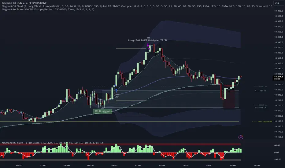
Negroni Opening Range StrategyStrategy Summary:
This tool can be used to help identify breakouts from a range during a time-zone of your choosing. It plots a pre-market range, an opening range, it also includes moving average levels that can be used as confluence, as well as plotting previous day SESSION highs and lows.
There are several options on how you wish to close out the trades, all described in more detail below.
Back-testing Inputs:
You define your timezone.
You define how many trades to open on any given day.
You decide to go: long only, short only, or long & short (CAREFUL: "Long & Short" can open trades that effectively closes-out existing ones, for better AND worse!)
You define between which times the strategy will open trades.
You define when it closes any open trades (preventing overnight trades, or leaving trades open into US data times!!).
This hopefully helps make back-testing reflect YOUR trading hours.
NOTE: Renko or Heikin-Ashi charts
For ALL strategies, don’t use Renko or Heikin-Ashi charts unless you know EXACTLY the implications.
Specific to my strategy, using a renko chart can make this 85-90% profitable (I wish it was!!) Although they can be useful, renko charts don’t always capture real wicks, so the renko chart may show your trade up-only but your broker (who is not using renko!!) will have likely stopped you out on a wick somewhere along the line.
NOTE: TradingView ‘Deep backtesting’
For ALL strategies, be cynical of all backtesting (e.g. repainting issues etc) as well as ‘Deep backtesting’ results.
Specific to this strategy, the default settings here SHOULD BE OK, but unfortunately at the time of writing, we can’t see on the chart what exactly ‘deep backtesting’ is calculating. In the past I have noted a number of trades that were not closed at the end of the day, despite my ‘end of day’ trade closing being enabled, so there were big winners and losers that would not have materialized otherwise. As I say, this seems ok at these settings but just always be cynical!!
Opening Range Inputs
You define a pre-market range (example: 08:00 - 09:00).
You define an opening range (example: 09:00 - 09:30).
The strategy will give an update at the close of the opening range to let you know if the opening range has broken out the pre-market range (OR Breakout), or if it has remained inside (OR Inside). The label appears at the end of the opening range NOT at the bar that ‘broke-out’.
This is just a visual cue for you, it has no bearing on what the strategy will do.
The strategy default will trade off the pre-market range, but you can untick this if you prefer to trade off the opening range.
Opening Trades:
Strategy goes long when the bar (CLOSE) crosses-over the ‘pre-market’ high (not the ‘opening range’ high); and the time is within your trading session, and you have not maxed out your number of trades for the day!
Strategy goes short when the bar (CLOSE) crosses-under the ‘pre-market’ low (not the ‘opening range low); and the time is within your trading session, and you have not maxed out your number of trades for the day!
Remember, you can untick this if you prefer to trade off the opening range instead.
NOTES:
Using momentum indicators can help (RSI and MACD): especially to trade range plays in failed breakouts, when momentum shifts… but the strategy won’t do this for you!
Using an anchored vwap at the session open can also provide nice confluence, as well as take-profit levels at the upper/lower of 3x standard deviation.
CLOSING TRADES:
You have 6 take-profit (TP) options:
1) Full TP: uses ATR Multiplier - Full TP at the ATR parameters as defined in inputs.
2) Take Partial profits: ATR Multiplier - Takes partial profits based on parameters as defined in inputs (i.e close 40% of original trade at TP1, close another 40% of original trade at TP2, then the remainder at Full TP as set in option 1.).
3) Full TP: Trailing Stop - Applies a Trailing Stop at the number of points, as defined in inputs.
4) Full TP: MA cross - Takes profit when price crosses ‘Trend MA’ as defined in inputs.
5) Scalp: Points - closes at a set number of points, as defined in inputs.
6) Full TP: PMKT Multiplier - places a SL at opposite pre-market Hi/Low (we go long at a break-out of the pre-market high, 50% would place a SL at the pre-market range mid-point; 100% would place a SL at the pre-market low)'. This takes profit at the input set in option 1).
Several Fundamentals in One [aep]
**Financial Ratios Indicator**
This comprehensive Financial Ratios Indicator combines various essential metrics to help traders and investors evaluate the financial health of companies at a glance. The following categories are included:
### Valuation Ratios
- **P/B Ratio (Price to Book Ratio)**: Assesses if a stock is undervalued or overvalued by comparing its market price to its book value.
- **P/E Ratio TTM (Price to Earnings Ratio Trailing Twelve Months)**: Indicates how many years of earnings would be needed to pay the current stock price by comparing the stock price to earnings per share over the last twelve months.
- **P/FCF Ratio TTM (Price to Free Cash Flow Ratio Trailing Twelve Months)**: Evaluates a company's ability to generate free cash flow by comparing the market price to free cash flow per share over the last twelve months.
- **Tobin Q Ratio**: Indicates whether the market is overvaluing or undervaluing a company’s assets by comparing market value to replacement cost.
- **Piotroski F-Score (0-9)**: A scoring system that identifies financially strong companies based on fundamental metrics.
### Efficiency
- **Net Margin % TTM**: Measures profitability by calculating the percentage of revenue that becomes net profit after all expenses and taxes.
- **Free Cashflow Margin %**: Indicates a company’s efficiency in generating free cash flow from its revenues by showing the percentage of revenue that translates into free cash flow.
- **ROE%, ROIC%, ROA%**: Evaluate a company’s efficiency in generating profits from equity, invested capital, and total assets, respectively.
### Liquidity Metrics
- **Debt to Equity Ratio**: Shows the level of debt relative to equity, helping assess financial leverage.
- **Current Ratio**: Measures a company's ability to pay short-term debts by comparing current assets to current liabilities.
- **Long Term Debt to Assets**: Evaluates the level of long-term debt in relation to total assets.
### Dividend Policy
- **Retention Ratio % TTM**: Indicates the proportion of earnings reinvested in the company instead of distributed as dividends.
- **Dividend/Earnings Ratio % TTM**: Measures the percentage of earnings paid out as dividends to shareholders.
- **RORE % TTM (Return on Retained Earnings)**: Assesses how effectively a company utilizes retained earnings to generate additional profits.
- **Dividend Yield %**: Indicates the dividend yield of a stock by comparing annual dividends per share to the current stock price.
### Growth Ratios
- **EPS 1yr Growth %**: Measures the percentage growth of earnings per share over the last year.
- **Revenue 1yr Growth %**: Evaluates the percentage growth of revenue over the last year.
- **Sustainable Growth Rate**: Indicates the growth rate a company can maintain without increasing debt, assessing sustainable growth using internal resources.
Utilize this indicator to streamline your analysis of financial performance and make informed trading decisions.

Fractal Breakout Trend Following StrategyOverview
The Fractal Breakout Trend Following Strategy is a trend-following system which utilizes the Willams Fractals and Alligator to execute the long trades on the fractal's breakouts which have a high probability to be the new uptrend phase beginning. This system also uses the normalized Average True Range indicator to filter trades after a large moves, because it's more likely to see the trend continuation after a consolidation period. Strategy can execute only long trades.
Unique Features
Trend and volatility filtering system: Strategy uses Williams Alligator to filter the counter-trend fractals breakouts and normalized Average True Range to avoid the trades after large moves, when volatility is high
Configurable Trading Periods: Users can tailor the strategy to specific market windows, adapting to different market conditions.
Flexible Risk Management: Users can choose the stop-loss percent (by default = 3%) for trades, but strategy also has the dynamic stop-loss level using down fractals.
Methodology
The strategy places stop order at the last valid fractal breakout level. Validity of this fractal is defined by the Williams Alligator indicator. If at the moment of time when price breaking the last fractal price is higher than Alligator's teeth line (8 period SMA shifted 5 bars in the future) this is a valid breakout. Moreover strategy has the additional volatility filtering system using normalized ATR. It calculates the average normalized ATR for last user-defined number of bars and if this value lower than the user-defined threshold value the long trade is executed.
When trade is opened, script places the stop loss at the price higher of two levels: user defined stop-loss from the position entry price or down fractal validation level. The down fractal is valid with the rule, opposite as the up fractal validation. Price shall break to the downside the last down fractal below the Willians Alligator's teeth line.
Strategy has no fixed take profit. Exit level changes with the down fractal validation level. If price is in strong uptrend trade is going to be active until last down fractal is not valid. Strategy closes trade when price hits the down fractal validation level.
Risk Management
The strategy employs a combined approach to risk management:
It allows positions to ride the trend as long as the price continues to move favorably, aiming to capture significant price movements. It features a user-defined stop-loss parameter to mitigate risks based on individual risk tolerance. By default, this stop-loss is set to a 3% drop from the entry point, but it can be adjusted according to the trader's preferences.
Justification of Methodology
This strategy leverages Williams Fractals to open long trade when price has broken the key resistance level to the upside. This resistance level is the last up fractal and is shall be broken above the Williams Alligator's teeth line to be qualified as the valid breakout according to this strategy. The Alligator filtering increases the probability to avoid the false breakouts against the current trend.
Moreover strategy has an additional filter using Average True Range(ATR) indicator. If average value of ATR for the last user-defined number of bars is lower than user-defined threshold strategy can open the long trade according to open trade condition above. The logic here is following: we want to open trades after period of price consolidation inside the range because before and after a big move price is more likely to be in sideways, but we need a trend move to have a profit.
Another one important feature is how the exit condition is defined. On the one hand, strategy has the user-defined stop-loss (3% below the entry price by default). It's made to give users the opportunity to restrict their losses according to their risk-tolerance. On the other hand, strategy utilizes the dynamic exit level which is defined by down fractal activation. If we assume the breaking up fractal is the beginning of the uptrend, breaking down fractal can be the start of downtrend phase. We don't want to be in long trade if there is a high probability of reversal to the downside. This approach helps to not keep open trade if trend is not developing and hold it if price continues going up.
Backtest Results
Operating window: Date range of backtests is 2023.01.01 - 2024.05.01. It is chosen to let the strategy to close all opened positions.
Commission and Slippage: Includes a standard Binance commission of 0.1% and accounts for possible slippage over 5 ticks.
Initial capital: 10000 USDT
Percent of capital used in every trade: 30%
Maximum Single Position Loss: -3.19%
Maximum Single Profit: +24.97%
Net Profit: +3036.90 USDT (+30.37%)
Total Trades: 83 (28.92% win rate)
Profit Factor: 1.953
Maximum Accumulated Loss: 963.98 USDT (-8.29%)
Average Profit per Trade: 36.59 USDT (+1.12%)
Average Trade Duration: 72 hours
These results are obtained with realistic parameters representing trading conditions observed at major exchanges such as Binance and with realistic trading portfolio usage parameters.
How to Use
Add the script to favorites for easy access.
Apply to the desired timeframe and chart (optimal performance observed on 4h and higher time frames and the BTC/USDT).
Configure settings using the dropdown choice list in the built-in menu.
Set up alerts to automate strategy positions through web hook with the text: {{strategy.order.alert_message}}
Disclaimer:
Educational and informational tool reflecting Skyrex commitment to informed trading. Past performance does not guarantee future results. Test strategies in a simulated environment before live implementation

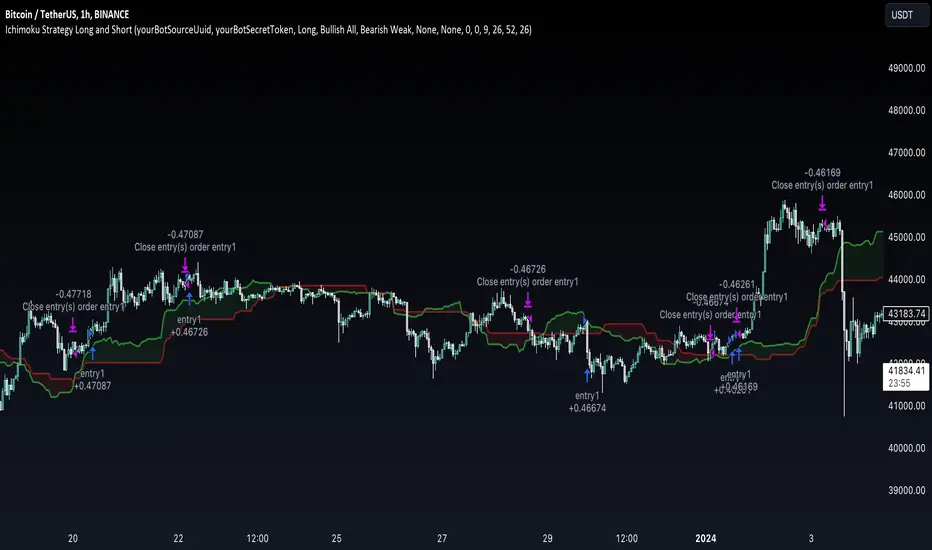
Ichimoku Clouds Strategy Long and ShortOverview:
The Ichimoku Clouds Strategy leverages the Ichimoku Kinko Hyo technique to offer traders a range of innovative features, enhancing market analysis and trading efficiency. This strategy is distinct in its combination of standard methodology and advanced customization, making it suitable for both novice and experienced traders.
Unique Features:
Enhanced Interpretation: The strategy introduces weak, neutral, and strong bullish/bearish signals, enabling detailed interpretation of the Ichimoku cloud and direct chart plotting.
Configurable Trading Periods: Users can tailor the strategy to specific market windows, adapting to different market conditions.
Dual Trading Modes: Long and Short modes are available, allowing alignment with market trends.
Flexible Risk Management: Offers three styles in each mode, combining fixed risk management with dynamic indicator states for versatile trade management.
Indicator Line Plotting: Enables plotting of Ichimoku indicator lines on the chart for visual decision-making support.
Methodology:
The strategy utilizes the standard Ichimoku Kinko Hyo model, interpreting indicator values with settings adjustable through a user-friendly menu. This approach is enhanced by TradingView's built-in strategy tester for customization and market selection.
Risk Management:
Our approach to risk management is dynamic and indicator-centric. With data from the last year, we focus on dynamic indicator states interpretations to mitigate manual setting causing human factor biases. Users still have the option to set a fixed stop loss and/or take profit per position using the corresponding parameters in settings, aligning with their risk tolerance.
Backtest Results:
Operating window: Date range of backtests is 2023.01.01 - 2024.01.04. It is chosen to let the strategy to close all opened positions.
Commission and Slippage: Includes a standard Binance commission of 0.1% and accounts for possible slippage over 5 ticks.
Maximum Single Position Loss: -6.29%
Maximum Single Profit: 22.32%
Net Profit: +10 901.95 USDT (+109.02%)
Total Trades: 119 (51.26% profitability)
Profit Factor: 1.775
Maximum Accumulated Loss: 4 185.37 USDT (-22.87%)
Average Profit per Trade: 91.67 USDT (+0.7%)
Average Trade Duration: 56 hours
These results are obtained with realistic parameters representing trading conditions observed at major exchanges such as Binance and with realistic trading portfolio usage parameters. Backtest is calculated using deep backtest option in TradingView built-in strategy tester
How to Use:
Add the script to favorites for easy access.
Apply to the desired chart and timeframe (optimal performance observed on the 1H chart, ForEx or cryptocurrency top-10 coins with quote asset USDT).
Configure settings using the dropdown choice list in the built-in menu.
Set up alerts to automate strategy positions through web hook with the text: {{strategy.order.alert_message}}
Disclaimer:
Educational and informational tool reflecting Skyrex commitment to informed trading. Past performance does not guarantee future results. Test strategies in a simulated environment before live implementation
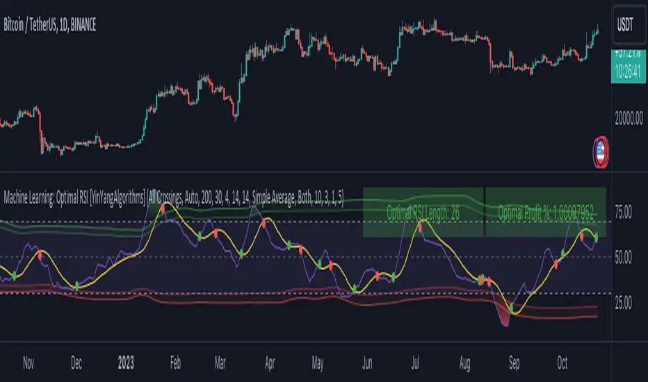
Machine Learning: Optimal RSI [YinYangAlgorithms]This Indicator, will rate multiple different lengths of RSIs to determine which RSI to RSI MA cross produced the highest profit within the lookback span. This ‘Optimal RSI’ is then passed back, and if toggled will then be thrown into a Machine Learning calculation. You have the option to Filter RSI and RSI MA’s within the Machine Learning calculation. What this does is, only other Optimal RSI’s which are in the same bullish or bearish direction (is the RSI above or below the RSI MA) will be added to the calculation.
You can either (by default) use a Simple Average; which is essentially just a Mean of all the Optimal RSI’s with a length of Machine Learning. Or, you can opt to use a k-Nearest Neighbour (KNN) calculation which takes a Fast and Slow Speed. We essentially turn the Optimal RSI into a MA with different lengths and then compare the distance between the two within our KNN Function.
RSI may very well be one of the most used Indicators for identifying crucial Overbought and Oversold locations. Not only that but when it crosses its Moving Average (MA) line it may also indicate good locations to Buy and Sell. Many traders simply use the RSI with the standard length (14), however, does that mean this is the best length?
By using the length of the top performing RSI and then applying some Machine Learning logic to it, we hope to create what may be a more accurate, smooth, optimal, RSI.
Tutorial:
This is a pretty zoomed out Perspective of what the Indicator looks like with its default settings (except with Bollinger Bands and Signals disabled). If you look at the Tables above, you’ll notice, currently the Top Performing RSI Length is 13 with an Optimal Profit % of: 1.00054973. On its default settings, what it does is Scan X amount of RSI Lengths and checks for when the RSI and RSI MA cross each other. It then records the profitability of each cross to identify which length produced the overall highest crossing profitability. Whichever length produces the highest profit is then the RSI length that is used in the plots, until another length takes its place. This may result in what we deem to be the ‘Optimal RSI’ as it is an adaptive RSI which changes based on performance.
In our next example, we changed the ‘Optimal RSI Type’ from ‘All Crossings’ to ‘Extremity Crossings’. If you compare the last two examples to each other, you’ll notice some similarities, but overall they’re quite different. The reason why is, the Optimal RSI is calculated differently. When using ‘All Crossings’ everytime the RSI and RSI MA cross, we evaluate it for profit (short and long). However, with ‘Extremity Crossings’, we only evaluate it when the RSI crosses over the RSI MA and RSI <= 40 or RSI crosses under the RSI MA and RSI >= 60. We conclude the crossing when it crosses back on its opposite of the extremity, and that is how it finds its Optimal RSI.
The way we determine the Optimal RSI is crucial to calculating which length is currently optimal.
In this next example we have zoomed in a bit, and have the full default settings on. Now we have signals (which you can set alerts for), for when the RSI and RSI MA cross (green is bullish and red is bearish). We also have our Optimal RSI Bollinger Bands enabled here too. These bands allow you to see where there may be Support and Resistance within the RSI at levels that aren’t static; such as 30 and 70. The length the RSI Bollinger Bands use is the Optimal RSI Length, allowing it to likewise change in correlation to the Optimal RSI.
In the example above, we’ve zoomed out as far as the Optimal RSI Bollinger Bands go. You’ll notice, the Bollinger Bands may act as Support and Resistance locations within and outside of the RSI Mid zone (30-70). In the next example we will highlight these areas so they may be easier to see.
Circled above, you may see how many times the Optimal RSI faced Support and Resistance locations on the Bollinger Bands. These Bollinger Bands may give a second location for Support and Resistance. The key Support and Resistance may still be the 30/50/70, however the Bollinger Bands allows us to have a more adaptive, moving form of Support and Resistance. This helps to show where it may ‘bounce’ if it surpasses any of the static levels (30/50/70).
Due to the fact that this Indicator may take a long time to execute and it can throw errors for such, we have added a Setting called: Adjust Optimal RSI Lookback and RSI Count. This settings will automatically modify the Optimal RSI Lookback Length and the RSI Count based on the Time Frame you are on and the Bar Indexes that are within. For instance, if we switch to the 1 Hour Time Frame, it will adjust the length from 200->90 and RSI Count from 30->20. If this wasn’t adjusted, the Indicator would Timeout.
You may however, change the Setting ‘Adjust Optimal RSI Lookback and RSI Count’ to ‘Manual’ from ‘Auto’. This will give you control over the ‘Optimal RSI Lookback Length’ and ‘RSI Count’ within the Settings. Please note, it will likely take some “fine tuning” to find working settings without the Indicator timing out, but there are definitely times you can find better settings than our ‘Auto’ will create; especially on higher Time Frames. The Minimum our ‘Auto’ will create is:
Optimal RSI Lookback Length: 90
RSI Count: 20
The Maximum it will create is:
Optimal RSI Lookback Length: 200
RSI Count: 30
If there isn’t much bar index history, for instance, if you’re on the 1 Day and the pair is BTC/USDT you’ll get < 4000 Bar Indexes worth of data. For this reason it is possible to manually increase the settings to say:
Optimal RSI Lookback Length: 500
RSI Count: 50
But, please note, if you make it too high, it may also lead to inaccuracies.
We will conclude our Tutorial here, hopefully this has given you some insight as to how calculating our Optimal RSI and then using it within Machine Learning may create a more adaptive RSI.
Settings:
Optimal RSI:
Show Crossing Signals: Display signals where the RSI and RSI Cross.
Show Tables: Display Information Tables to show information like, Optimal RSI Length, Best Profit, New Optimal RSI Lookback Length and New RSI Count.
Show Bollinger Bands: Show RSI Bollinger Bands. These bands work like the TDI Indicator, except its length changes as it uses the current RSI Optimal Length.
Optimal RSI Type: This is how we calculate our Optimal RSI. Do we use all RSI and RSI MA Crossings or just when it crosses within the Extremities.
Adjust Optimal RSI Lookback and RSI Count: Auto means the script will automatically adjust the Optimal RSI Lookback Length and RSI Count based on the current Time Frame and Bar Index's on chart. This will attempt to stop the script from 'Taking too long to Execute'. Manual means you have full control of the Optimal RSI Lookback Length and RSI Count.
Optimal RSI Lookback Length: How far back are we looking to see which RSI length is optimal? Please note the more bars the lower this needs to be. For instance with BTC/USDT you can use 500 here on 1D but only 200 for 15 Minutes; otherwise it will timeout.
RSI Count: How many lengths are we checking? For instance, if our 'RSI Minimum Length' is 4 and this is 30, the valid RSI lengths we check is 4-34.
RSI Minimum Length: What is the RSI length we start our scans at? We are capped with RSI Count otherwise it will cause the Indicator to timeout, so we don't want to waste any processing power on irrelevant lengths.
RSI MA Length: What length are we using to calculate the optimal RSI cross' and likewise plot our RSI MA with?
Extremity Crossings RSI Backup Length: When there is no Optimal RSI (if using Extremity Crossings), which RSI should we use instead?
Machine Learning:
Use Rational Quadratics: Rationalizing our Close may be beneficial for usage within ML calculations.
Filter RSI and RSI MA: Should we filter the RSI's before usage in ML calculations? Essentially should we only use RSI data that are of the same type as our Optimal RSI? For instance if our Optimal RSI is Bullish (RSI > RSI MA), should we only use ML RSI's that are likewise bullish?
Machine Learning Type: Are we using a Simple ML Average, KNN Mean Average, KNN Exponential Average or None?
KNN Distance Type: We need to check if distance is within the KNN Min/Max distance, which distance checks are we using.
Machine Learning Length: How far back is our Machine Learning going to keep data for.
k-Nearest Neighbour (KNN) Length: How many k-Nearest Neighbours will we account for?
Fast ML Data Length: What is our Fast ML Length? This is used with our Slow Length to create our KNN Distance.
Slow ML Data Length: What is our Slow ML Length? This is used with our Fast Length to create our KNN Distance.
If you have any questions, comments, ideas or concerns please don't hesitate to contact us.
HAPPY TRADING!
2Mars - MA / BB / SuperTrend
The 2Mars strategy is a trading approach that aims to improve trading efficiency by incorporating several simple order opening tactics. These tactics include moving average crossovers, Bollinger Bands, and SuperTrend.
Entering a Position with the 2Mars Strategy:
Moving Average Crossover: This method considers the crossing of moving averages as a signal to enter a position.
Price Crossing Bollinger Bands: If the price crosses either the upper or lower Bollinger Band, it is seen as a signal to enter a position.
Price Crossing Moving Average: If the price crosses the moving average, it is also considered a signal to enter a position.
SuperTrend and Bars confirm:
The SuperTrend indicator is used to provide additional confirmation for entering positions and setting stop loss levels. "Bars confirm" is used only for entry to positions.
Moving Average Crossover Strategy:
A moving average crossover refers to the point on a chart where there is a crossover of the signal or fast moving average, above or below the basis or slow moving average. This strategy also uses moving averages for additional orders #3.
Basis Moving Average Length: Ratio * Multiplier
Signal Moving Average Length: Multiplier
Bollinger Bands:
Bollinger Bands consist of three bands: an upper band, a lower band, and a basis moving average. However, the 2Mars strategy incorporates multiple upper and lower levels for position entry and take profit.
Basis +/- StdDev * 0.618
Basis +/- StdDev * 1.618
Basis +/- StdDev * 2.618
Additional Orders:
Additional Order #1 and #2: closing price crosses above or below the Bollinger Bands.
Additional Order #3: closing price crosses above or below the basis or signal moving average.
Take Profit:
The strategy includes three levels for taking profits, which are based on the Bollinger Bands. Additionally, a percentage of the position can be chosen to close long or short positions.
Limit Orders:
The strategy allows for entering a position using a limit order. The calculation for the limit order involves the Average True Range (ATR) for a specific period.
For long positions: Low price - ATR * Multiplier
For short positions: High price + ATR * Multiplier
Stop Loss:
To manage risk, the strategy recommends using stop loss options. The stop loss is updated with each entry order and take-profit level 3. When using the SuperTrend Confirmation, the stop loss requires confirmation of a trend change. It allows for flexible adjustment of the stop loss when the trend changes.
There are three options for setting the stop loss:
1. ATR (Average True Range):
For long positions: Low price - ATR * Long multiplier
For short positions: High price + ATR * Short multiplier
2. SuperTrend + ATR:
For long positions: SuperTrend - ATR * Long multiplier
For short positions: SuperTrend + ATR * Short multiplier
3. StdDev:
For long positions: StdDev - ATR * Long multiplier
For short positions: StdDev + ATR * Short multiplier
Flexible Stop Loss:
There is also a flexible stop loss option for the ATR and StdDev methods. It is triggered when the SuperTrend or moving average trend changes unfavorably.
For long positions: Stop-loss price + (ATR * Long multiplier) * Multiplier
For short positions: Stop-loss price - (ATR * Short multiplier) * Multiplier
How configure:
Disable SuperTrend, take profit, stop loss, additional orders and begin setting up a strategy.
Pick soucre data
Number of bars for confirm
Pick up the ratio of the base moving average and the signal moving average.
Set up a SuperTrend
Time for set up of the Bollinger Bands and the take profit
And finaly set up of stop loss and limit orders
All done!
For OKX exchange:

Trend Confirmation StrategyThe profitability and uniqueness of a trading strategy depend on various factors including market conditions, risk management, and the strategy's ability to capitalize on price movements. I'll describe the strategy provided and highlight its potential benefits and differences compared to other strategies:
Strategy Overview:
The provided strategy combines three technical indicators: Supertrend, MACD, and VWAP. It aims to identify potential entry and exit points by confirming trend direction and considering the proximity to the VWAP level. The strategy also incorporates stop-loss and take-profit mechanisms, as well as a trailing stop.
Unique Aspects and Potential Benefits:
Trend Confirmation: The strategy uses both Supertrend and MACD to confirm the trend direction. This dual confirmation can increase the likelihood of accurate trend identification and filter out false signals.
VWAP Confirmation: The strategy considers the proximity of the price to the VWAP level. This dynamic level can act as a support or resistance and provide additional context for entry decisions.
Adaptive Stop Loss: The strategy sets a stop-loss range, which helps provide some tolerance for minor price fluctuations. This adaptive approach considers market volatility and helps prevent premature stop-loss triggers.
Trailing Stop: The strategy incorporates a trailing stop mechanism to lock in profits as the trade moves in the desired direction. This can potentially enhance profitability during strong trends.
Partial Profit Booking: While not explicitly implemented in the provided code, you could consider booking partial profits when the MACD shows a crossover in the opposite direction. This aspect could help secure gains while still keeping exposure to potential further price movements.
Key Differences from Other Strategies:
Dual Indicator Confirmation: The combination of Supertrend and MACD for trend confirmation is a unique aspect of this strategy. It adds an extra layer of filtering to enhance the accuracy of entry signals.
Dynamic VWAP: Incorporating the VWAP level into the decision-making process adds a dynamic element to the strategy. VWAP is often used by institutional traders, and its inclusion can provide insights into the market sentiment.
Adaptive Stop Loss and Trailing: The strategy's use of an adaptive stop-loss range and a trailing stop can help manage risk and protect profits more effectively during changing market conditions.
Partial Profit Booking: The suggestion to consider partial profit booking upon MACD crossovers in the opposite direction is a practical approach to secure gains while staying in the trade.
Caution and Considerations:
Backtesting: Before deploying any strategy in real trading, it's crucial to thoroughly backtest it on historical data to understand its performance under various market conditions.
Risk Management: While the strategy has built-in risk management mechanisms, it's essential to carefully manage position sizes and overall portfolio risk.
Market Conditions: No strategy works well in all market conditions. It's important to be flexible and adjust the strategy or refrain from trading during particularly volatile or unpredictable periods.
Continuous Monitoring: Even though the strategy includes automated components, continuous monitoring of the trades and market conditions is necessary.
Adaptability: Markets can change over time. Traders need to be prepared to adapt the strategy as necessary to stay aligned with evolving market dynamics.

Tri-State SupertrendTri-State Supertrend: Buy, Sell, Range
( Credits: Based on "Pivot Point Supertrend" by LonesomeTheBlue.)
Tri-State Supertrend incorporates a range filter into a supertrend algorithm.
So in addition to the Buy and Sell states, we now also have a Range state.
This avoids the typical "whipsaw" problem: During a range, a standard supertrend algorithm will fire Buy and Sell signals in rapid succession. These signals are all false signals as they lead to losing positions when acted on.
In this case, a tri-state supertrend will go into Range mode and stay in this mode until price exits the range and a new trend begins.
I used Pivot Point Supertrend by LonesomeTheBlue as a starting point for this script because I believe LonesomeTheBlue's version is superior to the classic Supertrend algorithm.
This indicator has two additional parameters over Pivot Point Supertrend:
A flag to turn the range filter on or off
A range size threshold in percent
With that last parameter, you can define what a range is. The best value will depend on the asset you are trading.
Also, there are two new display options.
"Show (non-) trendline for ranges" - determines whether to draw the "trendline" inside of a range. Seeing as there is no trend in a range, this is usually just visual noise.
"Show suppressed signals" - allows you to see the Buy/Sell signals that were skipped by the range filter.
How to use Tri-State Supertrend in a strategy
You can use the Buy and Sell signals to enter positions as you would with a normal supertrend. Adding stop loss, trailing stop etc. is of course encouraged and very helpful. But what to do when the Range signal appears?
I currently run a strategy on LDO based on Tri-State Supertrend which appears to be profitable. (It will quite likely be open sourced at some point, but it is not released yet.)
In that strategy, I experimented with different actions being taken when the Range state is entered:
Continue: Just keep last position open during the range
Close: Close the last position when entering range
Reversal: During the range, execute the OPPOSITE of each signal (sell on "buy", buy on "sell")
In the backtest, it transpired that "Continue" was the most profitable option for this strategy.
How ranges are detected
The mechanism is pretty simple: During each Buy or Sell trend, we record price movement, specifically, the furthest move in the trend direction that was encountered (expressed as a percentage).
When a new signal is issued, the algorithm checks whether this value (for the last trend) is below the range size set by the user. If yes, we enter Range mode.
The same logic is used to exit Range mode. This check is performed on every bar in a range, so we can enter a buy or sell as early as possible.
I found that this simple logic works astonishingly well in practice.
Pros/cons of the range filter
A range filter is an incredibly useful addition to a supertrend and will most likely boost your profits.
You will see at most one false signal at the beginning of each range (because it takes a bit of time to detect the range); after that, no more false signals will appear over the range's entire duration. So this is a huge advantage.
There is essentially only one small price you have to pay:
When a range ends, the first Buy/Sell signal you get will be delayed over the regular supertrend's signal. This is, again, because the algorithm needs some time to detect that the range has ended. If you select a range size of, say, 1%, you will essentially lose 1% of profit in each range because of this delay.
In practice, it is very likely that the benefits of a range filter outweigh its cost. Ranges can last quite some time, equating to many false signals that the range filter will completely eliminate (all except for the first one, as explained above).
You have to do your own tests though :)

Slight Swing Momentum Strategy.Introduction:
The Swing Momentum Strategy is a quantitative trading strategy designed to capture mid-term opportunities in the financial markets by combining swing trading principles with momentum indicators. It utilizes a combination of technical indicators, including moving averages, crossover signals, and volume analysis, to generate buy and sell signals. The strategy aims to identify market trends and capitalize on price momentum for profit generation.
Highlights:
The strategy offers several key highlights that make it unique and potentially attractive to traders:
Swing Trading with Momentum: The strategy combines the principles of swing trading, which aim to capture short-to-medium-term price swings, with momentum indicators that help identify strong price trends and potential breakout opportunities.
Technical Indicator Optimization: The strategy utilizes a selection of optimized technical indicators, including moving averages and crossover signals, to filter out the noise and focus on high-probability trading setups. This optimization enhances the strategy's ability to identify favourable entry and exit points.
Risk Management: The strategy incorporates risk management techniques, such as position sizing based on equity and dynamic stop loss levels, to manage risk exposure and protect capital. This helps to minimize drawdowns and preserve profits.
Buy Condition:
The buy condition in the strategy is determined by a combination of factors, including A1, A2, A3, XG, and weeklySlope. Let's break it down:
A1 Condition: The A1 condition checks for specific price relationships. It verifies that the ratio of the highest price to the closing price is less than 1.03, the ratio of the opening price to the lowest price is less than 1.03, and the ratio of the highest price to the previous day's closing price is greater than 1.06. This condition looks for a specific pattern indicating potential bullish momentum.
A2 Condition: The A2 condition checks for price relationships related to the closing price. It verifies that the ratio of the closing price to the opening price is greater than 1.05 or that the ratio of the closing price to the previous day's closing price is greater than 1.05. This condition looks for signs of upward price movement and momentum.
A3 Condition: The A3 condition focuses on volume. It checks if the current volume crosses above the highest volume over the last 60 periods. This condition aims to identify increased buying interest and potentially confirms the strength of the potential upward price movement.
XG Condition: The XG condition combines the A1 and A2 conditions and checks if they are true for both the current and previous bars. It also verifies that the ratio of the closing price to the 5-period EMA crosses above the 9-period SMA of the same ratio. This condition helps identify potential buy signals when multiple factors align, indicating a strong bullish momentum and potential entry point.
Weekly Trend Factor: The weekly slope condition calculates the slope of the 50-period SMA over a weekly timeframe. It checks if the slope is positive, indicating an overall upward trend on a weekly basis. This condition provides additional confirmation that the stock is in an upward trend.
When all of these conditions align, the buy condition is triggered, indicating a favourable time to enter a long position.
Sell Condition:
The sell condition is relatively straightforward in the strategy:
Sell Signal: The sell condition simply checks if the closing price crosses below the 10-period EMA. When this condition is met, it indicates a potential reversal or weakening of the upward price momentum, and a sell signal is generated.
Backtest Outcome:
The strategy was backtested over the period from January 22nd, 1999 to May 3rd, 2023, using daily candlestick charts for the NASDAQ: NVDA. The strategy used an initial capital of 1,000,000 USD, The order quantity is defined as 10% of the equity. The strategy allows for pyramiding with 1 order, and the transaction fee is set at 0.03% per trade. Here are the key outcomes of the backtest:
Net Profit: 539,595.84 USD, representing a return of 53.96%.
Percent Profitable: 48.82%
Total Closed Trades: 127
Profit Factor: 2.331
Max Drawdown: 68,422.70 USD
Average Trade: 4,248.79 USD
Average Number of Bars in Trades: 11, indicating the average duration of the trades.
Conclusion:
In conclusion, the Swing Momentum Strategy is a quantitative trading approach that combines swing trading principles with momentum indicators to identify and capture mid term trading opportunities. The strategy has demonstrated promising results during backtesting, including a significant net profit and a favourable profit factor.

The Flash-Strategy (Momentum-RSI, EMA-crossover, ATR)The Flash-Strategy (Momentum-RSI, EMA-crossover, ATR)
Are you tired of manually analyzing charts and trying to find profitable trading opportunities? Look no further! Our algorithmic trading strategy, "Flash," is here to simplify your trading process and maximize your profits.
Flash is an advanced trading algorithm that combines three powerful indicators to generate highly selective and accurate trading signals. The Momentum-RSI, Super-Trend Analysis and EMA-Strategy indicators are used to identify the strength and direction of the underlying trend.
The Momentum-RSI signals the strength of the trend and only generates trading signals in confirmed upward or downward trends. The Super-Trend Analysis confirms the trend direction and generates signals when the price breaks through the super-trend line. The EMA-Strategy is used as a qualifier for the generation of trading signals, where buy signals are generated when the EMA crosses relevant trend lines.
Flash is highly selective, as it only generates trading signals when all three indicators align. This ensures that only the highest probability trades are taken, resulting in maximum profits.
Our trading strategy also comes with two profit management options. Option 1 uses the so-called supertrend-indicator which uses the dynamic ATR as a key input, while option 2 applies pre-defined, fixed SL and TP levels.
The settings for each indicator can be customized, allowing you to adjust the length, limit value, factor, and source value to suit your preferences. You can also set the time period in which you want to run the backtest and how many dollar trades you want to open in each position for fully automated trading.
Choose your preferred trade direction and stop-loss/take-profit settings, and let Flash do the rest. Say goodbye to manual chart analysis and hello to consistent profits with Flash. Try it now!
General Comments
This Flash Strategy has been developed in cooperation between Baby_whale_to_moon and JS-TechTrading. Cudos to Baby_whale_to_moon for doing a great job in transforming sophisticated trading ideas into pine scripts.
Detailed Description
The “Flash” script considers the following indicators for the generation of trading signals:
1. Momentum-RSI
2. ‘Super-Trend’-Analysis
3. EMA-Strategy
1. Momentum-RSI
• This indicator signals the strength of the underlying upward- or downward-trend.
• The signal range of this indicator is from 0 to 100. Values > 60 indicate a confirmed upward- or downward-trend.
• The strategy will only generate trading signals in case the stock (or any other financial security) is in a confirmed upward- (long entry signals) or downward-trend (short entry signals).
• This indicator provides information with regards to the strength of the underlying trend and it does not give any insight with regard to the direction of the trend. Therefore, this strategy also considers other indicators which provide technical confirmation with regards to the direction of the underlying trend.
Graph 1 shows this concept:
• The Momentum-RSI indicator gives lower readings during consolidation phases and no trading signals are generated during these periods.
Example (graph 2):
2. Super-Trend Analysis
• The red line in the graph below represents the so-called super-trend-line. Trading signals are only generated in case the price action breaks through this super-trend-line indicating a new confirmed upward-trend (or downward-trend, respectively).
• If that happens, the super trend-line changes its color from red to green, giving confirmation that the trend changed from bearish to bullish and long-entries can be considered.
• The vice-versa approach can be considered for short entries.
Graph 3 explains this concept:
3. Exponential Moving Average / EMA-Strategy
The functionality of this EMA-element of the strategy has been programmed as follows:
• The exponential moving average and two other trend lines are being used as qualifiers for the generation of trading-signals.
• Buy-signals for long-entries are only considered in case the EMA (yellow line in the graph below) crosses the red line.
• Sell-signals for short-entries are only considered in case the EMA (yellow line in the graph below) crosses the green line.
An example is shown in graph 4 below:
We use this indicator to determine the new trend direction that may occur by using the data of the price's past movement.
4. Bringing it all together
This section describes in detail, how this strategy combines the Momentum-RSI, the super-trend analysis and the EMA-strategy.
The strategy only generates trading-signals in case all of the following conditions and qualifiers are being met:
1. Momentum-RSI is higher than the set value of this strategy. The standard and recommended value is 60 (graph 5):
2. The super-trend analysis needs to indicate a confirmed upward-trend (for long-entry signals) or a confirmed downward-trend (for short-entry signals), respectively.
3. The EMA-strategy needs to indicate that the stock or financial security is in a confirmed upward-trend (long-entries) or downward-trend (short-entries), respectively.
The strategy will only generate trading signals if all three qualifiers are being met. This makes this strategy highly selective and is the key secret for its success.
Example for Long-Entry (graph 6):
When these conditions are met, our Long position is opened.
Example for Short-Entry (graph 7):
Trade Management Options (graph 8)
Option 1
In this dynamic version, the so-called supertrend-indicator is being used for the trade exit management. This supertrend-indicator is a sophisticated and optimized methodology which uses the dynamic ATR as one of its key input parameters.
The following settings of the supertrend-indicator can be changed and optimized (graph 9):
The dynamic SL/TP-lines of the supertrend-indicator are shown in the charts. The ATR-length and the supertrend-factor result in a multiplier value which can be used to fine-tune and optimize this strategy based on the financial security, timeframe and overall market environment.
Option 2 (graph 10):
Option 2 applies pre-defined, fixed SL and TP levels which will appear as straight horizontal lines in the chart.
Settings options (graph 11):
The following settings can be changed for the three elements of this strategy:
1. (Length Mom-Rsi): Length of our Mom-RSI indicator.
2. Mom-RSI Limit Val: the higher this number, the more momentum of the underlying trend is required before the strategy will start creating trading signals.
3. The length and factor values of the super trend indicator can be adjusted:ATR Length SuperTrend and Factor Super Trend
4. You can set the source value used by the ema trend indicator to determine the ema line: Source Ema Ind
5. You can set the EMA length and the percentage value to follow the price: Length Ema Ind and Percent Ema Ind
6. The backtesting period can be adjusted: Start and End time of BackTest
7. Dollar cost per position: this is relevant for 100% fully automated trading.
8. Trade direction can be adjusted: LONG, SHORT or BOTH
9. As we explained above, we can determine our stop-loss and take-profit levels dynamically or statically. (Version 1 or Version 2 )
Display options on the charts graph 12):
1. Show horizontal lines for the Stop-Loss and Take-profit levels on the charts.
2. Display relevant Trend Lines, including color setting options for the supertrend functionality. In the example below, green lines indicate a confirmed uptrend, red lines indicate a confirmed downtrend.
Other comments
• This indicator has been optimized to be applied for 1 hour-charts. However, the underlying principles of this strategy are supply and demand in the financial markets and the strategy can be applied to all timeframes. Daytraders can use the 1min- or 5min charts, swing-traders can use the daily charts.
• This strategy has been designed to identify the most promising, highest probability entries and trades for each stock or other financial security.
• The combination of the qualifiers results in a highly selective strategy which only considers the most promising swing-trading entries. As a result, you will normally only find a low number of trades for each stock or other financial security per year in case you apply this strategy for the daily charts. Shorter timeframes will result in a higher number of trades / year.
• Consequently, traders need to apply this strategy for a full watchlist rather than just one financial security.

Channels Strategy [JoseMetal]============
ENGLISH
============
- Description:
This strategy is based on Bollinger Bands / Keltner Channel price "rebounds" (the idea of price bouncing from one band to another).
The strategy has several customizable options, which allows you to refine the strategy for your asset and timeframe.
You can customize settings for ALL indicators, Bollinger Bands (period and standard deviation), Keltner Channel (period and ATR multiplier) and ATR (period).
- AVAILABLE INDICATORS:
You can pick Bollinger Bands or Keltner Channels for the strategy, the chosen indicator will be plotted as well.
- CUSTOM CONDITIONS TO ENTER A POSITION:
1. Price breaks the band (low below lower band for LONG or high above higher band for SHORT).
2. Same as 1 but THEN (next candle) price closes INSIDE the bands.
3. Price breaks the band AND CLOSES OUT of the band (lower band for LONG and higher band for SHORT).
4. Same as 3 but THEN (next candle) price closes INSIDE the bands.
- STOP LOSS OPTIONS:
1. Previous wick (low of previous candle if LONG and high or previous candle if SHORT).
2. Extended band, you can customize settings for a second indicator with larger values to use it as STOP LOSS, for example, Bollinger Bands with 2 standard deviations to open positions and 3 for STOP LOSS.
3. ATR: you can pick average true ratio from a source (like closing price) with a multiplier to calculate STOP LOSS.
- TAKE PROFIT OPTIONS:
1. Opposite band (top band for LONGs, bottom band for SHORTs).
2. Moving average: Bollinger Bands simple moving average or Keltner Channel exponential moving average .
3. ATR: you can pick average true ratio from a source (like closing price) with a multiplier to calculate TAKE PROFIT.
- OTHER OPTIONS:
You can pick to trade only LONGs, only SHORTs, both or none (just indicator).
You can enable DYNAMIC TAKE PROFIT, which updates TAKE PROFIT on each candle, for example, if you pick "opposite band" as TAKE PROFIT, it'll update the TAKE PROFIT based on that, on every single new candle.
- Visual:
Bands shown will depend on the chosen indicator and it's settings.
ATR is only printed if used as STOP LOSS and/or TAKE PROFIT.
- Recommendations:
Recommended on DAILY timeframe , it works better with Keltner Channels rather than Bollinger Bands .
- Customization:
As you can see, almost everything is customizable, for colors and plotting styles check the "Style" tab.
Enjoy!
============
ESPAÑOL
============
- Descripción:
Esta estrategia se basa en los "rebotes" de precios en las Bandas de Bollinger / Canal de Keltner (la idea de que el precio rebote de una banda a otra).
La estrategia tiene varias opciones personalizables, lo que le permite refinar la estrategia para su activo y temporalidad favoritas.
Puedes personalizar la configuración de TODOS los indicadores, Bandas de Bollinger (periodo y desviación estándar), Canal de Keltner (periodo y multiplicador ATR) y ATR (periodo).
- INDICADORES DISPONIBLES:
Puedes elegir las Bandas de Bollinger o los Canales de Keltner para la estrategia, el indicador elegido será mostrado en pantalla.
- CONDICIONES PERSONALIZADAS PARA ENTRAR EN UNA POSICIÓN:
1. El precio rompe la banda (mínimo por debajo de la banda inferior para LONG o máximo por encima de la banda superior para SHORT).
2. Lo mismo que en el punto 1 pero ADEMÁS (en la siguiente vela) el precio cierra DENTRO de las bandas.
3. El precio rompe la banda Y CIERRA FUERA de la banda (banda inferior para LONG y banda superior para SHORT).
4. Igual que el 3 pero ADEMÁS (siguiente vela) el precio cierra DENTRO de las bandas.
- OPCIONES DE STOP LOSS:
1. Mecha anterior (mínimo de la vela anterior si es LONGy máximo de la vela anterior si es SHORT).
2. Banda extendida, puedes personalizar la configuración de un segundo indicador con valores más extensos para utilizarlo como STOP LOSS, por ejemplo, Bandas de Bollinger con 2 desviaciones estándar para abrir posiciones y 3 para STOP LOSS.
3. ATR: puedes elegir el average true ratio de una fuente (como el precio de cierre) con un multiplicador para calcular el STOP LOSS.
- OPCIONES DE TAKE PROFIT:
1. Banda opuesta (banda superior para LONGs, banda inferior para SHORTs).
2. Media móvil: media móvil simple de las Bandas de Bollinger o media móvil exponencial del Canal de Keltner .
3. ATR: se puede escoger el average true ratio de una fuente (como el precio de cierre) con un multiplicador para calcular el TAKE PROFIT.
- OTRAS OPCIONES:
Puedes elegir operar sólo con LONGs, sólo con SHORTs, ambos o ninguno (sólo el indicador).
Puedes activar el TAKE PROFIT DINÁMICO, que actualiza el TAKE PROFIT en cada vela, por ejemplo, si eliges "banda opuesta" como TAKE PROFIT, actualizará el TAKE PROFIT basado en eso, en cada nueva vela.
- Visual:
Las bandas mostradas dependerán del indicador elegido y de su configuración.
El ATR sólo se muestra si se utiliza como STOP LOSS y/o TAKE PROFIT.
- Recomendaciones:
Recomendada para temporalidad de DIARIO, funciona mejor con los Canales de Keltner que con las Bandas de Bollinger .
- Personalización:
Como puedes ver, casi todo es personalizable, para los colores y estilos de dibujo comprueba la pestaña "Estilo".
¡Que lo disfrutes!

PIVOT STRATEGY [INDIAN MARKET TIMING]
A Back-tested Profitable Strategy for Free!!
A PIVOT INTRADAY STRATEGY for 5 minute Time-Frame , that also explains the time condition for Indian Markets
The Timing can be changed to fit other markets, scroll down to "TIME CONDITION" to know more.
The commission is also included in the strategy .
The basic idea is when ,
1) Price crosses above ema1 ,indicated by pivot highest line in green color .
2) Price crosses below ema1 ,indicated by pivot lowest line in red color .
3) Candle high crosses above pivot highest , is the Long condition .
4) Candle low crosses below pivot lowest , is the Short condition .
5) Maximum Risk per trade for the intraday trade can be changed .
6) Default_qty_size is set to 60 contracts , which can be changed under settings → properties → order size .
7) ATR is used for trailing after entry, as mentioned in the inputs below.
// ═════════════════════════//
// ————————> INPUTS <————————— //
// ═════════════════════════//
Leftbars —————> Length of pivot highs and lows
Rightbars —————> Length of pivot highs and lows
Price Cross Ema —————> Added condition
ATR LONG —————> ATR stoploss trail for Long positions
ATR SHORT —————> ATR stoploss trail for Short positions
RISK —————> Maximum Risk per trade for the day
The strategy was back-tested on RELIANCE ,the input values and the results are mentioned under "BACKTEST RESULTS" below .
// ═════════════════════════ //
// ————————> PROPERTIES<——————— //
// ═════════════════════════ //
Default_qty_size ————> 60 contracts , which can be changed under settings
↓
properties
↓
order size
// ═══════════════════════════════//
// ————————> TIME CONDITION <————————— //
// ═══════════════════════════════//
The time can be changed in the script , Add it → click on ' { } ' → Pine editor→ making it a copy [right top corner} → Edit the line 25 .
The Indian Markets open at 9:15am and closes at 3:30pm .
The 'time_cond' specifies the time at which Entries should happen .
"Close All" function closes all the trades at 3pm, at the open of the next candle.
To change the time to close all trades , Go to Pine Editor → Edit the line 103 .
All open trades get closed at 3pm , because some brokers don't allow you to place fresh intraday orders after 3pm .
NSE:RELIANCE
// ═══════════════════════════════════════════════ //
// ————————> BACKTEST RESULTS ( 128 CLOSED TRADES )<————————— //
// ═══════════════════════════════════════════════ //
INPUTS can be changed for better back-test results.
The strategy applied to NIFTY ( 5 min Time-Frame and contract size 60 ) gives us 60% profitability y , as shown below
It was tested for a period a 6 months with a Profit Factor of 1.45 ,net Profit of 21,500Rs profit .
Sharpe Ratio : 0.311
Sortino Ratio : 0.727
The graph has a Linear Curve with consistent profits .
The INPUTS are as follows,
1) Leftbars ————————> 3
2) Rightbars ————————> 5
3) Price Cross Ema ——————> 150
4) ATR LONG ————————> 2.7
5) ATR SHORT ———————> 2.9
6) RISK —————————> 2500
7) Default qty size ——————> 60
NSE:RELIANCE
Save it to favorites.
Apply it to your charts Now !!
↓
FOLLOW US FOR MORE !
Thank me later ;)

Short Swing Bearish MACD Cross (By Coinrule)This strategy is oriented towards shorting during downside moves, whilst ensuring the asset is trading in a higher timeframe downtrend, and exiting after further downside.
This script can work well on coins you are planning to hodl for long-term and works especially well whilst using an automated bot that can execute your trades for you. It allows you to hedge your investment by allocating a % of your coins to trade with, whilst not risking your entire holding. This mitigates unrealised losses from hodling as it provides additional cash from the profits made. You can then choose to hodl this cash, or use it to reinvest when the market reaches attractive buying levels. Alternatively, you can use this when trading contracts on futures markets where there is no need to already own the underlying asset prior to shorting it.
ENTRY
This script utilises the MACD indicator accompanied by the Exponential Moving Average (EMA) 450 to enter trades. The MACD is a trend following momentum indicator and provides identification of short-term trend direction. In this variation it utilises the 11-period as the fast and 26-period as the slow length EMAs, with signal smoothing set at 9.
The EMA 450 is used as additional confirmation to prevent the script from shorting when price is above this long-term moving average. Once price is above the EMA 450 the script will not open any shorts - preventing the rule from attempting to short uptrends. Due to this, this strategy is ideal for setting and forgetting.
The script will enter trades based on two conditions:
1) When the MACD signals a bearish cross. This occurs when the EMA 11 crosses below the EMA 26 within the MACD signalling the start of a potential downtrend.
2) Price has closed below the EMA 450. Price closing below this long-term EMA signals that the asset is in a sustained downtrend. Price breaking above this could indicate a bullish strength in which shorting would not be profitable.
EXIT
This script utilises a set take-profit and stop-loss from the entry of the trade. The take profit is set at 8% and the stop loss of 4%, providing a risk reward ratio of 2. This indicates the script will be profitable if it has a win ratio greater than 33%.
Take-Profit Exit: -8% price decrease from entry price.
OR
Stop-Loss Exit: +4% price increase from entry price.
Based on backtesting results across a selection of assets, the 45-minute and 1-hour timeframes are the best for this strategy.
The strategy assumes each order is using 30% of the available coins to make the results more realistic and to simulate you only ran this strategy on 30% of your holdings. A trading fee of 0.1% is also taken into account and is aligned to the base fee applied on Binance.
The backtesting data was recorded from December 1st 2021, just as the market was beginning its downtrend. We therefore recommend analysing the market conditions prior to utilising this strategy as it operates best on weak coins during downtrends and bearish conditions, however the EMA 450 condition should mitigate entries during bullish market conditions.

Scalping Dips On Trend (by Coinrule)Coinrule's Community is an excellent source of inspiration for our trading strategies.
In these months of Bull Market, our traders opted mostly on buy-the-dips strategies, which resulted in great returns recently. But there has been an element that turned out to be the cause for deep division among the Community.
Is it advisable or not to use a stop-loss during a Bull Market?
This strategy comes with a large stop-loss to offer a safer alternative for those that are not used to trade with a downside protection.
Entry
The strategy buys only when the price is above the Moving Average 50 , making it less risky to buy the dip, which is set to 2%.
The preferred time frame is 1-hour.
The stop-loss is set to be quite loose to increase the chances of closing the trade in profit, yet protecting from unexpected larger drawdowns that could undermine the allocation's liquidity.
Exit
Stop loss: 10%
Take Profit: 3%
In times of Bull Market, such a trading system has a very high percentage of trades closed in profit (ranging between 70% to 80%), which makes it still overall profitable to have a stop-loss three times larger than the take profit.
Pro tip: use a larger stop-loss only when you expect to close in profit most of the trades!
The strategy assumes each order to trade 30% of the available capital and opens a trade at a time. A trading fee of 0.1% is taken into account.

Pinescript v4 - The Holy Grail (Trailing Stop)After studying several other scripts, I believe I have found the Holy Grail! (Or perhaps I've just found a bug with Tradingview's Pinescript v4 language) Anyhow, I'm publishing this script in the hope that someone smarter than myself could shed some light on the fact that adding a trailing stop to any strategy seems to make it miraculously...no that's an understatement...incredulously, stupendously, mind-bendingly profitable. I'm talking about INSANE profit factors, higher than 200x, with drawdowns of <10%. Sounds too good to be true? Maybe it is...or you could hook it up to your LIVE broker, and pray it doesn't explode. This is an upgraded version of my original Pin Bar Strategy.
Recommended Chart Settings:
Asset Class: Forex
Time Frame: H1
Long Entry Conditions:
a) Exponential Moving Average Fan up trend
b) Presence of a Bullish Pin Bar
c) Pin Bar pierces the Exponential Moving Average Fan
Short Entry Conditions:
a) Exponential Moving Average down trend
b) Presence of a Bearish Pin Bar
c) Pin Bar pierces the Exponential Moving Average Fan
Exit Conditions:
a) Trailing stop is hit
b) Moving Averages cross-back (optional)
c) It's the weekend
Default Robot Settings:
Equity Risk (%): 3 //how much account balance to risk per trade
Stop Loss (x*ATR, Float): 0.5 //stoploss = x * ATR, you can change x
Stop Loss Trail Points (Pips): 1 //the magic sauce, not sure how this works
Stop Loss Trail Offset (Pips): 1 //the magic sauce, not sure how this works
Slow SMA (Period): 50 //slow moving average period
Medium EMA (Period): 18 //medium exponential moving average period
Fast EMA (Period): 6 //fast exponential moving average period
ATR (Period): 14 // average true range period
Cancel Entry After X Bars (Period): 3 //cancel the order after x bars not triggered, you can change x
Backtest Results (2019 to 2020, H1, Default Settings):
AUDUSD - 1604% profit, 239.6 profit factor, 4.9% drawdown (INSANE)
NZDUSD - 1688.7% profit, 100.3 profit factor, 2.5% drawdown
GBPUSD - 1168.8% profit, 98.7 profit factor, 0% drawdown
USDJPY - 900.7% profit, 93.7 profit factor, 4.9% drawdown
USDCAD - 819% profit, 31.7 profit factor, 8.1% drawdown
EURUSD - 685.6% profit, 26.8 profit factor, 5.9% drawdown
USDCHF - 1008% profit, 18.7 profit factor, 8.6% drawdown
GBPJPY - 1173.4% profit, 16.1 profit factor, 7.9% drawdown
EURAUD - 613.3% profit, 14.4 profit factor, 9.8% drawdown
AUDJPY - 1619% profit, 11.26 profit factor, 9.1% drawdown
EURJPY - 897.2% profit, 6 profit factor, 13.8% drawdown
EURGBP - 608.9% profit, 5.3 profit factor, 9.8% drawdown (NOT TOO SHABBY)
As you can clearly see above, this forex robot is projected by the Tradingview backtester to be INSANELY profitable for all common forex pairs. So what was the difference between this strategy and my previous strategies? Check my code and look for "trail_points" and "trail_offset"; you can even look them up in the PineScript v4 documentation. They specify a trailing stop as the exit condition, which automatically closes the trade if price reverses against you.
I however suspect that the backtester is not properly calculating intra-bar price movement, and is using a simplified model. With this simplfied approach, the trailing stop code becomes some sort of "holy grail" generator, making every trade entered profitable.
Risk Warning:
This is a forex trading strategy that involves high risk of equity loss, and backtest performance will not equal future results. You agree to use this script at your own risk.
Hint:
To get more realistic results, and *maybe* overcome the intrabar simulation error, change the settings to: "Stop Loss Trail Points (pips)": 100
I am not sure if this eradicates the bug, but the entries and exits look more proper, and the profit factors are more believable.

Low volatility Buy w/ TP & SL (Coinrule)The compression of volatility usually leads to expansion. When the breakout comes, it can ignite strong trends. One way to catch a coin trading in an accumulation area is to spot three moving averages with values close to each other. The strategy uses a combination of Moving Averages to spot the best time to buy a coin before its breakout.
Buy Condition
The MA200 is greater than the MA100
The MA50 is greater than the MA100
According to backtesting results, the 1-hour time frame is the best to run this strategy.
Sell Condition
Take Profit: the price increases 8% from the entry price
Stop Loss: the price drops 4% from the entry price
The strategy has a profitability of 40-60% (depending on the market conditions). Having a ratio of two between Take profit and Stop Loss helps keeping the strategy profitable in the long term.
