Custom ZigZag IndicatorOverview
The Custom ZigZag Indicator is a technical analysis tool built in Pine Script (version 5) for TradingView. It overlays on price charts to visualize market trends by connecting significant swing highs and lows, filtering out minor price noise. This helps identify the overall market direction (uptrends or downtrends), potential reversal points, and key support/resistance levels. Unlike standard price lines, it "zigzags" only between meaningful pivots, making trends clearer.
Core Logic and How It Works
The script uses a state-machine approach to track market direction and pivots:
Initialization
Starts assuming an upward trend on the first bar.
sets initial high/low prices and bar indices based on the current bar's high/low.
Direction Tracking:
Upward Trend (direction = 1):
Monitors for new highs: If the current high exceeds the tracked high, update the high price and bar.
Checks for reversal: If the low drops below the high by the deviation percentage (e.g., high * (1 - 0.05) for 5%), it signals a downtrend reversal.
Draws a green line from the last pivot (low) to the new high.
If labels are enabled, adds a label: "HH" (Higher High if above previous high), "LH" (Lower High if below), or "H" (for the first one).
Updates the last high and switches to downward direction.
Downward Trend (direction = -1):
Monitors for new lows: If the current low is below the tracked low, update the low price and bar.
Checks for reversal: If the high rises above the low by the deviation percentage (e.g., low * (1 + 0.05)), it signals an uptrend reversal.
Draws a red line from the last pivot (high) to the new low.
If labels are enabled, adds a label: "LL" (Lower Low if below previous low), "HL" (Higher Low if above), or "L" (for the first one).
Updates the last low and switches to upward direction.
Pesquisar nos scripts por "high low"

Simple Breakout Zones MTFSimple Breakout Zones MTF
Overview
The "Simple Breakout Zones MTF" indicator is designed to help traders identify key breakout and rejection zones using multi-timeframe (MTF) analysis. By calculating high and low zones based on both close and high/low data, this indicator provides a comprehensive view of market movements. It is ideal for traders looking to spot potential trend reversals, breakouts, or rejections with added flexibility through MTF support and customizable tolerance modes.
Key Features
Multi-Timeframe (MTF) Support: Analyze data from different timeframes for both Close Mode and HL (High/Low) Mode to gain a broader market perspective.
Tolerance Modes: Choose from three tolerance options—ATR, Percent, or Fixed—to adjust the sensitivity of breakout and rejection signals.
Zone Visualization: Easily identify high and low zones with filled areas, making it simple to spot potential breakout or rejection levels.
Breakout and Rejection Detection: Detects breakouts and rejections for both Close and HL modes, with specific conditions to ensure accurate signals.
Custom Alerts: Set up alerts for various scenarios, including when both modes agree on a breakout or rejection, or when only one mode triggers a signal.
Multi-Timeframe (MTF) and Higher Timeframe (HTF) Utility
The Multi-Timeframe (MTF) and Higher Timeframe (HTF) modes are powerful features that significantly enhance the indicator’s versatility and effectiveness. By enabling MTF/HTF analysis, traders can integrate data from multiple timeframes—such as daily, weekly, or monthly—into a single chart, regardless of the timeframe they are currently viewing. This capability is invaluable for understanding the bigger picture of market behavior. For instance, a trader working on a 15-minute chart can leverage HTF data from a daily chart to identify overarching trends, critical support and resistance levels, or potential reversal zones that would otherwise remain hidden on shorter timeframes. This multi-layered perspective is especially beneficial for swing traders, position traders, or anyone employing strategies that require alignment with longer-term market movements.
Additionally, the MTF/HTF functionality allows traders to filter out noise and false signals often present in lower timeframes. For example, a breakout signal on a 1-hour chart gains greater significance when confirmed by HTF analysis showing a similar breakout on a 4-hour or daily timeframe. This confluence increases confidence in trade setups and reduces the likelihood of acting on fleeting market fluctuations. Whether used to spot macro trends, validate trade entries, or time exits with precision, the MTF/HTF modes make this indicator a robust tool for adapting to various trading styles and market conditions.
Non-Repainting Indicator
A standout advantage of this indicator is its non-repainting nature, which applies fully to the MTF and HTF modes. Unlike repainting indicators that retroactively alter their signals, this indicator locks in its calculated levels and zones once a bar closes on the chosen timeframe—whether it’s the current chart’s timeframe or a higher one selected via MTF/HTF settings. This reliability is critical for traders who depend on consistent historical data for strategy development and backtesting. For example, a support zone identified on a daily timeframe using HTF mode will remain unchanged in the past, present, and future, ensuring that what you see in a backtest mirrors what you would have experienced in real-time trading. This non-repainting feature fosters trust in the indicator’s signals, making it a dependable choice for both discretionary and systematic traders seeking accurate, reproducible results.
How It Works
The indicator calculates the highest and lowest values over a specified period (length) for both close prices (Close Mode) and high/low prices (HL Mode). These calculations can be performed on the current timeframe or a higher timeframe using MTF settings. The high and low zones are created by taking the maximum and minimum of the Close and HL levels, respectively.
Breakouts: A breakout occurs when the price closes beyond the calculated levels for both modes or just one, depending on the alert condition.
Rejections: A rejection is detected when the price touches the zone but fails to close beyond it, indicating potential resistance or support.
Tolerance is applied to the rejection logic to account for minor price fluctuations and can be customized using ATR, a percentage of the price, or a fixed value.
Usage Instructions
1. Input Settings
Use MTF for Close Mode?: Enable this option to analyze Close Mode data from a higher timeframe. When enabled, the indicator will use the specified 'Close Mode Timeframe' for calculations.
Close Mode Timeframe: Select the timeframe for Close Mode analysis (e.g., 'D' for daily). This allows you to incorporate longer-term close price data into your analysis.
Use MTF for HL Mode?: Enable this option to analyze HL (High/Low) Mode data from a higher timeframe. When enabled, the indicator will use the specified 'HL Mode Timeframe' for calculations.
HL Mode Timeframe: Select the timeframe for HL Mode analysis. This enables you to consider longer-term high and low price levels.
Source: Choose the data source for calculations (default is 'close').
Length: Set the lookback period for calculating the highest and lowest values.
Tolerance Mode: Select how tolerance is calculated—'ATR', 'Percent', or 'Fixed'.
ATR Length: Set the ATR period if using ATR tolerance.
ATR Multiplier: Adjust the multiplier for ATR-based tolerance.
Tolerance % of Price: Set the percentage for Percent tolerance.
Fixed Tolerance (Points): Set a fixed tolerance value in points.
2. Visual Elements
High Zone: A filled area (aqua) between the highest levels of Close Max and HL Max.
Low Zone: A filled area (orange) between the lowest levels of Close Min and HL Min.
Close Max/Min: Green and red crosses indicating the highest and lowest close prices over the specified length.
HL Max/Min: Green and red crosses indicating the highest high and lowest low prices over the specified length.
3. Alerts
The indicator provides several alert conditions to notify you of potential trading opportunities:
Both Modes New High: Triggers when both Close and HL modes agree on a new high, indicating a strong breakout signal upward.
Both Modes New Low: Triggers when both modes agree on a new low, indicating a strong breakout signal downward.
Both Modes Rejection: Triggers when both modes agree on a rejection, suggesting strong resistance or support.
Close Mode New High: Triggers when only Close Mode indicates a new high, useful for early breakout signals upward.
Close Mode New Low: Triggers when only Close Mode indicates a new low, useful for early breakout signals downward.
Weak Rejection Up: Triggers when only one mode indicates a rejection upward, signaling a weaker but noteworthy resistance.
Weak Rejection Down: Triggers when only one mode indicates a rejection downward, signaling a weaker but noteworthy support.
Why Use This Indicator?
Enhanced Market Insight: Combining data from multiple timeframes and modes provides a more complete picture of market dynamics.
Customizable Sensitivity: Adjust tolerance settings to fine-tune the indicator for different market conditions or trading styles.
Clear Visual Cues: Filled zones and plotted levels make it easy to spot key areas of interest on the chart.
Versatile Alerts: Tailor alerts to capture both strong and subtle market movements, ensuring you never miss a potential opportunity.
Reliable Signals: The non-repainting nature of the indicator ensures that the signals and zones are consistent and trustworthy, both in backtesting and live trading.
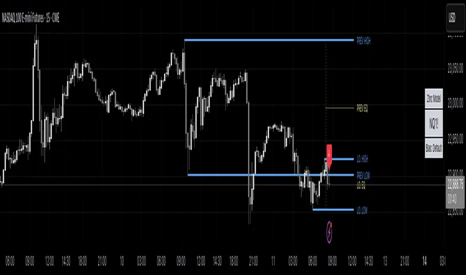
Zinc Model [Mr Zinc x MMT]The Zinc Model is a TradingView indicator designed to assist traders by plotting key price levels from two defined trading sessions: the previous day's session (4:00 AM to 8:00 PM) and the current day's London session (4:00 AM to 9:15 AM). It overlays horizontal lines for session highs, lows, and midpoints (EQ levels), along with a vertical anchor line to mark session starts. The indicator is highly customizable, allowing traders to tailor its appearance and focus on specific sessions for strategic analysis.
Features
Session-Based Levels : Tracks and displays high, low, and midpoint (50% EQ) levels for two sessions: the previous day's session and the current day's London session.
Customizable Display : Users can toggle visibility of high, low, EQ levels, and session anchor lines, with options to adjust line styles, colors, and widths.
Session Selection : Configurable session show times (default: 8:00 AM to 4:00 PM in New York time) for displaying levels, with a projection offset to extend lines into future bars.
Labels: Optional labels for each level (High, Low, EQ) with customizable sizes (Tiny, Small, Normal, Large) for clear identification.
Time Zone Support : Anchors sessions to a specified time zone (default: America/New_York).
How It Works
The indicator calculates key price levels based on two user-defined sessions:
- Previous Day Session (4:00 AM–8:00 PM) : Tracks the high, low, and midpoint (50% of the range) of the previous day's session.
- London Session (4:00 AM–9:15 AM) : Tracks the high, low, and midpoint of the current day's London session.
- Levels Displayed :
High/Low Levels : Horizontal lines at the highest and lowest prices of each session.
EQ Level : A horizontal line at the 50% midpoint of the session's range.
Anchor Line : A vertical line marking the start of the user-defined display session.
- Levels are plotted during a user-specified "Show Session" time window (default: 8:00 AM–4:00 PM) and extended forward by a configurable number of bars (default: 15).
- The indicator updates dynamically as new highs or lows occur within the active session.
Usage
- Add to Chart : Apply the indicator to any TradingView chart.
- Configure Settings :
Session Settings : Adjust the "Session Show Time" (default: 8:00 AM–4:00 PM) and time zone to align with your trading strategy.
Projection Offset : Set the number of bars to extend level lines into the future.
Anchor Line : Toggle the vertical line at session start and customize its style, color, and width.
High/Low/EQ Levels : Enable or disable lines and labels for each session's high, low, and midpoint, and customize their appearance.
Label Size : Choose from Tiny, Small, Normal, or Large for level labels.
- Interpret Levels :
High/Low Lines : Act as potential resistance (high) or support (low) levels.
EQ Line : Represents the session's midpoint, often a pivot point for price action.
Anchor Line : Marks the start of the display session for context.
- Trading Application : Use levels to identify support/resistance zones, set entry/exit points, or confirm breakouts during the specified session.
Settings
- Session Settings :
Session Show Time : Defines when levels are displayed (default: 8:00 AM–4:00 PM).
Projection Offset : Extends lines forward (default: 15 bars).
Time Zone : Sets the session time zone (default: America/New_York).
- Anchor Line Settings : Toggle visibility, style (Solid, Dashed, Dotted), color, and width.
- High/Low/EQ Settings : Separate controls for previous day and London sessions to toggle visibility, adjust line styles (Solid, Dashed, Dotted), colors, widths, and label visibility.
- Label Size : Options for Tiny, Small, Normal, or Large to adjust label appearance.
Ideal Use Case
The Zinc Model is ideal for day traders and swing traders focusing on session-based price action, particularly those trading forex, indices, or other markets with significant activity during the London session. It helps identify key support, resistance, and pivot levels for intraday strategies, with flexible settings to suit various timeframes and trading styles.
Smart LevelsSmart Levels - Professional Support & Resistance Indicator
🔥 ADVANCED TRUE OPENS & HIGH/LOW DETECTION SYSTEM
Smart Levels is a comprehensive technical analysis tool designed for professional traders who demand precision in identifying key market levels across multiple timeframes. This indicator automatically detects and displays critical support and resistance levels based on institutional trading concepts.
🎯 KEY FEATURES
TRUE OPENS DETECTION
Annual True Open: April 1st market opening (Q2 institutional cycle start)
Monthly Q1 & Q2 True Opens: First and second Monday of each month (customizable hours: 18:00 NY or 00:00 NY)
Weekly True Open: Every Monday at 18:00 NY (institutional week start)
Daily True Open: Midnight NY time (00:00 NY)
HIGH/LOW LEVELS IDENTIFICATION
Daily Highs & Lows: Previous day's extreme levels
Weekly Highs & Lows: Previous week's extreme levels
Monthly Highs & Lows: Previous month's extreme levels
Quarterly Highs & Lows: Previous quarter's extreme levels
Annual Highs & Lows: Previous year's extreme levels
ADVANCED CUSTOMIZATION
Master Controls: Enable/disable entire groups with one click
⚙️ Auto Scale Adjustment: Keep chart focused on price action (lines don't compress the view)
Individual Control: Each level can be configured independently
Line Styles: Solid, dashed, or dotted lines
Extension Types: Fixed displacement or last candle alignment
Color Coding: Fully customizable colors for each timeframe
PROFESSIONAL DISPLAY
Information Table: Live quarterly cycle status with color coding
Smart Labels: Price levels clearly marked with descriptive text
Multiple Positioning: Table can be positioned anywhere on chart
Clean Interface: Professional appearance with customizable text sizes
📊 INSTITUTIONAL CONCEPTS
This indicator is built on institutional trading principles:
Q1 (Accumulation): Smart money accumulation phase
Q2 (Manipulation): Price manipulation and liquidity hunting
Q3 (Distribution): Smart money distribution phase
Q4 (Continuation/Reversal): Trend continuation or major reversal
⚡ MASTER CONTROLS
🔥 DISPLAY ALL TRUE OPENS
Toggle all True Open levels on/off with a single click
📊 DISPLAY ALL HIGHS & LOWS
Toggle all High/Low levels on/off with a single click
⚙️ AUTO SCALE ADJUSTMENT (NEW FEATURE)
ON: Lines extend but don't affect chart scaling (maintains focus on price action)
OFF: Traditional behavior (lines may compress chart view)
Default: ENABLED for optimal trading experience
🛠 CONFIGURATION OPTIONS
True Open Settings (Per Timeframe)
Enable/Disable individual True Opens
Hour selection for monthly levels (18:00 NY or 00:00 NY)
Extension type: Fixed displacement or last candle alignment
Line appearance: Color, style, and width
Maximum number of lines displayed
High/Low Settings (Per Timeframe)
Enable/Disable individual High/Low pairs
Extension configuration
Separate colors for highs and lows
Line styling options
Information Table
Show/Hide information panel
Detailed view toggle
Position selection (6 options)
Text and background color customization
Text size adjustment
🎨 VISUAL FEATURES
Color-Coded Quarters: Each quarterly phase has distinct colors
Smart Positioning: Lines extend 20 candles beyond current price for clarity
Professional Labels: Clean price level identification
Memory Efficient: Automatic cleanup of old levels
Multi-Timeframe: Works on all timeframes from 1-minute to monthly
💡 TRADING APPLICATIONS
Support & Resistance
Previous High/Low levels act as natural S&R zones
True Opens often become significant pivot points
Institutional Analysis
Track quarterly cycles for macro trend analysis
Identify accumulation and distribution phases
Entry & Exit Points
Use level breaks for entry signals
Set targets at next timeframe levels
Risk Management
Place stops beyond key institutional levels
Size positions based on level confluence
🔧 TECHNICAL SPECIFICATIONS
Pine Script Version: v6
Overlay: Yes (displays directly on price chart)
Max Objects: 500 lines, 500 labels, 500 boxes
Timezone: America/New_York (institutional standard)
Performance: Optimized for all chart timeframes
Compatibility: Works with all TradingView accounts
📈 RECOMMENDED USAGE
Enable Master Controls for full functionality
Keep Auto Scale ON for optimal chart viewing
Customize colors to match your trading style
Use Information Table to track current quarterly phase
Combine with price action for high-probability setups
Smart Levels transforms complex institutional concepts into clear, actionable visual information. Whether you're scalping intraday moves or analyzing long-term trends, this indicator provides the precision levels professional traders depend on.
📊 Trade with institutional precision. Trade with Smart Levels.Tentar novamenteO Claude pode cometer erros. Confira sempre as respostas.Pesquisa Sonnet 4

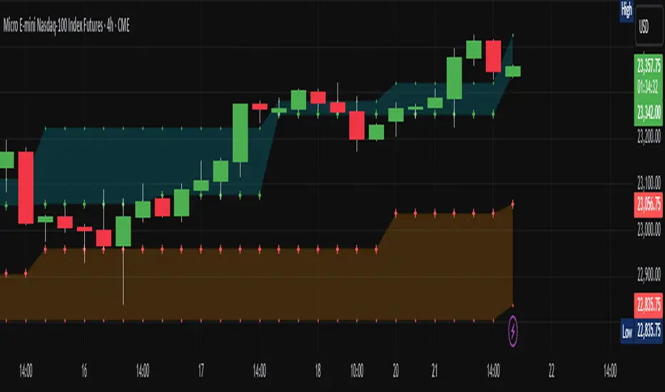
Initial balance - weeklyWeekly Initial Balance (IB) — Indicator Description
The Weekly Initial Balance (IB) is the price range (High–Low) established during the week’s first trading session (most commonly Monday). You can measure it over the entire day or just the first X hours (e.g. 60 or 120 minutes). Once that session ends, the IB High and IB Low define the key levels where the initial weekly range formed.
Why Measure the Weekly IB?
Week-Opening Sentiment:
Monday’s range often sets the tone for the rest of the week. Trading above the IB High signals bullish control; trading below the IB Low signals bearish control.
Key Liquidity Zones:
Large institutions tend to place orders around these extremes, so you’ll frequently see tests, breakouts, or rejections at these levels.
Support & Resistance:
The IB High and IB Low become natural barriers. Price will often return to them, bounce off them, or break through them—ideal spots for entries and exits.
Volatility Forecast:
The width of the IB (High minus Low) indicates whether to expect a volatile week (wide IB) or a quieter one (narrow IB).
Significance of IB Levels
Breakout:
A clear break above the IB High (for longs) or below the IB Low (for shorts) can ignite a strong trending move.
Fade:
A rejection off the IB High/Low during low momentum (e.g. low volume or pin-bar formations) offers a high-probability reversal trade.
Mid-Point:
The 50% level of the IB range often “magnetizes” price back to it, providing entry points for continuation or reversal strategies.
Three Core Monday IB Strategies
A. Breakout (Open-Range Breakout)
Entry: Wait for 1–2 candles (e.g. 5-minute) to close above IB High (long) or below IB Low (short).
Stop-Loss: A few pips below IB High (long) or above IB Low (short).
Profit-Target: 2–3× your risk (Reward:Risk ≥ 2:1).
Best When: You spot a clear impulse—such as a strong pre-open volume spike or news-driven move.
B. Fade (Reversal at Extremes)
Entry: When price tests IB High but shows weakening momentum (shrinking volume, upper-wick candles), enter short; vice versa for IB Low and longs.
Stop-Loss: Just beyond the IB extreme you’re fading.
Profit-Target: Back toward the IB mid-point (50% level) or all the way to the opposite IB extreme.
Best When: Monday’s action is range-bound and lacks a clear directional trend.
C. Mid-Point Trading
Entry: When price returns to the 50% level of the IB range.
In an up-trend: buy if it bounces off mid-point back toward IB High.
In a down-trend: sell if it reverses off mid-point back toward IB Low.
Stop-Loss: Just below the nearest swing-low (for longs) or above the nearest swing-high (for shorts).
Profit-Target: To the corresponding IB extreme (High or Low).
Best When: You see a strong initial move away from the IB, followed by a pullback to the mid-point.
Usage Steps
Configure your session: Measure IB over your chosen Monday timeframe (whole day or first X hours).
Choose your strategy: Align Breakout, Fade, or Mid-Point entries with the current market context (trend vs. range).
Manage risk: Keep risk per trade ≤ 1% of account and maintain at least a 2:1 Reward:Risk ratio.
Backtest & forward-test: Verify performance over multiple Mondays and in a paper-trading environment before going live.

Trend Gauge [BullByte]Trend Gauge
Summary
A multi-factor trend detection indicator that aggregates EMA alignment, VWMA momentum scaling, volume spikes, ATR breakout strength, higher-timeframe confirmation, ADX-based regime filtering, and RSI pivot-divergence penalty into one normalized trend score. It also provides a confidence meter, a Δ Score momentum histogram, divergence highlights, and a compact, scalable dashboard for at-a-glance status.
________________________________________
## 1. Purpose of the Indicator
Why this was built
Traders often monitor several indicators in parallel - EMAs, volume signals, volatility breakouts, higher-timeframe trends, ADX readings, divergence alerts, etc., which can be cumbersome and sometimes contradictory. The “Trend Gauge” indicator was created to consolidate these complementary checks into a single, normalized score that reflects the prevailing market bias (bullish, bearish, or neutral) and its strength. By combining multiple inputs with an adaptive regime filter, scaling contributions by magnitude, and penalizing weakening signals (divergence), this tool aims to reduce noise, highlight genuine trend opportunities, and warn when momentum fades.
Key Design Goals
Signal Aggregation
Merged trend-following signals (EMA crossover, ATR breakout, higher-timeframe confirmation) and momentum signals (VWMA thrust, volume spikes) into a unified score that reflects directional bias more holistically.
Market Regime Awareness
Implemented an ADX-style filter to distinguish between trending and ranging markets, reducing the influence of trend signals during sideways phases to avoid false breakouts.
Magnitude-Based Scaling
Replaced binary contributions with scaled inputs: VWMA thrust and ATR breakout are weighted relative to recent averages, allowing for more nuanced score adjustments based on signal strength.
Momentum Divergence Penalty
Integrated pivot-based RSI divergence detection to slightly reduce the overall score when early signs of momentum weakening are detected, improving risk-awareness in entries.
Confidence Transparency
Added a live confidence metric that shows what percentage of enabled sub-indicators currently agree with the overall bias, making the scoring system more interpretable.
Momentum Acceleration Visualization
Plotted the change in score (Δ Score) as a histogram bar-to-bar, highlighting whether momentum is increasing, flattening, or reversing, aiding in more timely decision-making.
Compact Informational Dashboard
Presented a clean, scalable dashboard that displays each component’s status, the final score, confidence %, detected regime (Trending/Ranging), and a labeled strength gauge for quick visual assessment.
________________________________________
## 2. Why a Trader Should Use It
Main benefits and use cases
1. Unified View: Rather than juggling multiple windows or panels, this indicator delivers a single score synthesizing diverse signals.
2. Regime Filtering: In ranging markets, trend signals often generate false entries. The ADX-based regime filter automatically down-weights trend-following components, helping you avoid chasing false breakouts.
3. Nuanced Momentum & Volatility: VWMA and ATR breakout contributions are normalized by recent averages, so strong moves register strongly while smaller fluctuations are de-emphasized.
4. Early Warning of Weakening: Pivot-based RSI divergence is detected and used to slightly reduce the score when price/momentum diverges, giving a cautionary signal before a full reversal.
5. Confidence Meter: See at a glance how many sub-indicators align with the aggregated bias (e.g., “80% confidence” means 4 out of 5 components agree ). This transparency avoids black-box decisions.
6. Trend Acceleration/Deceleration View: The Δ Score histogram visualizes whether the aggregated score is rising (accelerating trend) or falling (momentum fading), supplementing the main oscillator.
7. Compact Dashboard: A corner table lists each check’s status (“Bull”, “Bear”, “Flat” or “Disabled”), plus overall Score, Confidence %, Regime, Trend Strength label, and a gauge bar. Users can scale text size (Normal, Small, Tiny) without removing elements, so the full picture remains visible even in compact layouts.
8. Customizable & Transparent: All components can be enabled/disabled and parameterized (lengths, thresholds, weights). The full Pine code is open and well-commented, letting users inspect or adapt the logic.
9. Alert-ready: Built-in alert conditions fire when the score crosses weak thresholds to bullish/bearish or returns to neutral, enabling timely notifications.
________________________________________
## 3. Component Rationale (“Why These Specific Indicators?”)
Each sub-component was chosen because it adds complementary information about trend or momentum:
1. EMA Cross
o Basic trend measure: compares a faster EMA vs. a slower EMA. Quickly reflects trend shifts but by itself can whipsaw in sideways markets.
2. VWMA Momentum
o Volume-weighted moving average change indicates momentum with volume context. By normalizing (dividing by a recent average absolute change), we capture the strength of momentum relative to recent history. This scaling prevents tiny moves from dominating and highlights genuinely strong momentum.
3. Volume Spikes
o Sudden jumps in volume combined with price movement often accompany stronger moves or reversals. A binary detection (+1 for bullish spike, -1 for bearish spike) flags high-conviction bars.
4. ATR Breakout
o Detects price breaking beyond recent highs/lows by a multiple of ATR. Measures breakout strength by how far beyond the threshold price moves relative to ATR, capped to avoid extreme outliers. This gives a volatility-contextual trend signal.
5. Higher-Timeframe EMA Alignment
o Confirms whether the shorter-term trend aligns with a higher timeframe trend. Uses request.security with lookahead_off to avoid future data. When multiple timeframes agree, confidence in direction increases.
6. ADX Regime Filter (Manual Calculation)
o Computes directional movement (+DM/–DM), smoothes via RMA, computes DI+ and DI–, then a DX and ADX-like value. If ADX ≥ threshold, market is “Trending” and trend components carry full weight; if ADX < threshold, “Ranging” mode applies a configurable weight multiplier (e.g., 0.5) to trend-based contributions, reducing false signals in sideways conditions. Volume spikes remain binary (optional behavior; can be adjusted if desired).
7. RSI Pivot-Divergence Penalty
o Uses ta.pivothigh / ta.pivotlow with a lookback to detect pivot highs/lows on price and corresponding RSI values. When price makes a higher high but RSI makes a lower high (bearish divergence), or price makes a lower low but RSI makes a higher low (bullish divergence), a divergence signal is set. Rather than flipping the trend outright, the indicator subtracts (or adds) a small penalty (configurable) from the aggregated score if it would weaken the current bias. This subtle adjustment warns of weakening momentum without overreacting to noise.
8. Confidence Meter
o Counts how many enabled components currently agree in direction with the aggregated score (i.e., component sign × score sign > 0). Displays this as a percentage. A high percentage indicates strong corroboration; a low percentage warns of mixed signals.
9. Δ Score Momentum View
o Plots the bar-to-bar change in the aggregated score (delta_score = score - score ) as a histogram. When positive, bars are drawn in green above zero; when negative, bars are drawn in red below zero. This reveals acceleration (rising Δ) or deceleration (falling Δ), supplementing the main oscillator.
10. Dashboard
• A table in the indicator pane’s top-right with 11 rows:
1. EMA Cross status
2. VWMA Momentum status
3. Volume Spike status
4. ATR Breakout status
5. Higher-Timeframe Trend status
6. Score (numeric)
7. Confidence %
8. Regime (“Trending” or “Ranging”)
9. Trend Strength label (e.g., “Weak Bullish Trend”, “Strong Bearish Trend”)
10. Gauge bar visually representing score magnitude
• All rows always present; size_opt (Normal, Small, Tiny) only changes text size via text_size, not which elements appear. This ensures full transparency.
________________________________________
## 4. What Makes This Indicator Stand Out
• Regime-Weighted Multi-Factor Score: Trend and momentum signals are adaptively weighted by market regime (trending vs. ranging) , reducing false signals.
• Magnitude Scaling: VWMA and ATR breakout contributions are normalized by recent average momentum or ATR, giving finer gradation compared to simple ±1.
• Integrated Divergence Penalty: Divergence directly adjusts the aggregated score rather than appearing as a separate subplot; this influences alerts and trend labeling in real time.
• Confidence Meter: Shows the percentage of sub-signals in agreement, providing transparency and preventing blind trust in a single metric.
• Δ Score Histogram Momentum View: A histogram highlights acceleration or deceleration of the aggregated trend score, helping detect shifts early.
• Flexible Dashboard: Always-visible component statuses and summary metrics in one place; text size scaling keeps the full picture available in cramped layouts.
• Lookahead-Safe HTF Confirmation: Uses lookahead_off so no future data is accessed from higher timeframes, avoiding repaint bias.
• Repaint Transparency: Divergence detection uses pivot functions that inherently confirm only after lookback bars; description documents this lag so users understand how and when divergence labels appear.
• Open-Source & Educational: Full, well-commented Pine v6 code is provided; users can learn from its structure: manual ADX computation, conditional plotting with series = show ? value : na, efficient use of table.new in barstate.islast, and grouped inputs with tooltips.
• Compliance-Conscious: All plots have descriptive titles; inputs use clear names; no unnamed generic “Plot” entries; manual ADX uses RMA; all request.security calls use lookahead_off. Code comments mention repaint behavior and limitations.
________________________________________
## 5. Recommended Timeframes & Tuning
• Any Timeframe: The indicator works on small (e.g., 1m) to large (daily, weekly) timeframes. However:
o On very low timeframes (<1m or tick charts), noise may produce frequent whipsaws. Consider increasing smoothing lengths, disabling certain components (e.g., volume spike if volume data noisy), or using a larger pivot lookback for divergence.
o On higher timeframes (daily, weekly), consider longer lookbacks for ATR breakout or divergence, and set Higher-Timeframe trend appropriately (e.g., 4H HTF when on 5 Min chart).
• Defaults & Experimentation: Default input values are chosen to be balanced for many liquid markets. Users should test with replay or historical analysis on their symbol/timeframe and adjust:
o ADX threshold (e.g., 20–30) based on instrument volatility.
o VWMA and ATR scaling lengths to match average volatility cycles.
o Pivot lookback for divergence: shorter for faster markets, longer for slower ones.
• Combining with Other Analysis: Use in conjunction with price action, support/resistance, candlestick patterns, order flow, or other tools as desired. The aggregated score and alerts can guide attention but should not be the sole decision-factor.
________________________________________
## 6. How Scoring and Logic Works (Step-by-Step)
1. Compute Sub-Scores
o EMA Cross: Evaluate fast EMA > slow EMA ? +1 : fast EMA < slow EMA ? -1 : 0.
o VWMA Momentum: Calculate vwma = ta.vwma(close, length), then vwma_mom = vwma - vwma . Normalize: divide by recent average absolute momentum (e.g., ta.sma(abs(vwma_mom), lookback)), clip to .
o Volume Spike: Compute vol_SMA = ta.sma(volume, len). If volume > vol_SMA * multiplier AND price moved up ≥ threshold%, assign +1; if moved down ≥ threshold%, assign -1; else 0.
o ATR Breakout: Determine recent high/low over lookback. If close > high + ATR*mult, compute distance = close - (high + ATR*mult), normalize by ATR, cap at a configured maximum. Assign positive contribution. Similarly for bearish breakout below low.
o Higher-Timeframe Trend: Use request.security(..., lookahead=barmerge.lookahead_off) to fetch HTF EMAs; assign +1 or -1 based on alignment.
2. ADX Regime Weighting
o Compute manual ADX: directional movements (+DM, –DM), smoothed via RMA, DI+ and DI–, then DX and ADX via RMA. If ADX ≥ threshold, market is considered “Trending”; otherwise “Ranging.”
o If trending, trend-based contributions (EMA, VWMA, ATR, HTF) use full weight = 1.0. If ranging, use weight = ranging_weight (e.g., 0.5) to down-weight them. Volume spike stays binary ±1 (optional to change if desired).
3. Aggregate Raw Score
o Sum weighted contributions of all enabled components. Count the number of enabled components; if zero, default count = 1 to avoid division by zero.
4. Divergence Penalty
o Detect pivot highs/lows on price and corresponding RSI values, using a lookback. When price and RSI diverge (bearish or bullish divergence), check if current raw score is in the opposing direction:
If bearish divergence (price higher high, RSI lower high) and raw score currently positive, subtract a penalty (e.g., 0.5).
If bullish divergence (price lower low, RSI higher low) and raw score currently negative, add a penalty.
o This reduces score magnitude to reflect weakening momentum, without flipping the trend outright.
5. Normalize and Smooth
o Normalized score = (raw_score / number_of_enabled_components) * 100. This yields a roughly range.
o Optional EMA smoothing of this normalized score to reduce noise.
6. Interpretation
o Sign: >0 = net bullish bias; <0 = net bearish bias; near zero = neutral.
o Magnitude Zones: Compare |score| to thresholds (Weak, Medium, Strong) to label trend strength (e.g., “Weak Bullish Trend”, “Medium Bearish Trend”, “Strong Bullish Trend”).
o Δ Score Histogram: The histogram bars from zero show change from previous bar’s score; positive bars indicate acceleration, negative bars indicate deceleration.
o Confidence: Percentage of sub-indicators aligned with the score’s sign.
o Regime: Indicates whether trend-based signals are fully weighted or down-weighted.
________________________________________
## 7. Oscillator Plot & Visualization: How to Read It
Main Score Line & Area
The oscillator plots the aggregated score as a line, with colored fill: green above zero for bullish area, red below zero for bearish area. Horizontal reference lines at ±Weak, ±Medium, and ±Strong thresholds mark zones: crossing above +Weak suggests beginning of bullish bias, above +Medium for moderate strength, above +Strong for strong trend; similarly for bearish below negative thresholds.
Δ Score Histogram
If enabled, a histogram shows score - score . When positive, bars appear in green above zero, indicating accelerating bullish momentum; when negative, bars appear in red below zero, indicating decelerating or reversing momentum. The height of each bar reflects the magnitude of change in the aggregated score from the prior bar.
Divergence Highlight Fill
If enabled, when a pivot-based divergence is confirmed:
• Bullish Divergence : fill the area below zero down to –Weak threshold in green, signaling potential reversal from bearish to bullish.
• Bearish Divergence : fill the area above zero up to +Weak threshold in red, signaling potential reversal from bullish to bearish.
These fills appear with a lag equal to pivot lookback (the number of bars needed to confirm the pivot). They do not repaint after confirmation, but users must understand this lag.
Trend Direction Label
When score crosses above or below the Weak threshold, a small label appears near the score line reading “Bullish” or “Bearish.” If the score returns within ±Weak, the label “Neutral” appears. This helps quickly identify shifts at the moment they occur.
Dashboard Panel
In the indicator pane’s top-right, a table shows:
1. EMA Cross status: “Bull”, “Bear”, “Flat”, or “Disabled”
2. VWMA Momentum status: similarly
3. Volume Spike status: “Bull”, “Bear”, “No”, or “Disabled”
4. ATR Breakout status: “Bull”, “Bear”, “No”, or “Disabled”
5. Higher-Timeframe Trend status: “Bull”, “Bear”, “Flat”, or “Disabled”
6. Score: numeric value (rounded)
7. Confidence: e.g., “80%” (colored: green for high, amber for medium, red for low)
8. Regime: “Trending” or “Ranging” (colored accordingly)
9. Trend Strength: textual label based on magnitude (e.g., “Medium Bullish Trend”)
10. Gauge: a bar of blocks representing |score|/100
All rows remain visible at all times; changing Dashboard Size only scales text size (Normal, Small, Tiny).
________________________________________
## 8. Example Usage (Illustrative Scenario)
Example: BTCUSD 5 Min
1. Setup: Add “Trend Gauge ” to your BTCUSD 5 Min chart. Defaults: EMAs (8/21), VWMA 14 with lookback 3, volume spike settings, ATR breakout 14/5, HTF = 5m (or adjust to 4H if preferred), ADX threshold 25, ranging weight 0.5, divergence RSI length 14 pivot lookback 5, penalty 0.5, smoothing length 3, thresholds Weak=20, Medium=50, Strong=80. Dashboard Size = Small.
2. Trend Onset: At some point, price breaks above recent high by ATR multiple, volume spikes upward, faster EMA crosses above slower EMA, HTF EMA also bullish, and ADX (manual) ≥ threshold → aggregated score rises above +20 (Weak threshold) into +Medium zone. Dashboard shows “Bull” for EMA, VWMA, Vol Spike, ATR, HTF; Score ~+60–+70; Confidence ~100%; Regime “Trending”; Trend Strength “Medium Bullish Trend”; Gauge ~6–7 blocks. Δ Score histogram bars are green and rising, indicating accelerating bullish momentum. Trader notes the alignment.
3. Divergence Warning: Later, price makes a slightly higher high but RSI fails to confirm (lower RSI high). Pivot lookback completes; the indicator highlights a bearish divergence fill above zero and subtracts a small penalty from the score, causing score to stall or retrace slightly. Dashboard still bullish but score dips toward +Weak. This warns the trader to tighten stops or take partial profits.
4. Trend Weakens: Score eventually crosses below +Weak back into neutral; a “Neutral” label appears, and a “Neutral Trend” alert fires if enabled. Trader exits or avoids new long entries. If score subsequently crosses below –Weak, a “Bearish” label and alert occur.
5. Customization: If the trader finds VWMA noise too frequent on this instrument, they may disable VWMA or increase lookback. If ATR breakouts are too rare, adjust ATR length or multiplier. If ADX threshold seems off, tune threshold. All these adjustments are explained in Inputs section.
6. Visualization: The screenshot shows the main score oscillator with colored areas, reference lines at ±20/50/80, Δ Score histogram bars below/above zero, divergence fill highlighting potential reversal, and the dashboard table in the top-right.
________________________________________
## 9. Inputs Explanation
A concise yet clear summary of inputs helps users understand and adjust:
1. General Settings
• Theme (Dark/Light): Choose background-appropriate colors for the indicator pane.
• Dashboard Size (Normal/Small/Tiny): Scales text size only; all dashboard elements remain visible.
2. Indicator Settings
• Enable EMA Cross: Toggle on/off basic EMA alignment check.
o Fast EMA Length and Slow EMA Length: Periods for EMAs.
• Enable VWMA Momentum: Toggle VWMA momentum check.
o VWMA Length: Period for VWMA.
o VWMA Momentum Lookback: Bars to compare VWMA to measure momentum.
• Enable Volume Spike: Toggle volume spike detection.
o Volume SMA Length: Period to compute average volume.
o Volume Spike Multiplier: How many times above average volume qualifies as spike.
o Min Price Move (%): Minimum percent change in price during spike to qualify as bullish or bearish.
• Enable ATR Breakout: Toggle ATR breakout detection.
o ATR Length: Period for ATR.
o Breakout Lookback: Bars to look back for recent highs/lows.
o ATR Multiplier: Multiplier for breakout threshold.
• Enable Higher Timeframe Trend: Toggle HTF EMA alignment.
o Higher Timeframe: E.g., “5” for 5-minute when on 1-minute chart, or “60” for 5 Min when on 15m, etc. Uses lookahead_off.
• Enable ADX Regime Filter: Toggles regime-based weighting.
o ADX Length: Period for manual ADX calculation.
o ADX Threshold: Value above which market considered trending.
o Ranging Weight Multiplier: Weight applied to trend components when ADX < threshold (e.g., 0.5).
• Scale VWMA Momentum: Toggle normalization of VWMA momentum magnitude.
o VWMA Mom Scale Lookback: Period for average absolute VWMA momentum.
• Scale ATR Breakout Strength: Toggle normalization of breakout distance by ATR.
o ATR Scale Cap: Maximum multiple of ATR used for breakout strength.
• Enable Price-RSI Divergence: Toggle divergence detection.
o RSI Length for Divergence: Period for RSI.
o Pivot Lookback for Divergence: Bars on each side to identify pivot high/low.
o Divergence Penalty: Amount to subtract/add to score when divergence detected (e.g., 0.5).
3. Score Settings
• Smooth Score: Toggle EMA smoothing of normalized score.
• Score Smoothing Length: Period for smoothing EMA.
• Weak Threshold: Absolute score value under which trend is considered weak or neutral.
• Medium Threshold: Score above Weak but below Medium is moderate.
• Strong Threshold: Score above this indicates strong trend.
4. Visualization Settings
• Show Δ Score Histogram: Toggle display of the bar-to-bar change in score as a histogram. Default true.
• Show Divergence Fill: Toggle background fill highlighting confirmed divergences. Default true.
Each input has a tooltip in the code.
________________________________________
## 10. Limitations, Repaint Notes, and Disclaimers
10.1. Repaint & Lag Considerations
• Pivot-Based Divergence Lag: The divergence detection uses ta.pivothigh / ta.pivotlow with a specified lookback. By design, a pivot is only confirmed after the lookback number of bars. As a result:
o Divergence labels or fills appear with a delay equal to the pivot lookback.
o Once the pivot is confirmed and the divergence is detected, the fill/label does not repaint thereafter, but you must understand and accept this lag.
o Users should not treat divergence highlights as predictive signals without additional confirmation, because they appear after the pivot has fully formed.
• Higher-Timeframe EMA Alignment: Uses request.security(..., lookahead=barmerge.lookahead_off), so no future data from the higher timeframe is used. This avoids lookahead bias and ensures signals are based only on completed higher-timeframe bars.
• No Future Data: All calculations are designed to avoid using future information. For example, manual ADX uses RMA on past data; security calls use lookahead_off.
10.2. Market & Noise Considerations
• In very choppy or low-liquidity markets, some components (e.g., volume spikes or VWMA momentum) may be noisy. Users can disable or adjust those components’ parameters.
• On extremely low timeframes, noise may dominate; consider smoothing lengths or disabling certain features.
• On very high timeframes, pivots and breakouts occur less frequently; adjust lookbacks accordingly to avoid sparse signals.
10.3. Not a Standalone Trading System
• This is an indicator, not a complete trading strategy. It provides signals and context but does not manage entries, exits, position sizing, or risk management.
• Users must combine it with their own analysis, money management, and confirmations (e.g., price patterns, support/resistance, fundamental context).
• No guarantees: past behavior does not guarantee future performance.
10.4. Disclaimers
• Educational Purposes Only: The script is provided as-is for educational and informational purposes. It does not constitute financial, investment, or trading advice.
• Use at Your Own Risk: Trading involves risk of loss. Users should thoroughly test and use proper risk management.
• No Guarantees: The author is not responsible for trading outcomes based on this indicator.
• License: Published under Mozilla Public License 2.0; code is open for viewing and modification under MPL terms.
________________________________________
## 11. Alerts
• The indicator defines three alert conditions:
1. Bullish Trend: when the aggregated score crosses above the Weak threshold.
2. Bearish Trend: when the score crosses below the negative Weak threshold.
3. Neutral Trend: when the score returns within ±Weak after being outside.
Good luck
– BullByte

AI Strat ATR Dinamico + ADX + Trend Adaptivo (No Repaint)Below is a fully self-contained, English-language description of every input, function, and logical block inside the “AI Strat ATR Dinamico + ADX + Trend Adaptivo (No Repaint)” indicator. You can copy and paste this into TradingView’s “Description” field when you publish, without exposing any Pine code.
---
## Indicator Name and Purpose
**Name (Short Title):**
AI Strat Adaptive v3 (NoRepaint)
**Overview:**
This indicator combines multiple technical tools—RSI, EMA, ATR (with a dynamic multiplier), ADX/DI, and an “AI‐style” scoring mechanism—to generate trend-filtered and reversal signals. It also optionally confirms signals on a higher timeframe, dynamically adjusts its sensitivity based on volatility, and plots intrabar stop‐loss (SL) and take‐profit (TP) levels derived from ATR. Special care has been taken to ensure that no signals “repaint” (i.e., once drawn on a closed bar, they never disappear or shift).
---
## 1. Main Inputs
All of the inputs appear in the Settings dialog for the published indicator. Below is a detailed explanation of each input, grouped by logical category.
### A. RSI & EMA Base Parameters
1. **RSI Length (Base)**
* **Input type:** Integer (default 14)
* **Description:** Number of bars used to calculate the Relative Strength Index (RSI). A shorter RSI reacts more quickly to price changes; a longer RSI is smoother.
2. **RSI Overbought Threshold**
* **Input type:** Integer (default 60)
* **Description:** If the RSI value rises above this level, it contributes a “sell” signal component. You can adjust this (e.g., 70) to make your system more conservative.
3. **RSI Oversold Threshold**
* **Input type:** Integer (default 40)
* **Description:** If the RSI falls below this level, it contributes a “buy” signal component. Raising this threshold (e.g., 50) makes the strategy more aggressive in seeking reversals.
4. **EMA Length (Base)**
* **Input type:** Integer (default 20)
* **Description:** Number of bars for the Exponential Moving Average (EMA). A shorter EMA will produce more frequent crossovers, a longer EMA is smoother.
### B. ATR & Volatility Filter Parameters
5. **ATR Length (Base)**
* **Input type:** Integer (default 14)
* **Description:** Number of bars to calculate Average True Range (ATR). The ATR is used both for measuring volatility and for dynamic SL/TP levels.
6. **ATR SMA Length**
* **Input type:** Integer (default 50)
* **Description:** Number of bars to compute a Simple Moving Average of the ATR itself. This gives a baseline of “normal” volatility. If ATR rises significantly above this SMA, the indicator treats the market as “high volatility.”
7. **ATR Multiplier Base**
* **Input type:** Float (default 1.2, step 0.1)
* **Description:** Base multiplier for ATR when filtering for volatility. The actual threshold is computed as `ATR_SMA × (ATR_Multiplier Base) × sqrt(current_ATR / ATR_SMA)`. In other words, the multiplier becomes larger if volatility is rising, and smaller if volatility is falling.
8. **Disable Volatility Filter**
* **Input type:** Boolean (default false)
* **Description:** If enabled (true), the indicator will ignore any volatility‐based filtering, using signals regardless of ATR behavior. If disabled (false), signals only fire when ATR > (ATR\_SMA × dynamic multiplier).
### C. Price-Change & “AI Score” Parameters
9. **Price Change Period (bars)**
* **Input type:** Integer (default 3)
* **Description:** The number of bars back to measure percentage price change. Used to ensure that a “trend” signal is accompanied by a sufficiently positive (for longs) or negative (for shorts) price movement over this many bars.
10. **Base AI Score Threshold**
* **Input type:** Float (default 0.1)
* **Description:** The indicator computes a composite “AI-style” score by combining the RSI signal (overbought/oversold) and an EMA crossover signal. Only if the absolute value of that composite score exceeds this threshold will a trend signal be eligible. Raising it makes signals rarer but (potentially) higher-conviction.
### D. SMA “ICT” Trend Filter Parameters
11. **ICT SMA Long Length (Base)**
* **Input type:** Integer (default 50)
* **Description:** Number of bars for the “long” Simple Moving Average (SMA) used in the internal trend filter. Typically, price must be above this SMA (and ADX must be strong) to confirm an uptrend, or below it (and ADX strong) to confirm a downtrend.
12. **ICT SMA Short1 Length (Base)**
* **Input type:** Integer (default 10)
* **Description:** Secondary “fast” SMA used both for reversal logic (e.g., price crossing above it can count as a bullish reversal) and part of the internal trend confirmation.
13. **ICT SMA Short2 Length (Base)**
* **Input type:** Integer (default 20)
* **Description:** A second “medium” SMA used for reversal triggers (e.g., crossovers or crossunders alongside RSI conditions).
### E. ADX & DI Parameters
14. **Base ADX Length**
* **Input type:** Integer (default 14)
* **Description:** Number of bars for the ADX (Average Directional Index) moving averages, which measure trend strength. The same length is used for +DI and –DI smoothing.
15. **Base ADX Threshold**
* **Input type:** Float (default 25.0, step 0.5)
* **Description:** If ADX > this threshold and +DI > –DI, we consider an uptrend; if ADX > this threshold and –DI > +DI, we consider a downtrend. Raising this value demands stronger trends to qualify.
### F. Sensitivity & Cooldown
16. **Sensitivity (0–1)**
* **Input type:** Float between 0.0 and 1.0 (default 0.5)
* **Description:** A general “mixture” parameter used internally to weight how aggressively the indicator leans into trend versus reversal. In practice, the code uses it to fine-tune exact thresholds for switching between trend and reversal conditions. You can leave it at 0.5 unless you want to bias more heavily toward either regime.
17. **Base Cooldown Bars Between Signals**
* **Input type:** Integer (default 5, min 0)
* **Description:** Once a long or short signal fires, the indicator will wait at least this many bars before allowing a new signal in the same direction. Prevents “signal flipping” on each bar. A higher number forces fewer, more spaced-out entries.
18. **Trend Confirmation Bars**
* **Input type:** Integer (default 3, min 1)
* **Description:** After the directional filters (+DI/–DI cross, price vs. SMA), the indicator still requires that price remains on the same side of the long SMA for at least this many consecutive bars before confirming “trend up” or “trend down.” Larger values smooth out false breakouts but may lag signals.
### G. Higher Timeframe Confirmation
19. **Use Higher Timeframe Confirmation**
* **Input type:** Boolean (default true)
* **Description:** If true, the indicator will request a block of values (SMA, +DI, –DI, ADX) from a higher timeframe (default 60 minutes) and require that the higher timeframe is also in agreement (strong uptrend or strong downtrend) before confirming your current-timeframe trend. This helps filter out lower-timeframe noise.
20. **Higher Timeframe (TF) for Confirmation**
* **Input type:** Timeframe (default “60”)
* **Description:** The chart timeframe (e.g., 5, 15, 60 minutes) whose trend conditions must also be true. It’s sent through a `request.security(..., lookahead=barmerge.lookahead_off)` call so that it never “paints ahead.”
### H. Dynamic TP/SL Parameters
21. **TP as ATR Multiple**
* **Input type:** Float (default 2.0, step 0.1)
* **Description:** When a trade is open, the “take-profit” price is determined by looking at the highest high (for longs) or lowest low (for shorts) observed since entry, and then plotting a cross (“X”) at that level when the trend finally flips. This is purely for display. However, separate from that, this parameter can be adapted if you want a strictly ATR–based TP. In the “Minimal” version, TP is ≈ (highest high) once trend inverts, but you could rewrite it to use `entry_price + ATR×TP_Multiplier`.
22. **SL as ATR Multiple**
* **Input type:** Float (default 1.0, step 0.1)
* **Description:** While in a trade, a trailing SL line is plotted each bar. Its value is always `entry_price ± (ATR × SL_Multiplier)`. When the trend inverts, the SL no longer updates, and you see it on the chart.
### I. Display and Mode Options
23. **Show Debug Lines**
* **Input type:** Boolean (default true)
* **Description:** When enabled, the indicator will plot all intermediate lines—ATR SMA, ATR Threshold, +DI, –DI, ADX (current and HTF), HTF SMA, etc.—so that you can diagnose exactly what’s happening. Turn this off to hide all debug information and only see entry/exit shapes.
24. **Enable Scalping Mode**
* **Input type:** Boolean (default false)
* **Description:** If true, many of the “base” parameters are halved (e.g., RSI length becomes 7 instead of 14, ATR length becomes 7 instead of 14, ADX length becomes 7, etc.), and the ADX threshold is multiplied by 0.8. This makes all oscillators and moving averages more reactive, suited for very short-term (scalping) setups.
---
## 2. Core Calculation Blocks
Below is a high-level description of each logical block (in code order), translated from Pine into conceptual steps.
### A. Adjust Inputs if “Scalping Mode” Is On
If **Scalping Mode** = true, then:
* `RSI_Length` becomes `max(1, round(Base_RSI_Length / 2))`
* `EMA_Length` becomes `max(1, round(Base_EMA_Length / 2))`
* `ATR_Length` becomes `max(1, round(Base_ATR_Length / 2))`
* `Price_Change_Period` becomes `max(1, round(Base_Price_Change_Period / 2))`
* `SMA_Long_Length`, `SMA_Short1_Length`, and `SMA_Short2_Length` are each halved (minimum 1).
* `ADX_Length` = `max(1, round(Base_ADX_Length / 2))`
* `ADX_Threshold` = `Base_ADX_Threshold × 0.8`
* `Cooldown_Bars` = `max(0, round(Base_Cooldown_Bars / 2))`
Otherwise, all adjusted lengths = their base values.
### B. RSI, EMA & “AI Score” on Current Timeframe
1. **Compute RSI:**
* Uses the (possibly adjusted) `RSI_Length`.
* Denote this as `RSI_Value`.
2. **Compute ATR & Its SMA:**
* `ATR_Value` = `ta.atr(ATR_Length)`.
* `ATR_SMA` = `ta.sma(ATR_Value, ATR_SMA_Length)`.
* Then define `Volatility_Increase` = (`ATR_Value > ATR_SMA`).
* If the volatility has increased, the weighting of RSI vs. EMA changes.
3. **Compute Weights:**
* If `Volatility_Increase == true`, then:
* `RSI_Weight = 0.7`
* `EMA_Weight = 0.3`
* Otherwise:
* `RSI_Weight = 0.3`
* `EMA_Weight = 0.7`
4. **RSI Signal Component (`RSI_Sig`):**
* If `RSI_Value > RSI_Overbought`, then `RSI_Sig = –1`.
* Else if `RSI_Value < RSI_Oversold`, then `RSI_Sig = +1`.
* Otherwise, `RSI_Sig = 0`.
5. **EMA Value & Signal Component (`EMA_Sig`):**
* `EMA_Value` = `ta.ema(close, EMA_Length)`.
* `EMA_Sig = +1` if the current close crosses **above** the EMA; `EMA_Sig = –1` if the current close crosses **below** the EMA; else `0`.
6. **Compute Raw “AI Score”:**
$$
Raw\_AI = (RSI\_Sig \times RSI\_Weight)\;+\;(EMA\_Sig \times EMA\_Weight)
$$
Then,
$$
AI\_Score = \frac{Raw\_AI}{(RSI\_Weight + EMA\_Weight)}
$$
(This normalization ensures the score always ranges between –1 and +1 if both weights sum to 1.)
### C. Dynamic ATR Multiplier & Volatility Filter
1. **Volatility Factor:**
$$
Volatility\_Factor = \frac{ATR\_Value}{ATR\_SMA}
$$
2. **Dynamic ATR Multiplier:**
$$
ATR\_Multiplier = ATR\_Multiplier\_Base \times \sqrt{Volatility\_Factor}
$$
3. **High Volatility Condition (`High_Volatility`):**
* If `Disable_Volatility_Filter == true`, then treat `High_Volatility = true` always.
* Else, `High_Volatility = (ATR_Value > ATR_SMA × ATR_Multiplier)`.
### D. Price Change Percentage
* **Compute Price Change:**
$$
Price\_Change = \frac{(Close - Close )}{Close } \times 100
$$
* This is the percent return from `Price_Change_Period` bars ago to now.
* For a valid long‐trend signal, we require `Price_Change > 0`; for a short trend, `Price_Change < 0`.
### E. Local SMAs for Trend/Reversal Filters
* `SMA_Close_Long` = `ta.sma(close, SMA_Long_Length)`.
* `SMA_Close_Short1` = `ta.sma(close, SMA_Short1_Length)`.
* `SMA_Close_Short2` = `ta.sma(close, SMA_Short2_Length)`.
These three SMAs help define the “local trend” and reversal breakout points:
* **Primary Trend Filter:**
* Price must be above `SMA_Close_Long` for an uptrend filter, or below `SMA_Close_Long` for a downtrend filter.
* **Reversal Filter:**
* A bullish reversal is detected if **(RSI < Oversold AND close crosses above EMA)** OR **(RSI < Oversold AND close crosses above SMA\_Close\_Short1)**.
* A bearish reversal is detected if **(RSI > Overbought AND close crosses below EMA)** OR **(RSI > Overbought AND close crosses below SMA\_Close\_Short1)**.
### F. Manual +DI, –DI & ADX on Current Timeframe
Instead of relying on the built-in `ta.adx`, the script calculates DI and ADX manually. This makes it easier to replicate the exact logic on a higher timeframe via `request.security`. The steps are:
1. **Directional Movement (DM) Components:**
* `Up_Move` = `high – high `
* `Down_Move` = `low – low`
* `Plus_DM` = `Up_Move` if (`Up_Move > Down_Move` AND `Up_Move > 0`), else `0`
* `Minus_DM` = `Down_Move` if (`Down_Move > Up_Move` AND `Down_Move > 0`), else `0`
2. **True Range (TR) Components:**
* `TR1` = `high – low`
* `TR2` = `abs(high – close )`
* `TR3` = `abs(low – close )`
* `True_Range` = `max(TR1, TR2, TR3)`
3. **Smoothed Averages (RMA):**
* `Sm_TR` = `ta.rma(True_Range, ADX_Length)`
* `Sm_Plus` = `ta.rma(Plus_DM, ADX_Length)`
* `Sm_Minus`= `ta.rma(Minus_DM, ADX_Length)`
4. **Compute DI%:**
$$
Plus\_DI = \frac{Sm\_Plus}{Sm\_TR} \times 100,\quad
Minus\_DI = \frac{Sm\_Minus}{Sm\_TR} \times 100
$$
5. **DX and ADX:**
$$
DX = \frac{|Plus\_DI - Minus\_DI|}{Plus\_DI + Minus\_DI} \times 100,\quad
ADX = ta.rma(DX, ADX_Length)
$$
These values are referred to as `(plus_di, minus_di, adx_val)` for the current timeframe.
---
## 3. Higher Timeframe (HTF) Confirmation Function
If **Use Higher Timeframe Confirmation** is enabled, the script calls a single helper (Pine) function `f_htf` with two parameters: the ADX length and the SMA length (both taken from the “base” or “scaled” values). Internally, `f_htf` simply reruns the manual DI/ADX logic (same as above) on the higher timeframe’s bar data, and also includes that timeframe’s closing price and its SMA for trend comparison.
* **Request.Security Call:**
```
= request.security(
syminfo.tickerid,
higher_tf,
f_htf(adx_length, sma_long_len),
lookahead=barmerge.lookahead_off
)
```
* `lookahead=barmerge.lookahead_off` ensures that no HTF value “paints” early; you always see only confirmed HTF bars.
* The returned tuple provides:
1. `ht_close` = HTF closing price
2. `ht_sma` = HTF SMA of length `sma_long_len`
3. `ht_pdi` = HTF +DI percentage
4. `ht_mdi` = HTF –DI percentage
5. `ht_adx` = HTF ADX value
---
## 4. Trend & Reversal Filters (Current & HTF)
### A. Current-Timeframe Trend Filter
1. **Uptrend\_Basic (Current TF)**
$$
(plus\_di > minus\_di)\;\land\;(adx\_val > ADX\_Threshold)\;\land\;(close > SMA\_Close\_Long)
$$
2. **Downtrend\_Basic (Current TF)**
$$
(minus\_di > plus\_di)\;\land\;(adx\_val > ADX\_Threshold)\;\land\;(close < SMA\_Close\_Long)
$$
3. **Trend Confirmation by Bars:**
* `Bars_Since_Below` = number of bars since `close <= SMA_Close_Long`.
* `Bars_Since_Above` = number of bars since `close >= SMA_Close_Long`.
* If `Uptrend_Basic == true` AND `Bars_Since_Below ≥ Trend_Confirmation_Bars` → mark `Uptrend_Confirm = true`.
* If `Downtrend_Basic == true` AND `Bars_Since_Above ≥ Trend_Confirmation_Bars` → mark `Downtrend_Confirm = true`.
### B. Reversal Filters (Current TF)
1. **Bullish Reversal (`Rev_Bullish`):**
* If `(RSI < RSI_Oversold AND close crosses above EMA_Value)` OR
`(RSI < RSI_Oversold AND close crosses above SMA_Close_Short1)`
→ then `Rev_Bullish = true`.
2. **Bearish Reversal (`Rev_Bearish`):**
* If `(RSI > RSI_Overbought AND close crosses below EMA_Value)` OR
`(RSI > RSI_Overbought AND close crosses below SMA_Close_Short1)`
→ then `Rev_Bearish = true`.
### C. Higher-Timeframe Trend Filter (HTF)
1. **HTF Uptrend (`HT_Uptrend`):**
$$
(ht\_pdi > ht\_mdi)\;\land\;(ht\_adx > ADX\_Threshold)\;\land\;(ht\_close > ht\_sma)
$$
2. **HTF Downtrend (`HT_Downtrend`):**
$$
(ht\_mdi > ht\_pdi)\;\land\;(ht\_adx > ADX\_Threshold)\;\land\;(ht\_close < ht\_sma)
$$
3. **Combine Current & HTF:**
* If **Use\_HTF\_Confirmation == true**, then:
* `Uptrend_Confirm := Uptrend_Confirm AND HT_Uptrend`
* `Downtrend_Confirm := Downtrend_Confirm AND HT_Downtrend`
* Otherwise, just use the current timeframe’s `Uptrend_Confirm` and `Downtrend_Confirm`.
4. **Define `CurrentTrend` (Integer):**
* `CurrentTrend = +1` if `Uptrend_Confirm == true`.
* `CurrentTrend = –1` if `Downtrend_Confirm == true`.
* Otherwise, `CurrentTrend = 0`.
5. **Reset “One Trade Per Trend”:**
* There is a persistent variable `LastTradeTrend`.
* Every time `CurrentTrend` flips (i.e., `CurrentTrend != CurrentTrend `), the code sets `LastTradeTrend := 0`.
* That allows one new entry once the detected trend has changed.
---
## 5. One‐Time “Cooldown” Logic
* **`LastSignalBar`**
* A persistent integer (initially undefined).
* After each confirmed long or short entry, `LastSignalBar` is set to the bar index where that signal fired.
* **`Bars_Since_Signal`**
* If `LastSignalBar` is undefined, treat as a very large number (so that initial signals are always allowed).
* Otherwise, `Bars_Since_Signal = bar_index – LastSignalBar`.
* **Cooldown Check:**
* A new long (or short) can only be generated if `(Bars_Since_Signal > Signal_Cooldown)`.
* This prevents multiple signals in rapid succession.
---
## 6. Entry Conditions (No Repaint)
All of the conditions below are calculated “intrabar,” but the script only actually registers a **signal** on **bar close** (`barstate.isconfirmed`) so that signals never repaint.
### A. Trend‐Based “Raw” Conditions
1. **Trend\_Long\_Raw:**
$$
(AI\_Score > AI\_Score\_Threshold)\;\land\;Uptrend\_Confirm\;\land\;High\_Volatility\;\land\;(Price\_Change > 0)
$$
2. **Trend\_Short\_Raw:**
$$
(AI\_Score < -AI\_Score\_Threshold)\;\land\;Downtrend\_Confirm\;\land\;High\_Volatility\;\land\;(Price\_Change < 0)
$$
### B. Reversal “Raw” Conditions
1. **Rev\_Long\_Raw:**
$$
Rev\_Bullish\;\land\;(CurrentTrend \neq +1)
$$
2. **Rev\_Short\_Raw:**
$$
Rev\_Bearish\;\land\;(CurrentTrend \neq -1)
$$
### C. Combine Raw Signals
* `Raw_Long = Trend_Long_Raw OR Rev_Long_Raw`.
* `Raw_Short = Trend_Short_Raw OR Rev_Short_Raw`.
### D. Confirmed Long/Short Signal Flags
On each new bar **close** (`barstate.isconfirmed == true`):
* **Long\_Signal\_Confirmed** can fire if:
1. `Raw_Long == true`
2. `LastTradeTrend != +1` (we haven’t already taken a long in this same trend)
3. `Bars_Since_Signal > Signal_Cooldown`
If all three hold, then on this bar close the code sets:
* `Long_Signal = true`
* `LastTradeTrend := +1`
* `LastSignalBar := bar_index`
Otherwise, `Long_Signal := false` on this bar.
* **Short\_Signal\_Confirmed** works the same way but with `Raw_Short`, `LastTradeTrend != -1`, etc.
If triggered, it sets `Short_Signal = true`, `LastTradeTrend := -1`, and `LastSignalBar := bar_index`. Otherwise `Short_Signal := false`.
* **Important:** If the bar is still forming (`else` branch of `barstate.isconfirmed`), then both `Long_Signal` and `Short_Signal` are forced to `false`. This guarantees that no shape or alert appears until the bar actually closes.
---
## 7. Plotting Entry/Exit Shapes
1. **Trend Long Signal (Triangle Up)**
* Condition: `Long_Signal == true` **AND** `Trend_Long_Raw == true`.
* Appearance: A small, semi-transparent lime green triangle drawn **below** the bar.
2. **Trend Short Signal (Triangle Down)**
* Condition: `Short_Signal == true` **AND** `Trend_Short_Raw == true`.
* Appearance: A small, semi-transparent maroon triangle drawn **above** the bar.
3. **Reversal Long Signal (Circle)**
* Condition: `Long_Signal == true` **AND** `Rev_Long_Raw == true`.
* Appearance: A tiny, more transparent green circle drawn **below** the bar.
4. **Reversal Short Signal (Circle)**
* Condition: `Short_Signal == true` **AND** `Rev_Short_Raw == true`.
* Appearance: A tiny, more transparent red circle drawn **above** the bar.
Since `Long_Signal` and `Short_Signal` only ever become true at bar close, these shapes are never repainted or removed once drawn.
---
## 8. Unified Alert Message
* As soon as a new bar closes with either `Long_Signal` or `Short_Signal == true`, an alert message is sent:
* If `Long_Signal`, then `alert_msg = "action=BUY"`.
* If `Short_Signal`, then `alert_msg = "action=SELL"`.
* If neither, `alert_msg = ""` (no alert).
* The code calls `alert(alert_msg, freq=alert.freq_once_per_bar)` only if `barstate.isconfirmed` and `alert_msg` is non‐empty. This ensures exactly one alert per confirmed bar, no intrabar pops.
---
## 9. Dynamic TP/SL Logic (Minimal Implementation)
Once a long or short position is “open,” the script tracks these variables:
1. **Persistent Flags and Prices** (all persist between bars until reset):
* `InLong` (Boolean)
* `InShort` (Boolean)
* `Long_Max` (Float)
* `Short_Min` (Float)
* `Entry_Price` (Float)
2. **On Bar Close:**
* If `Long_Signal == true` →
* Set `InLong := true`,
* `Entry_Price := close` of that bar,
* `Long_Max := high ` (last bar’s high, so that we’re not using “future” data).
* If `Short_Signal == true` →
* Set `InShort := true`,
* `Entry_Price := close`,
* `Short_Min := low `.
3. **While `InLong == true`:**
* Continuously update `Long_Max = max(Long_Max, current high)` on each bar (intrabar, but finalized each close).
* Compute a dynamic SL:
$$
SL_{Long} = Entry\_Price - (ATR \times SL\_ATR\_Multiplier).
$$
* If **current trend** flips to non-uptrend (`CurrentTrend != +1`), mark `ExitLong = true`.
* Then the routine plots `TP_Long = Long_Max` as a cross (“X”) at that level.
* Set `InLong := false` so that no further changes to `Long_Max` or `Entry_Price` happen on future bars.
4. **While `InShort == true`:**
* Continuously update `Short_Min = min(Short_Min, current low)`.
* Compute a dynamic SL:
$$
SL_{Short} = Entry\_Price + (ATR \times SL\_ATR\_Multiplier).
$$
* If trend flips to non-downtrend (`CurrentTrend != –1`), mark `ExitShort = true`.
* Then the routine plots `TP_Short = Short_Min`.
* Set `InShort := false` to freeze those values.
5. **Plotting TP/SL if “Show Debug” is On:**
* **TP Shapes:**
* When `ExitLong == true`, plot a solid lime “X” at `TP_Long` (highest high).
* When `ExitShort == true`, plot a solid maroon “X” at `TP_Short` (lowest low).
* **SL Lines:**
* If still `InLong`, draw a thin red line at `SL_Long` on each bar.
* If still `InShort`, draw a thin green line at `SL_Short`.
Thus, your charts visually show the highest‐high take-profit cross for longs, the lowest-low take-profit cross for shorts, and a continuously updating trailing SL until the trend flips. Because all of this is triggered on confirmed bars, nothing “jumps around” after the fact.
---
## 10. Debug‐Only Plot Lines (When Enabled)
When **Show Debug Lines** = true, the indicator will also plot:
1. **ATR SMA (Orange):**
* The simple moving average of ATR over `ATR_SMA_Length`.
2. **ATR Threshold (Yellow):**
* `ATR_SMA × ATR_Multiplier` (the dynamically scaled threshold).
3. **+DI & –DI (Current TF):**
* +DI plotted as a green line, –DI plotted as a red line (opacity \~70%).
4. **ADX (Current TF, Blue):**
* A blue line for the present timeframe’s ADX.
5. **ADX Threshold (Gray):**
* A horizontal gray line showing `ADX_Threshold`.
6. **+DI & –DI (HTF, Darker Colors):**
* If HTF confirmation is on, “HTF +DI” is a greener but more transparent line; “HTF –DI” is a redder but more transparent line.
7. **ADX (HTF, Blue but Transparent):**
* HTF ADX plotted in blue (high transparency).
8. **HTF SMA (Orange, Transparent):**
* The higher timeframe’s SMA (same length as `SMA_Long_Length`), drawn in fainter orange.
9. **Volatility Zone Fill (Yellow Tinted Area):**
* Fills the area between `ATR_SMA` and `ATR_SMA × ATR_Multiplier`.
* Indicates “normal” versus “high‐volatility” regimes.
These debug lines are purely visual aids. Disable them if you want a cleaner chart.
---
## 11. Putting It All Together — Step-By-Step Flow
1. **Read Inputs** (RSI lengths, EMA length, ATR settings, etc.).
2. **Optionally Halve All Lengths** if “Scalping Mode” is checked.
3. **Calculate Current TF Indicators:**
* RSI, ATR, ATR\_SMA, EMA, price change, various SMAs, DI/ADX.
4. **Compute “AI Score”** (weighted sum of RSI and EMA signals).
5. **Compute Dynamic ATR Multiplier** and decide if “High Volatility” is true.
6. **Compute Raw Trend/Reversal Conditions** on the current timeframe (without triggering yet).
7. **Fetch HTF Values** in one `request.security` call (SMAs, DI/ADX).
8. **Combine Current & HTF Trend Filters** to confirm `Uptrend_Confirm` or `Downtrend_Confirm`.
9. **Check Reversal Conditions** (price crossing EMA or SMA short, in overbought/oversold zones).
10. **Enforce “One Trade Per Trend”** (clear `LastTradeTrend` whenever `CurrentTrend` flips).
11. **Enforce Cooldown** (must wait at least `Signal_Cooldown` bars since the prior signal).
12. **On Bar Close:**
* If `Raw_Long` AND not already in a long trend AND cooldown met, then fire `Long_Signal`.
* Else if `Raw_Short` AND not already in a short trend AND cooldown met, then fire `Short_Signal`.
* Otherwise, no new signal on this bar.
13. **Plot Long/Short Entry Shapes** according to whether it was a Trend signal or a Reversal signal.
14. **Send Alert** (“action=BUY” or “action=SELL”) exactly once per confirmed bar.
15. **If New Long/Short Signal, Set `InLong`/`InShort`, Record Entry Price, Initialize `Long_Max`/`Short_Min`.**
16. **While `InLong` is true:** Update `Long_Max = max(previous Long_Max, current high)`. Compute `SL_Long`. If the current trend flips (no longer uptrend), set `ExitLong = true`, plot a “TP X,” and close the position logic.
17. **While `InShort` is true:** Similarly update `Short_Min`, compute `SL_Short`, and if trend flips, set `ExitShort = true`, plot a “TP X,” and close the position logic.
18. **Optionally Display Debug Lines** (ATR SMA, ATR threshold, DI/ADX, HTF DI/ADX, etc.).
---
## 12. How to Use in TradingView Community
When you publish this indicator to the TradingView community—choosing “Protected” or “Invite-only” visibility—you can paste the above description into the “Description” field. Users will see exactly what each input does, how signals are generated, and what the various plotted lines represent, **without ever seeing the script source**. In this way, the code itself remains hidden but the logic is fully documented.
1. **Go to “Create New Indicator”** on TradingView.
2. **Paste Your Pine Code** (the full indicator script) in the Pine editor and save it.
3. **Set Visibility = Protected** (or Invite-only).
4. **In the “Description” Text Box, paste the entirety of this document** (steps 1–11).
5. **Click “Publish Script.”**
Users who view your indicator will see its name (“AI Strat Adaptive v3 (NoRepaint)”), a list of all inputs (with default values), and the detailed English description above. They can then load it on any chart, adjust inputs, and see the plotted signals, TP/SL lines, and optional debug overlays—without accessing the underlying Pine code.
---
### Summary of Key Points
* **RSI, EMA, ATR, DI/ADX, and “AI Score”** work together to define “trend vs. reversal.”
* **Dynamic volatility filter** uses ATR and ATR\_SMA to adapt the weighting of RSI vs. EMA and decide whether “volatility is high enough” to permit a trend trade.
* **One trade per detected trend** and a **cooldown period** prevent over‐trading.
* **Higher timeframe confirmation** (optional) further filters out noise.
* **No-repaint logic**:
* All signals only appear at bar close (`barstate.isconfirmed`).
* HTF values are fetched with `lookahead=barmerge.lookahead_off`.
* **Entry shapes** (triangles and circles) clearly mark trend vs. reversal entries.
* **Dynamic TP/SL**: highest‐high (or lowest‐low) since entry is used as TP, ATR×multiplier as SL.
* **Debug mode** (optional) shows every intermediate line for full transparency.
Use this description verbatim (or adapt it slightly for your personal style) when publishing. That way, your community sees exactly how each component works—inputs, functions, filters—while the Pine source code remains private.
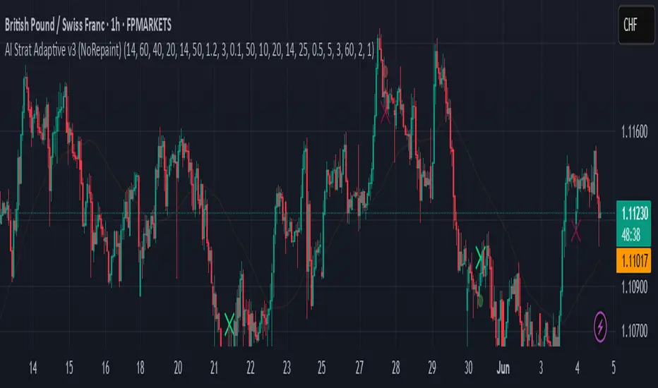
Engulfing Candles with Liquidity SweepOverview
The Engulfing Candles with Liquidity Sweep indicator is designed to highlight high- and low-probability engulfing candle patterns, incorporating liquidity sweep logic for enhanced price action analysis. This script visually marks bullish and bearish engulfing events, differentiating between high-probability and low-probability setups, and plots key Fibonacci levels for each event.
🔶 USAGE
This indicator is ideal for traders seeking to identify potential reversal or continuation points based on engulfing candle patterns and liquidity sweeps. High-probability signals are based on strict engulfing and sweep criteria, while low-probability signals offer additional context for nuanced price action.
• High Probability Engulfing:
Highlights strong bullish or bearish engulfing candles that also sweep the previous candle’s high or low, suggesting a significant shift in market sentiment.
• Low Probability Engulfing:
Marks less strict engulfing patterns where the close remains within the previous candle’s range, providing early signals for potential reversals.
• Fibonacci Levels:
For each detected pattern, the script draws a 50% Fibonacci retracement line, helping traders identify potential retracement or reaction zones.
🔹 SETTINGS
• High Probability Engulfing Settings:
• Customizable colors, line styles, and widths for bullish and bearish fib lines
• Option to show/hide fib lines and pattern markers
• Low Probability Engulfing Settings:
• Separate color and style controls for low-probability signals
• Option to show/hide fib lines and pattern markers
• Alerts:
• Built-in alert conditions for all pattern types, enabling automated notifications
🔶 DETAILS
High Probability Bullish Engulfing:
• Previous candle bearish
• Current candle bullish
• Current low sweeps previous low
• Current close above previous high
High Probability Bearish Engulfing:
• Previous candle bullish
• Current candle bearish
• Current high sweeps previous high
• Current close below previous low
Low Probability Bullish Engulfing:
• Previous candle bearish
• Current candle bullish
• Current low sweeps previous low
• Current close between previous open and high
Low Probability Bearish Engulfing:
• Previous candle bullish
• Current candle bearish
• Current high sweeps previous high
• Current close between previous open and low
🔶 NOTES
• The indicator is fully customizable and can be adapted to various trading styles.
• All signals and levels are plotted directly on the chart for easy reference.
• Alerts can be set for any pattern, supporting both discretionary and automated trading approaches.
Disclaimer:This script is for informational and educational purposes only. It does not constitute financial advice. Use at your own risk.

ICT Killzones Bias & Volume Sweeps @MaxMaserati📌 Overview
This indicator helps traders identify key ICT Killzones (Asian, London, NY AM, NY PM sessions) along with volume analysis and sweep detection. It highlights institutional order blocks, tracks session bias, and detects liquidity sweeps with volume confirmation.
Key Features:
✅ ICT Killzones (Asian, London, NY AM, NY PM)
✅ Volume Analysis (High/Low volume detection)
✅ Sweep Detection (Buyside/Sellside sweeps with volume confirmation)
✅ Session Bias (Bullish/Bearish bias based on price action)
✅ Customizable Sessions (Add personal trading hours)
✅ Institutional Order Build-up (30-min pre-session accumulation zones)
⚙️ Input Settings
1. Timezone Settings
Chart Timezone: Adjust to your local timezone (default: New York).
2. Session Toggles
Asian / London / NY AM / NY PM Sessions: Enable/disable each session.
NY Lunch Session: Optional session (disabled by default).
Personal Trading Time: Customize your trading hours.
3. Label Settings
Label Size: Tiny, Small, Normal, Large.
Session Labels: Customize text for High (H), Low (L), Mid (M) labels.
Background Transparency: Adjust session box opacity.
4. Volume Analysis
Show Volume Labels: Displays volume strength (🚀 Very High, 🔥 High, ⚖️ Normal, 💤 Low, 🐢 Very Low).
Volume Lookback Period: Adjusts volume comparison window.
High/Low Volume Thresholds: Define what constitutes high/low volume.
5. Sweep Detection
Buyside/Sellside Sweeps: Highlights liquidity sweeps.
Sweep Margin: Adjust sensitivity for sweep detection.
Fake Sweep Zones: Option to hide or highlight fakeouts.
Example of Session Sweep and Volume:
Here we have a Bullish Sweep of London Low session by NY AM
However, the volume was low suggesting buyers are not strong enough (M1)
And then the sellers took over and a pressure retest by the buyers of the level and then sellers entered with more power/pressure
6. Session Momentum & Bias
Show Session Bias: Indicates bullish/bearish bias for each session.
Bias Strength Threshold: Adjust sensitivity for bias detection.
📊 How It Works
1. Session Highs/Lows
The indicator tracks High, Low, and Mid prices for each session.
Lines and boxes are drawn to visualize the session range.
2. Volume Analysis
Compares current volume to historical average.
Displays volume strength with emojis (🚀, 🔥, ⚖️, 💤, 🐢).
Highlights high-volume sweeps for confirmation.
3. Sweep Detection
Detects buyside sweeps (liquidity above highs) and sellside sweeps (liquidity below lows).
Sweep zones expand if price lingers near the swept level.
4. 30 minute Pre-session Institutional order buildup
Highlights 30-minute pre-session zones where institutions may accumulate orders.
5. Session Bias
Calculates bias based on open/close price action within the session.
Displays Bullish, Bearish, or Neutral labels.
]
🎯 Trading Applications
1. Liquidity Sweeps
Look for sweeps with high volume as confirmation of institutional activity.
Fade fake sweeps (if enabled) when price reverses quickly.
2. Session Breakouts
Trade breakouts from Asian/London ranges during NY sessions.
Watch for volume expansion on breakouts for confirmation.
3. Pre- Session Institutional Block
Price often reacts to pre-session institutional position build-up (30-min before session opens).
LV:Low Volume, HV: High volume and MV: Medium Volume
NY AM Pre-Session institutional Order Build-up block with high sweep
🔧 Customization Tips
Adjust session times to normal future sessions to match your trading style.
Modify sweep sensitivity if too many/too few sweeps are detected.
Use volume thresholds to fine-tune high/low volume alerts.
📌 Final Notes
This indicator combines ICT concepts with volume analysis for a powerful trading edge. Use it alongside price action and market structure for best results at your own risk.
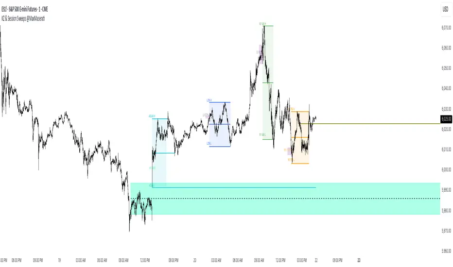
beanBean's Multi-Instrument Pattern Scanner.
This indicator scans H1 timeframe for specific technical patterns. Here's how each pattern is detected:
PATTERN DETECTION CRITERIA:
1. Hammer
- Body Size: ≤ 30% of total candle length
- Lower Wick: > 50% of total candle length
- Upper Wick: < 20% of total candle length
- Formula:
* bodySize = |close - open|
* upperWick = high - max(open, close)
* lowerWick = min(open, close) - low
* totalLength = high - low
2. Shooting Star
- Body Size: ≤ 30% of total candle length
- Upper Wick: > 50% of total candle length
- Lower Wick: < 20% of total candle length
- Uses same measurements as Hammer but inverted
3. Outside/Inside (OI)
Checks three consecutive bars:
- Outside Bar: Bar2 high ≥ Bar3 high AND Bar2 low ≤ Bar3 low
- Inside Bar: Bar1 high ≤ Bar2 high AND Bar1 low ≥ Bar2 low
Pattern confirms when both conditions are met
4. Bullish/Bearish Umbrella
Checks two consecutive bars:
Bullish:
- Current bar's high ≤ previous bar's high
- Current body high ≤ previous bar's high
- Current body low ≥ previous body high
Bearish:
- Current bar's low ≥ previous bar's low
- Current body low ≥ previous bar's low
- Current body high ≤ previous body low
5. Three Bar Triangle (3BT)
Checks three consecutive bars:
- Current bar's high ≤ max(previous two highs)
- Current bar's low ≥ min(previous two lows)
- Indicates price compression
DISPLAY AND ALERTS:
- Patterns are displayed in real-time in the table
- Multiple patterns can be detected simultaneously
- Pattern detection resets each new H1 candle
CONFIGURATION:
- Each row can be independently configured
- Patterns are checked on H1 timeframe close
- Alert frequency: Once per H1 bar close
Note: All measurements use standard OHLC values from only completed H1 candles.
TrendPredator ESThe TrendPredator Essential (ES)
Stacey Burke, a seasoned trader and mentor, developed his trading system over the years, drawing insights from influential figures such as George Douglas Taylor, Tony Crabel, Steve Mauro, and Robert Schabacker. His popular system integrates select concepts from these experts into a consistent framework. While powerful, it is highly discretionary, requiring significant real-time analysis, which can be challenging for novice traders.
The TrendPredator ES indicator supports this approach by automating the essential analysis required to trade the system effectively and incorporating a mechanical bias and multi-timeframe concept.
It provides value to traders by significantly reducing the time needed for session preparation and offering relevant chart analysis and signals for live trading through real-time updates and a unique consolidated table format.
The Stacey Burke Master Pattern
Inspired by Taylor’s 3-day cycle and Steve Mauro’s work with “Beat the Market Maker,” Burke’s system views markets as cyclical, driven by the manipulative patterns of market makers. These patterns often trap traders at the extremes of moves above or below significant levels with peak formations, then reverse to utilize their liquidity, initiating the next phase. Breakouts away from these traps often lead to range expansions, as described by Tony Crabel and Robert Schabacker. After multiple consecutive breakouts, especially after the psychological number three, overextension might develop. A break in structure may then lead to reversals or pullbacks. Burke’s system is designed to track these cycles on the daily timeframe and provides signals and trade setups to navigate along them.
Bias Logic and Multi-Timeframe Concept
The indicator covers the basic signals of his system:
- First Red Day (FRD): Bearish break in structure, signalling weak longs in the market.
- First Green Day (FGD): Bullish break in structure signalling weak shorts in the markt.
- Three Days of Longs (3DL): Overextension signalling potential weak longs in the market.
- Three Days of Shorts (3DS): Overextension signalling potential weak shorts in the market.
- Inside Day (ID): Contraction, signalling potential impulsive reversal or range expansion move.
It enhances the original system by introducing:
Structured Bias Logic:
Tracks bias by following how price trades concerning the last previous candle high or low that was hit. For example if the high was hit, we are bullish above and bearish below.
- Bullish state: Breakout (BO), Fakeout Low (FOL)
- Bearish state: Breakdown (BD), Fakeout High (FOH)
Multi-Timeframe Perspective:
- Tracks all signals across H4, H8, D, W, and M timeframes, to look for alignment and follow trends and momentum in a mechanical way.
The indicator monitors the bias and signals of the system across all relevant timeframes and automates the related graphical chart analysis to generate the information needed for the trader to identify key setups. Additional to the SB pattern, the system helps to identify the higher timeframe situation and follow the moves driven by other timeframe traders.
Example: Full Bullish Cycle on the Daily Timeframe with Signals
- The Trap/Peak Formation
The market breaks down from a previous day’s and maybe week’s low—potentially after multiple breakdowns—but fails to move lower and pulls back up to form a peak formation low and closes as a first green day.
Signal: Bullish daily and weekly fakeout low; three consecutive breakdown days (1W Curr FOL, 1D Curr FOL, BO 3S).
- Pullback and Consolidation
The next day pulls further up after first green day signal, potentially consolidates inside the previous day’s range.
Signal: Fakeout low and first green day closing as an inside day (1D Curr IS, Prev FOL, First G).
- Range Expansion/Trend
The following day breaks up through the previous day’s high, launching a range expansion away from the trap.
Signal: Bullish daily breakout of an inside day (1D Curr BO, Prev IS).
- Overextension
After multiple consecutive breakouts, the market reaches a state of overextension, signalling a possible reversal or pullback.
Signal: Three days of breakout longs (1D Curr BO, Prev BO, BO 3L).
Note: This is only one possible scenario; there are many variations and combinations.
Example Chart: Full Bullish Cycle with Correlated Signals
Note: The signals shown along the move are manually added illustrations. The indicator shows these in realtime in the table at the bottom right. This is only one possible scenario; there are many variations and combinations.
Due to the fractal nature of markets, this cycle can be observed across timeframes. The strongest setups show multi-timeframe alignment. For example, a peak formation and potential reversal on the daily timeframe has high probability and follow-through if it also aligns with bearish signals on higher timeframes (e.g., weekly/monthly BD/FOH) and confirmation on lower timeframes (H4/H8 FOH/BD). With this perspective the system enables the trader to follow the trend and momentum and identify rollover points in a very differentiated way.
Detailed Features and Options
1. Historic Highs and Lows
Displays historic highs and lows per timeframe for added context, enabling users to track sequences over time.
Timeframes: H4, H8, D, W, M
Options: Customize for timeframes shown, number of historic candles per timeframe, colors, formats, and labels.
2. Previous High and Low Extensions
Displays extended previous levels (high, low, and close) for each timeframe to assess how price trades relative to these levels.
H4: P4H, P4L, P4C
H8: P8H, P8L, P8C
Daily: PDH, PDL, PDC
Weekly: PWH, PWL, PWC
Monthly: PMH, PML, PMC
Options: Fully customizable for timeframes shown, colors, formats, and labels.
3. Breach Lines
Tracks live market reactions (e.g., breakouts or fakeouts) per timeframe for the last previous high or low that was hit, highlighting these levels originating at the breached candle to indicate bias (color-coded).
Red: Bearish below
Green: Bullish above
H4: 4FOL, 4FOH, 4BO, 4BD
H8: 8FOL, 8FOH, 8BO, 8BD
D: dFOL, dFOH, dBO, dBD
W: wFOL, wFOH, wBO, wBD
M: mFOL, mFOH, mBO, mBD
Options: Fully customizable for timeframes shown, colors, formats, and labels.
4. Multi-Timeframe Table
Provides a real-time view of system signals, including:
Current Timeframe (Curr): Bias states.
- Breakout (green BO): Bullish after breaking above the previous high.
- Fakeout High (red FOH): Bearish after breaking above the previous high but pulling back down.
- Breakdown (red BD): Bearish after breaking below the previous low.
- Fakeout Low (green FOL): Bullish after breaking below the previous low but pulling back up.
- Inside (IS): Price trading neutral inside the previous range, taking the previous bias (color indicates the previous bias).
Previous Timeframe (Prev): Tracks last candle bias state and transitions dynamically.
- Bias for last candle: BO, FOH, BD, FOL in respective colors.
- Inside bar (yellow IS): Indicated as standalone signal.
Note: Also previous timeframes get constantly updated in real time to track the bias state in relation to the level that was hit. This means a BO can still lose the level and become a FOH, and vice versa, and a BD can still become a FOL, and vice versa. This is critical to see for example if traders that are trapped in that timeframe with a FOH or FOL are released. An inside bar stays fixed, though, since no level was hit in that timeframe.
Breakouts (BO): Breakout count 3 longs and 3 shorts.
- 3 Longs (red 3L): Bearish after three breakouts without hitting a previous low.
- 3 Shorts (green 3S): Bullish after three breakdowns without hitting a previous high.
First Countertrend Close (First): Tracks First Red or Green Day.
- First Green (G): After two consecutive red closes.
- First Red (R): After two consecutive green closes.
Options: Customizable font size and label colors.
Overall Options:
Toggle single feature groups on/off.
Customize H8 open/close time as an offset to UTC to be provider independent.
Colour settings for dark or bright backgrounds.
Using the Indicator for Trading
The automated analysis provided by the indicator can be used for thesis generation in preparation for a session as well as for live trading, leveraging the real-time updates. It is recommended to customize the settings accordingly, such as hiding the lower timeframes for thesis generation to keep the charts clean.
1. Setup Identification:
Follow the bias of daily and H8 timeframes. A setup always requires alignment of these.
Setup Types:
- Trend Trade: Trade in alignment with the previous day’s trend.
Example: Price above the previous day’s high → Focus on long setups (dBO, H8 FOL) until overextension or reversal signs appear (H8 BO 3L, First R).
- Reversal Trade: Identify reversal setups when lower timeframes show rollovers after higher timeframe weakness.
Example: Price below the previous day’s high after FOH → Look for reversal signals at the current high of day (H8 FOH, BO 3L, First R).
2. Context Assessment:
Evaluate alignment of higher timeframes (e.g., Month/Week, Week/Day). More alignment → Stronger setups. Conflicting situations → Setups invalidated.
3. Entry Confirmation:
Confirm entries based on H8 and H4 alignment and candle closes (e.g., M15 or M5 close after entering setup zone as confirmation).
Example Chart for Reversal Trade:
1. Setup Identification: FOH continuation after BO 3L overextension, confirmed by H8 FOH, First R.
2. Context Assessment: Month in FOL with bearish First R; Week in BO but bearishly overextended with BO 3L.
3. Entry Confirmation: H4 BD, M5 close.
Further recommendations:
- Higher timeframe context: TPO or volume profile indicators can be used to gain an even better overview.
- Entry confirmation: Momentum indicators like VWAP, Supertrend, or EMA are helpful for increasing precision. Additionally, tracking lower timeframe fakeouts can provide powerful confluence.
- Late session trading: Entries later in the session, such as during the 3rd hour of the NY session, offer better analysis and follow-through on setups.
Limitations:
Data availability using TradingView has its limitations. The indicator leverages only the real-time data available for the specific timeframe being used. This means it cannot access data from timeframes lower than the one displayed on the chart. For example, if you are on a daily chart, it cannot use H8 data. Additionally, on very low timeframes, the historical availability of data might be limited, making higher timeframe signals unreliable.
To address this, the indicator automatically hides the affected columns in these specific situations, preventing false signals.
Disclaimer
This indicator is for educational purposes only and does not guarantee profits.
None of the information provided shall be considered financial advice.
The indicator does not provide final buy or sell signals but highlights zones for potential setups.
Users are fully responsible for their trading decisions and outcomes.

Daily Weekly Monthly Highs & Lows - Alerts !
1. Purpose
The script helps traders:
• Visualize the high and low levels for the previous daily, weekly, and monthly periods.
• Receive alerts when the current price crosses these levels.
• Identify key support and resistance zones based on historical highs and lows.
2. Key Features
User Inputs
The script offers customization options through input parameters:
• Daily Levels:
• Enable/disable displaying daily levels (Show Daily Levels).
• Customize the color for daily level lines (Daily Line Color).
• Weekly Levels:
• Enable/disable displaying weekly levels (Show Weekly Levels).
• Customize the color for weekly level lines (Weekly Line Color).
• Monthly Levels:
• Enable/disable displaying monthly levels (Show Monthly Levels).
• Customize the color for monthly level lines (Monthly Line Color).
3. Core Functionality
Level Calculations
The script retrieves the previous daily, weekly, and monthly highs and lows using the request.security() function:
• Daily High/Low: Taken from the previous day’s high and low.
• Weekly High/Low: Taken from the previous week’s high and low.
• Monthly High/Low: Taken from the previous month’s high and low.
Price Crossing Detection
For each level (daily, weekly, monthly), the script checks if the current high or low price has crossed:
• The previous high (triggering a “High Reached” alert).
• The previous low (triggering a “Low Reached” alert).
4. Visual Features
The script plots lines to represent the previous highs and lows:
• Daily Levels:
• Dashed lines for the previous daily high and low.
• Configurable color (Daily Line Color).
• Weekly Levels:
• Dashed lines for the previous weekly high and low.
• Configurable color (Weekly Line Color).
• Monthly Levels:
• Dashed lines for the previous monthly high and low.
• Configurable color (Monthly Line Color).
These lines extend forward by one bar for better visibility on the chart.
5. Alert Features
The script provides alerts for when the price crosses these levels:
• Daily Alerts:
• “Daily High Reached” when the current price crosses the previous daily high.
• “Daily Low Reached” when the current price crosses the previous daily low.
• Weekly Alerts:
• “Weekly High Reached” when the current price crosses the previous weekly high.
• “Weekly Low Reached” when the current price crosses the previous weekly low.
• Monthly Alerts:
• “Monthly High Reached” when the current price crosses the previous monthly high.
• “Monthly Low Reached” when the current price crosses the previous monthly low.
6. Practical Use Case
This script is ideal for traders who:
• Use support and resistance levels from daily, weekly, and monthly timeframes as part of their strategy.
• Want to monitor price interactions with these levels in real-time.
• Need automatic alerts for key price movements without continuously monitoring the chart.
7. Limitations
• Max Line Count: TradingView limits the number of lines that can be drawn on the chart to max_lines_count = 500.
• No Historical Levels: The script only tracks the most recent daily, weekly, and monthly levels and does not display historical levels.
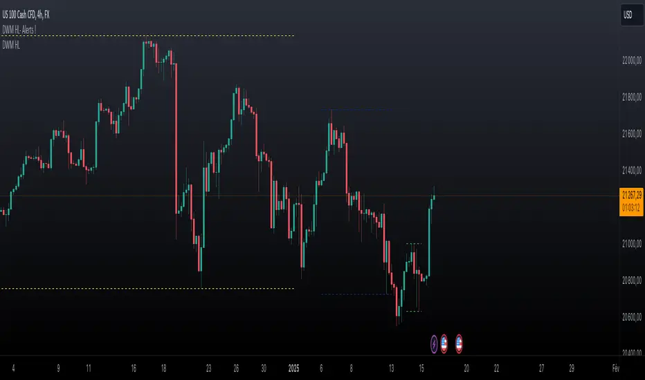
ICTProTools | ICT Insight - Time & Price Zones🚀 INTRODUCTION
The Time and Price Zones indicator builds upon the foundational concepts of ICT (Inner Circle Trader) and Smart Money Concepts (SMC). These methodologies analyze the behavior of institutional traders (known as "smart money") by focusing on liquidity, key price levels, and market timing.
Liquidity refers to areas with high concentrations of pending orders (stops, take-profits, entries) in the market. Large institutions efficiently need to execute their massive orders without causing excessive slippage. To achieve this, they strategically create and exploit liquidity pools by driving the price toward areas where retail traders cluster their positions.
Then, through "liquidity grabs" or "stop hunts,” institutions accumulate or distribute positions at optimal prices . This strategy allows them to fill large orders with minimal market impact, typically clearing out retail traders' positions before the price reverses.
This indicator helps traders apply these principles by merging time-based and price-based analysis tools for better market understanding. By combining high-impact sessions like Kill Zones with pivotal price markers such as Previous Highs and Lows, traders can see where institutional activity intersects with liquidity pools, improving their decision-making.
This powerful combination allows users to monitor market dynamics in real time, helping them spot sentiment shifts and identify crucial turning points more effectively.
💎 FEATURES
Kill Zones
Kill Zones are critical periods of the trading day characterized by heightened institutional activity, resulting in increased liquidity and significant price movements. By recognizing these zones, you can strategically focus your efforts on the most advantageous moments for trading.
The Asian Session , which runs from 5 PM to 1 AM New York time, serves as an essential liquidity provider before the onset of more volatile trading periods. This session is intricately linked to the Smart Money Tool (SMT - See below), as the highs and lows established during this period provide foundational liquidity levels. You can set alerts when these levels are breached , allowing you to stay informed without constant chart monitoring and make timely trading decisions.
Transitioning into the London Kill Zone from 2 to 5 AM New York time marks the beginning of the European session, often associated with increased volatility. Following this, the New York Kill Zone , occurring from 7 to 10 AM , sees significant overlap between the London and New York sessions, where liquidity flows intensify and frequently correlate with notable price reversals. Finally, the London Close from 10 to 12 PM signifies the end of the European session, often ending the day with a retracement in the daily range.
Thanks to the timezone you can select relative to a region, Kill Zones will automatically adapt to time changes throughout the year and between different brokers , ensuring accurate Kill Zone timings without manual adjustments.
Incorporating our advanced Kill Zones indicator into your trading strategy gives you unparalleled insights and enhanced functionality. With integrated alerts for breaches of key levels, you can stay informed and ready to act without the need for constant chart monitoring, allowing you to focus on executing your trading strategies effectively.
We can see on this chart the identified Kill Zones during the trading day on EURUSD , including the Asian Session in gray, which tends to consolidate slightly (creating liquidity), the London Kill Zone in orange, which tends to move fast, often taking Asian quickly, the New York Kill Zone in green, with always a lot of movements, and the London Close in blue, seeming rather to retrace.
The midline indicates the 50% mark of the session, serving as a reference point for potential price reactions. Additionally, the highs and lows established during the Asian Session are linked to the Smart Money Tool (SMT) and can trigger alerts when breached. Here, you could have received an alert when Asian Low (marked AL) and Asian High (marked AH) were swept.
Previous & Open Levels
Previous and Open levels are key elements in ICT methodology, showing important price points from major timeframes (Daily, Weekly, Monthly). These levels (Previous High, Low, Open, and their separators) help traders understand price dynamics and anticipate market shifts.
The Previous levels connect directly to the Smart Money Tool (SMT - See below) as they provide foundational liquidity levels. In ICT methodology, previous are levels where many traders place their Stop Loss, thus creating liquidity. This helps you understand potential market reactions and whether prices will likely continue their trend or reverse.
You’ll be instantly notified whenever the price interacts with any of these Previous levels. This means you can stay informed about critical market movements without the need to monitor your charts constantly.
The indicator also displays Opening prices and includes separators for daily, weekly, and monthly levels, offering a clear market overview.
Open levels can act as simplified indicators of Premium and Discount Zones. To be above the opening price can be considered as the Premium Zone , where the market offers higher prices, typically suitable for selling opportunities. Conversely, to be below this price can be considered as the Discount Zone , where prices are relatively lower, offering potential buying opportunities.
These visual elements help you identify crucial market zones that reflect both past price action and current market dynamics.
Our indicator offers you the exclusive ability to integrate the True Day Range, as described by ICT. Based on institutional logic, this concept defines the trading day starting at 00:00 New York time. You can adapt this flexible feature to match your trading style and analysis needs.
By incorporating our advanced Previous levels indicator into your trading arsenal, you gain powerful insights and enhanced functionality.
The chart above displays key Previous and open levels on EURUSD , including the Month, Week, and Day lines, along with separators for enhanced clarity. All levels are based on the True Day Range Mode. The notes indicate significant price points, highlighting how the price interacts with these important levels, which helps us to understand it…
We can start with the biggest liquidity, the Previous Month. In this example, we can see the PMH, and the price seems to have used this level as a reversal point. The PM levels are indeed significant liquidity zones. We can observe the creation of wicks that interact with this level, signaling a liquidity grab.
Following this, the price drops quickly before rebounding, creating a liquidity range, that will probably be liquidated then… This is why it rises again to form what is now the PDH (Previous Day High), using it as liquidity (inducement) while using the PWH (Previous Week High) as a rebound level. The PWH is indeed a High Resistance (HR) area since there is only a few liquidity at this point thanks to the liquidity grab. The price has no reason to move higher.
Looking ahead, we can forecast that the price may continue its decline, potentially targeting lower liquidity levels. There is likely additional liquidity beneath the current range, particularly near the PDL (Previous Day Low) and PWL (Previous Week Low).
Additionally, we can note that at this point, the price was above the D.O.P (Daily Open) and W.O.P (Weekly Open), areas where selling would be more favorable. The price reacts significantly around these levels, creating large wicks, demonstrating their importance.
SMT Dashboard (Smart Money Tool)
The Smart Money Tool (SMT) is a powerful concept within the ICT methodology that enables you to compare various assets based on liquidity uptake from significant price levels.
By utilizing the SMT, you can analyze any asset , whether it’s a currency pair, stock, cryptocurrency, or other financial instruments. The dashboard helps you identify the strongest and weakest assets by analyzing their interactions with critical liquidity levels and identifying divergences , including those related to the Previous Month, Previous Week, Previous Day, and Asian Session Highs and Lows. By doing so, he identifies the most bullish symbol. It will therefore tend to rise more easily, or at least fall less, than the other one.
The SMT includes alert functionality that notifies you whenever a new SMT is created or has changed , allowing you to stay informed about which asset is currently the strongest. This means you can react promptly to market changes without constantly monitoring your charts.
Additionally, since the SMT relies on the Previous levels, it is influenced by the selected mode, whether based on traditional Previous levels or the True Day Range . This flexibility ensures that you are using the most relevant information available for your trading decisions. Asian High and Asian Low levels are also calculated according to the schedules configured in the Kill Zones section.
In summary, the Smart Money Tool displays the strongest and weakest assets based on liquidity uptake, providing you with clear information on which asset to prioritize, so you can maximize your potential profits. By incorporating this concept into your approach, you align your decisions with prevailing market dynamics, offering you unparalleled insights and features tailored to enhance your trading strategy.
This chart displays the Smart Money Tool (SMT) dashboard on the GBPUSD symbol, which compares the liquidity uptake for EURUSD and GBPUSD pairs. The indicator shows that both Previous Month's and Week's High and Low were taken for both pairs. However, the Asian High (AH) has been breached on GBPUSD but not on EURUSD, while the Asian Low (AL) has been taken by EURUSD. As a result, GBPUSD is identified as the stronger asset, indicating that traders should focus on buying opportunities with GBPUSD rather than EURUSD. This analysis helps traders prioritize the best symbol for their strategies based on the most relevant liquidity divergences.
✨ SETTINGS
Kill Zones: Customize the display options for the Asian (with lines), London, New York, and London Close Kill Zones. Configure timezone options, midlines, and color preferences.
Previous & Open Levels: Adjust how Previous High/Low levels, Open and separators are displayed. Select between Classic or True Day Range Mode based on your trading preferences.
SMT: Choose the correlated assets for the SMT comparison and select which liquidity (Monthly, Weekly, Daily, Asian) to use and display. Configure settings like liquidity sweeps and strongest pair emojis.
Alerts: Configure alerts for key events such as the Asian High/Low or Previous Levels liquidity sweep, and SMT divergences.
🎯 CONCLUSION
The Time and Price Zones indicator offers a practical and insightful approach to market analysis by combining major principles of ICT and Smart Money Concepts into a cohesive tool. It empowers traders to understand key price levels, liquidity dynamics, and institutional activity with ease. By helping traders avoid being the liquidity of the market and instead align with institutional flows, the indicator can significantly enhance performances. While its features provide a valuable edge, it’s essential to remember that none should be used on its own and many more factors go into being a profitable trader.

Inner Bar Strength (IBS)Inner Bar Strength (IBS) Indicator
The Inner Bar Strength (IBS) indicator is a technical analysis tool designed to measure the position of the closing price relative to the day's price range. It provides insights into market sentiment by indicating where the close occurs within the high and low of a specific timeframe. The IBS value ranges from 0 to 1, where values near 1 suggest bullish momentum (close near the high), and values near 0 indicate bearish momentum (close near the low).
How It Works
The IBS is calculated using the following formula:
IBS = (Close−Low) / (High−Low)
IBS = (High−Low) / (Close−Low)
Close: Closing price of the selected timeframe.
Low: Lowest price of the selected timeframe.
High: Highest price of the selected timeframe.
The indicator allows you to select the timeframe for calculation (default is daily), providing flexibility to analyze different periods based on your trading strategy.
Key Features
Inner Bar Strength (IBS) Indicator
The Inner Bar Strength (IBS) indicator is a technical analysis tool designed to measure the position of the closing price relative to the day's price range. It provides insights into market sentiment by indicating where the close occurs within the high and low of a specific timeframe. The IBS value ranges from 0 to 1, where values near 1 suggest bullish momentum (close near the high), and values near 0 indicate bearish momentum (close near the low).
How It Works
The IBS is calculated using the following formula:
IBS=Close−LowHigh−Low
IBS=High−LowClose−Low
Close: Closing price of the selected timeframe.
Low: Lowest price of the selected timeframe.
High: Highest price of the selected timeframe.
The indicator allows you to select the timeframe for calculation (default is daily), providing flexibility to analyze different periods based on your trading strategy.
Key Features
Timeframe Selection: Customize the timeframe to daily, weekly, monthly, or any other period that suits your analysis.
Adjustable Thresholds: Input fields for upper and lower thresholds (defaulted at 0.9 and 0.1) help identify overbought and oversold conditions.
Visual Aids: Dashed horizontal lines at the threshold levels make it easy to visualize critical levels on the chart.
How to Use the IBS Indicator
When the IBS value exceeds the upper threshold (e.g., 0.9), it suggests the asset is closing near its high and may be overbought.
When the IBS value falls below the lower threshold (e.g., 0.1), it indicates the asset is closing near its low and may be oversold.
Use RSI to confirm overbought or oversold conditions identified by the IBS.
Incorporate moving averages to identify the overall trend and filter signals.
High trading volume can strengthen signals provided by the IBS.
If the price is making lower lows while the IBS is making higher lows, it may signal a potential upward reversal.
If the price is making higher highs and the IBS is making lower highs, a downward reversal might be imminent.
Conclusion
The Inner Bar Strength (IBS) indicator is a valuable tool for traders seeking to understand intraday momentum and potential reversal points. By measuring where the closing price lies within the day's range, it provides immediate insights into market sentiment. When used alongside other technical analysis tools, the IBS can enhance your trading strategy by identifying overbought or oversold conditions, confirming breakouts, and highlighting potential divergence signals.

Exposure Oscillator (Cumulative 0 to ±100%)
Exposure Oscillator (Cumulative 0 to ±100%)
This Pine Script indicator plots an "Exposure Oscillator" on the chart, which tracks the cumulative market exposure from a range of technical buy and sell signals. The exposure is measured on a scale from -100% (maximum short exposure) to +100% (maximum long exposure), helping traders assess the strength of their position in the market. It provides an intuitive visual cue to aid decision-making for trend-following strategies.
Buy Signals (Increase Exposure Score by +10%)
Buy Signal 1 (Cross Above 21 EMA):
This signal is triggered when the price crosses above the 21-period Exponential Moving Average (EMA), where the current bar closes above the EMA21, and the previous bar closed below the EMA21. This indicates a potential upward price movement as the market shifts into a bullish trend.
buySignal1 = ta.crossover(close, ema21)
Buy Signal 2 (Trending Above 21 EMA):
This signal is triggered when the price closes above the 21-period EMA for each of the last 5 bars, indicating a sustained bullish trend. It confirms that the price is consistently above the EMA21 for a significant period.
buySignal2 = ta.barssince(close <= ema21) > 5
Buy Signal 3 (Living Above 21 EMA):
This signal is triggered when the price has closed above the 21-period EMA for each of the last 15 bars, demonstrating a strong, prolonged uptrend.
buySignal3 = ta.barssince(close <= ema21) > 15
Buy Signal 4 (Cross Above 50 SMA):
This signal is triggered when the price crosses above the 50-period Simple Moving Average (SMA), where the current bar closes above the 50 SMA, and the previous bar closed below it. It indicates a shift toward bullish momentum.
buySignal4 = ta.crossover(close, sma50)
Buy Signal 5 (Cross Above 200 SMA):
This signal is triggered when the price crosses above the 200-period Simple Moving Average (SMA), where the current bar closes above the 200 SMA, and the previous bar closed below it. This suggests a long-term bullish trend.
buySignal5 = ta.crossover(close, sma200)
Buy Signal 6 (Low Above 50 SMA):
This signal is true when the lowest price of the current bar is above the 50-period SMA, indicating strong bullish pressure as the price maintains itself above the moving average.
buySignal6 = low > sma50
Buy Signal 7 (Accumulation Day):
An accumulation day occurs when the closing price is in the upper half of the daily range (greater than 50%) and the volume is larger than the previous bar's volume, suggesting buying pressure and accumulation.
buySignal7 = (close - low) / (high - low) > 0.5 and volume > volume
Buy Signal 8 (Higher High):
This signal occurs when the current bar’s high exceeds the highest high of the previous 14 bars, indicating a breakout or strong upward momentum.
buySignal8 = high > ta.highest(high, 14)
Buy Signal 9 (Key Reversal Bar):
This signal is generated when the stock opens below the low of the previous bar but rallies to close above the previous bar’s high, signaling a potential reversal from bearish to bullish.
buySignal9 = open < low and close > high
Buy Signal 10 (Distribution Day Fall Off):
This signal is triggered when a distribution day (a day with high volume and a close near the low of the range) "falls off" the rolling 25-bar period, indicating the end of a bearish trend or selling pressure.
buySignal10 = ta.barssince(close < sma50 and close < sma50) > 25
Sell Signals (Decrease Exposure Score by -10%)
Sell Signal 1 (Cross Below 21 EMA):
This signal is triggered when the price crosses below the 21-period Exponential Moving Average (EMA), where the current bar closes below the EMA21, and the previous bar closed above it. It suggests that the market may be shifting from a bullish trend to a bearish trend.
sellSignal1 = ta.crossunder(close, ema21)
Sell Signal 2 (Trending Below 21 EMA):
This signal is triggered when the price closes below the 21-period EMA for each of the last 5 bars, indicating a sustained bearish trend.
sellSignal2 = ta.barssince(close >= ema21) > 5
Sell Signal 3 (Living Below 21 EMA):
This signal is triggered when the price has closed below the 21-period EMA for each of the last 15 bars, suggesting a strong downtrend.
sellSignal3 = ta.barssince(close >= ema21) > 15
Sell Signal 4 (Cross Below 50 SMA):
This signal is triggered when the price crosses below the 50-period Simple Moving Average (SMA), where the current bar closes below the 50 SMA, and the previous bar closed above it. It indicates the start of a bearish trend.
sellSignal4 = ta.crossunder(close, sma50)
Sell Signal 5 (Cross Below 200 SMA):
This signal is triggered when the price crosses below the 200-period Simple Moving Average (SMA), where the current bar closes below the 200 SMA, and the previous bar closed above it. It indicates a long-term bearish trend.
sellSignal5 = ta.crossunder(close, sma200)
Sell Signal 6 (High Below 50 SMA):
This signal is true when the highest price of the current bar is below the 50-period SMA, indicating weak bullishness or a potential bearish reversal.
sellSignal6 = high < sma50
Sell Signal 7 (Distribution Day):
A distribution day is identified when the closing range of a bar is less than 50% and the volume is larger than the previous bar's volume, suggesting that selling pressure is increasing.
sellSignal7 = (close - low) / (high - low) < 0.5 and volume > volume
Sell Signal 8 (Lower Low):
This signal occurs when the current bar's low is less than the lowest low of the previous 14 bars, indicating a breakdown or strong downward momentum.
sellSignal8 = low < ta.lowest(low, 14)
Sell Signal 9 (Downside Reversal Bar):
A downside reversal bar occurs when the stock opens above the previous bar's high but falls to close below the previous bar’s low, signaling a reversal from bullish to bearish.
sellSignal9 = open > high and close < low
Sell Signal 10 (Distribution Cluster):
This signal is triggered when a distribution day occurs three times in the rolling 7-bar period, indicating significant selling pressure.
sellSignal10 = ta.valuewhen((close < low) and volume > volume , 1, 7) >= 3
Theme Mode:
Users can select the theme mode (Auto, Dark, or Light) to match the chart's background or to manually choose a light or dark theme for the oscillator's appearance.
Exposure Score Calculation: The script calculates a cumulative exposure score based on a series of buy and sell signals.
Buy signals increase the exposure score, while sell signals decrease it. Each signal impacts the score by ±10%.
Signal Conditions: The buy and sell signals are derived from multiple conditions, including crossovers with moving averages (EMA21, SMA50, SMA200), trend behavior, and price/volume analysis.
Oscillator Visualization: The exposure score is visualized as a line on the chart, changing color based on whether the exposure is positive (long position) or negative (short position). It is limited to the range of -100% to +100%.
Position Type: The indicator also indicates the position type based on the exposure score, labeling it as "Long," "Short," or "Neutral."
Horizontal Lines: Reference lines at 0%, 100%, and -100% visually mark neutral, increasing long, and increasing short exposure levels.
Exposure Table: A table displays the current exposure level (in percentage) and position type ("Long," "Short," or "Neutral"), updated dynamically based on the oscillator’s value.
Inputs:
Theme Mode: Choose "Auto" to use the default chart theme, or manually select "Dark" or "Light."
Usage:
This oscillator is designed to help traders track market sentiment, gauge exposure levels, and manage risk. It can be used for long-term trend-following strategies or short-term trades based on moving average crossovers and volume analysis.
The oscillator operates in conjunction with the chart’s price action and provides a visual representation of the market’s current trend strength and exposure.
Important Considerations:
Risk Management: While the exposure score provides valuable insight, it should be combined with other risk management tools and analysis for optimal trading decisions.
Signal Sensitivity: The accuracy and effectiveness of the signals depend on market conditions and may require adjustments based on the user’s trading strategy or timeframe.
Disclaimer:
This script is for educational purposes only. Trading involves significant risk, and users should carefully evaluate all market conditions and apply appropriate risk management strategies before using this tool in live trading environments.

Nasan Hull-smoothed envelope The Nasan Hull-Smoothed Envelope indicator is a sophisticated overlay designed to track price movement within an adaptive "envelope." It dynamically adjusts to market volatility and trend strength, using a series of smoothing and volatility-correction techniques. Here's a detailed breakdown of its components, from the input settings to the calculated visual elements:
Inputs
look_back_length (500):
Defines the lookback period for calculating intraday volatility (IDV), smoothing it over time. A higher value means the indicator considers a longer historical range for volatility calculations.
sl (50):
Sets the smoothing length for the Hull Moving Average (HMA). The HMA smooths various lines, creating a balance between sensitivity and stability in trend signals.
mp (1.5):
Multiplier for IDV, scaling the volatility impact on the envelope. A higher multiplier widens the envelope to accommodate higher volatility, while a lower one tightens it.
p (0.625):
Weight factor that determines the balance between extremes (highest high and lowest low) and averages (sma of high and sma of low) in the high/low calculations. A higher p gives more weight to extremes, making the envelope more responsive to abrupt market changes.
Volatility Calculation (IDV)
The Intraday Volatility (IDV) metric represents the average volatility per bar as an exponentially smoothed ratio of the high-low range to the close price. This is calculated over the look_back_length period, providing a base volatility value which is then scaled by mp. The IDV enables the envelope to dynamically widen or narrow with market volatility, making it sensitive to current market conditions.
Composite High and Low Bands
The high and low bands define the upper and lower bounds of the envelope.
High Calculation
a_high:
Uses a multi-period approach to capture the highest highs over several intervals (5, 8, 13, 21, and 34 bars). Averaging these highs provides a more stable reference for the high end of the envelope, capturing both immediate and recent peak values.
b_high:
Computes the average of shorter simple moving averages (5, 8, and 13 bars) of the high prices, smoothing out fluctuations in the recent highs. This generates a balanced view of high price trends.
high_c:
Combines a_high and b_high using the weight p. This blend creates a composite high that balances between recent peaks and smoothed averages, making the upper envelope boundary adaptive to short-term price shifts.
Low Calculation
a_low and b_low:
Similar to the high calculation, these capture extreme lows and smooth low values over the same intervals. This approach creates a stable and adaptive lower bound for the envelope.
low_c:
Combines a_low and b_low using the weight p, resulting in a composite low that adjusts to price fluctuations while maintaining a stable trend line.
Volatility-Adjusted Bands
The final composite high (c_high) and composite low (c_low) bands are adjusted using IDV, which accounts for intraday volatility. When volatility is high, the bands expand; when it’s low, they contract, providing a visual representation of volatility-adjusted price bounds.
Basis Line
The basis line is a Hull Moving Average (HMA) of the average of c_high and c_low. The HMA is known for its smoothness and responsiveness, making the basis line a central trend indicator. The color of the basis line changes:
Green when the basis line is increasing.
Red when the basis line is decreasing.
This color-coded basis line serves as a quick visual reference for trend direction.
Short-Term Trend Strength Block
This component analyzes recent price action to assess short-term bullish and bearish momentum.
Conditions (green, red, green1, red1):
These are binary conditions that categorize price movements as bullish or bearish based on the close compared to the open and the close’s relationship with the exponential moving average (EMA). This separation helps capture different types of strength (above/below EMA) and different bullish or bearish patterns.
Composite Trend Strength Values:
Each of the bullish and bearish counts (above and below the EMA) is normalized, resulting in the following values:
green_EMAup_a and red_EMAup_a for bullish and bearish strength above the EMA.
green_EMAdown_a and red_EMAdown_a for bullish and bearish strength below the EMA.
Trend Strength (t_s):
This calculated metric combines the normalized trend strengths with extra weight to conditions above the EMA, giving more relevance to trends that have momentum behind them.
Enhanced Trend Strength
avg_movement:
Calculates the average absolute price movement over the short_term_length, providing a measurement of recent price activity that scales with volatility.
enhanced_t_s:
Multiplies t_s by avg_movement, creating an enhanced trend strength value that reflects both directional strength and the magnitude of recent price movement.
min and max:
Minimum and maximum percentile thresholds, respectively, based on enhanced_t_s for controlling the color gradient in the fill area.
Fill Area
The fill area between plot_c_high and plot_c_low is color-coded based on the enhanced trend strength (enhanced_t_s):
Gradient color transitions from blue to green based on the strength level, with blue representing weaker trends and green indicating stronger trends.
This visual fill provides an at-a-glance assessment of trend strength across the envelope, with color shifts highlighting momentum shifts.
Summary
The indicator’s purpose is to offer an adaptive price envelope that reflects real-time market volatility and trend strength. Here’s what each component contributes:
Basis Line: A trend-following line in the center that adjusts color based on trend direction.
Envelope (c_high, c_low): Adapts to volatility by expanding and contracting based on IDV, giving traders a responsive view of expected price bounds.
Fill Area: A color-gradient region representing trend strength within the envelope, helping traders easily identify momentum changes.
Overall, this tool helps to identify trend direction, market volatility, and strength of price movements, allowing for more informed decisions based on visual cues around price boundaries and trend momentum.

Market Structure Overlay🚀 Market Structure Overlay Indicator 🚀
🔍 Overview
The Market Structure Overlay (MSO) is a sophisticated technical analysis tool created to analyze price action and understand market structure in a more precise way. It identifies Break of Structure (BOS), Market Structure Breaks (MSBs), Equal Highs (EQH), and Equal Lows (EQL) with meticulous precision by utilizing both wicks and closing prices for better accuracy. The MSO is suitable for all trading timeframes, providing traders with the flexibility to observe and trade on any scale, from intraday to long-term trends.
⚙️ How It Works
The MSO uses advanced logic to detect critical price levels that highlight structural changes in the market. It calculates swing highs and lows using user-defined settings, allowing for customization in market structure analysis. The indicator further highlights BOS and MSB levels by leveraging supply and demand detection, offering a comprehensive understanding of trend reversals and continuation points.
✨ Key features include:
📈 Bullish and Bearish BOS/MSB Lines: MSO differentiates between bullish and bearish structural events, which helps traders understand the prevailing trend and identify key pivot points.
🎨 Customizable Appearance: Traders can personalize line styles and colors for BOS/MSB, trendlines and EQH/EQL, making the tool integrate seamlessly into any chart setup.
🔄 Swing Length and Demand Memory Settings: MSO allows users to specify the swing length for BOS lookback and how many historical zones should be stored on the chart, enhancing control over how much data is analyzed visually.
📊 Market Structure Elements Explained
Break of Structure (BOS): A BOS occurs when the price breaks through a previous Higher High (HH) or Lower Low (LL), indicating a continuation of the current trend. It helps confirm the prevailing market direction.
Market Structure Break (MSB): occurs when a Higher Low (HL) or Lower High (LH) is broken, signaling a potential shift in the market trend. This typically marks the beginning of a trend reversal.
Equal Highs (EQH) and Equal Lows (EQL): These levels are areas of liquidity where previous highs or lows are tested again by the market, often signifying areas of accumulation or distribution. EQH and EQL are crucial for recognizing potential liquidity traps.
Trendlines: Trendlines are used to connect successive highs or lows, providing a visual representation of the current direction of the market. They help traders understand trend momentum and potential breakouts.
🔥 Key Features and Benefits
✅ Accurate Market Structure Detection
The Market Structure Overlay identifies Break of Structure (BOS) and Market Structure Breaks (MSB) events that indicate potential trend changes or continuations. The indicator also distinguishes between bullish and bearish market structures using color-coded lines and custom labels, which helps in immediately identifying market dynamics.
📊 Supply and Demand Zones for BOS/MSB Detection
The MSO uses Supply and Demand Zones as part of the detection logic for BOS and MSB. Although these zones are not directly plotted, they play a key role in determining when a significant structural break occurs. This unique approach enhances the accuracy of BOS and MSB identification, as it takes into account areas of accumulation or distribution that often serve as precursors to trend shifts.
🔍 Equal Highs and Lows Detection
The MSO features Equal Highs (EQH) and Equal Lows (EQL) detection, which is a significant indicator for liquidity zones where potential orders might be resting. These areas often trigger key price actions as they get tested or broken.
⚙️ Customizable Settings
Users can customize the indicator’s behavior, including choosing whether to use candle wicks or closing prices, setting swing lengths for identifying key levels, and specifying memory for storing past zones. This flexibility allows traders to adjust the indicator to suit their personal trading strategy and preferences.
⏱️ Multi-Timeframe Highs and Lows
The indicator includes multi-timeframe support for significant highs and lows (daily, weekly, monthly, yearly). This helps traders understand where they are in the larger market context, especially when making decisions during intra-session trading.
🔎 Precise Detection Approach
Unlike traditional market structure indicators that rely heavily on simple pivot points, the MSO employs a more advanced and precise detection mechanism for BOS and MSB. Traditional pivot points typically use a lookback function to identify highs and lows over a fixed period, which can lead to false signals due to market noise or temporary price fluctuations. In contrast, the MSO records and checks swing and interim points against stored memory, only signaling structural breaks after a thorough evaluation. This results in a non-repainting and highly accurate depiction of market structure, minimizing false alerts and providing traders with reliable insights based on price action that remains consistent once confirmed.
🎨 Visualization Options
The MSO uses color-coded BOS and MSB lines to easily differentiate between bullish and bearish scenarios. Users also have options to visualize equal highs/lows (EQH/EQL) to recognize potential liquidity points. A detailed breakdown of Supply and Demand Zones helps traders identify high-probability areas for entries and exits. Additionally, the indicator allows traders to toggle visibility of key elements, including trend lines, labels, and multi-timeframe levels.
📝 Summary
The Market Structure Overlay is an essential tool for understanding price behavior and structural shifts in any financial market. Its use of sophisticated logic to detect structural breaks, coupled with customizable visualizations, allows traders to gain a nuanced view of market dynamics. The supply and demand zones, together with the BOS, MSB, EQH, and EQL labels, provide a strong foundation for both trend-following and reversal trading strategies.
MSO is not just a tool for understanding market direction—it's designed to enhance decision-making by delivering reliable and actionable insights into market structure. This indicator provides a seamless blend of market theory with advanced technical features, making it a valuable asset for serious traders.
📊 Key Visual Examples:
📈 Bullish and Bearish BOS/MSB Lines
📸
🌀 Trendlines
📸
⚠️ Note:
This indicator should be used as part of a broader trading strategy. Always confirm your entries and exits with additional tools and analysis methods. 💡

Key Levels Suite - By LeviathanThis is a comprehensive script, designed to display over 100 key price levels across multiple dimensions, including volume profile levels, HTF levels, VWAPs, SMAs/EMAs, market session levels, day of week levels and more. The indicator offers high flexibility in features, settings and visual appearance.
● The script organizes levels into six main categories:
Higher Timeframe (HTF) Levels
- Current and/or previous period: Open, High, Low, and Midpoint for Daily, Weekly, Monthly, Quarterly, and Yearly timeframes (eg. levels for current weekly high/low and previous weekly high/low).
- These levels provide a clear structure for identifying key support and resistance zones. Traders often use HTF levels to anticipate price reactions, such as bounces or rejections, at major highs and lows. For example, a price nearing the weekly high could signal an area of resistance.
VWAP Levels
- Current and/or previous period: VWAP and upper/lower standard deviations for Daily, Weekly, Monthly, Quarterly, and Yearly timeframes (eg. levels for current daily VWAP and previous weekly VWAP).
- VWAP levels give traders insight into whether the current price is above or below the fair market value for a given period. It’s often used as a reference point for trend direction or S/R. If the price remains above VWAP, the trend may be seen as bullish, while breaks below VWAP can suggest a shift toward bearish sentiment. Standard deviations help identify areas where the price may be overextended, offering opportunities for mean reversion trades.
Moving Average Levels
- EMA and SMA for three customizable lengths (eg. levels for 200 EMA, 50 EMA and 100 SMA).
- These levels act as dynamic support and resistance lines that adjust with price movement. Traders use them to confirm trend direction and watch for reactions around these levels, particularly in trending markets. For example, when the price pulls back to a 200 EMA, it could present an opportunity to enter a trade in line with the prevailing trend.
Volume Profile Levels
- Current and previous: Point of Control (POC), Value Area High (VAH), and Value Area Low (VAL) for Daily, Weekly, Monthly, Quarterly, and Yearly timeframes (eg. levels for current day POC and previous day POC).
- Volume Profile levels highlight price areas where significant trading occurred. The POC indicates the price where the most volume was traded and can act as a strong magnet for price. VAH and VAL mark the boundaries of value areas, making them excellent spots for breakout or mean reversion trades. Traders look for price reactions around these zones to either join or fade moves.
Market Session Levels
- Current and previous: Open, high, low, and midpoint for three user-defined sessions, with default being Tokyo, London, and New York (eg. levels for current New York session open and previous New York session high and low).
- Session levels allow traders to track how price behaves across different global market sessions. For instance, the New York open often brings increased liquidity and volatility. Traders often use these levels to anticipate sharp moves or continuations, especially after session highs and lows are broken, signaling shifts in market momentum.
Day of Week Levels
- Open, high, low, and midpoint for Monday through Sunday (eg. levels for Monday's high and low and Tuesday open).
- These levels help traders identify recurring intraday or intraweek price behaviors. For example, highs or lows established earlier in the week can serve as benchmarks for breakouts or retracements later on. Monday’s open or Friday’s high/low often reflect market sentiment going into or out of the weekend, providing valuable clues for planning trades.
● About the script
I published this script because it was heavily requested by my Tradingview followers who wanted a clean and feature-rich indicator that can display various levels they use in their analysis. The indicator can display levels that are not available in other similar public scripts and makes sure to calculate and load calculation-intensive levels (like volume profile levels, higher timeframe vwap levels, etc) as fast and efficiently as possible. It is one of the only scripts I've published that is not open source. The code is protected because it includes some proprietary calculations (eg: for POC/VAH/VAL), that I don't wish to open source, but I still want to publish a heavily requested script in a public and free format.
● How to use the script
1. Add the script to your chart
Start by adding the script to your chart like any other indicator.
2. Open the indicator settings
Click the settings icon to access all customization options.
3. Select which level groups to display
In the "Controls" section, choose which groups of levels (HTF, VWAP, Moving Averages, etc.) you want displayed. This allows you to quickly toggle between different sets of levels depending on your analysis needs, without overcrowding the chart.
4. Adjust group-specific settings
Scroll down to access detailed settings for each group. For any group, you can choose:
- The relevant time parameter (e.g., Daily, Weekly, Monthly, etc for HTF/VWAP/Volume Profile levels, length for Moving Average levels, day for Day of Week Levels, etc).
- Specific levels to display (e.g., Open/High/Low/Midpoint for HTF, VWAP, Day of Week, Session levels and POC/VAH/VAL for Volume Profile levels).
- For applicable groups, you can also toggle previous period levels by selecting them from the row starting with the "↳" icon.
5. Customize visual appearance
In the "Appearance" section, you have full control over how the levels and labels look. You can:
- Choose what details appear in the labels (e.g., level name, price, or percentage distance from current price).
- Pick from different line types, line style (solid, dashed, dotted), adjust line width, and manage the length of the lines using "Offset Right" and "Offset Left" settings.
- Modify font, label size, and color options. If multiple levels overlap at the same price, use the “Merge Levels” option to combine them into one, reducing visual clutter.
6. Customize level names to your preference
In the "Labels" section, you can rename any parameter to match your preferred abbreviations (e.g., change “Weekly Open” to “wO” or any other shorthand that works for you).
● Key Features:
- Display various different important levels, all in one indicator
- Seamless control of which group of levels / specific level to display
- Choose from various line and label styles to display levels.
- Labels can show the level's title (customizable abbreviations), price, and percentage distance from the current price.
- Merge nearby levels to reduce chart clutter, either for identical levels or those within a user-defined percentage range.
- Fully customizable visual appearance of levels to suit individual preferences.
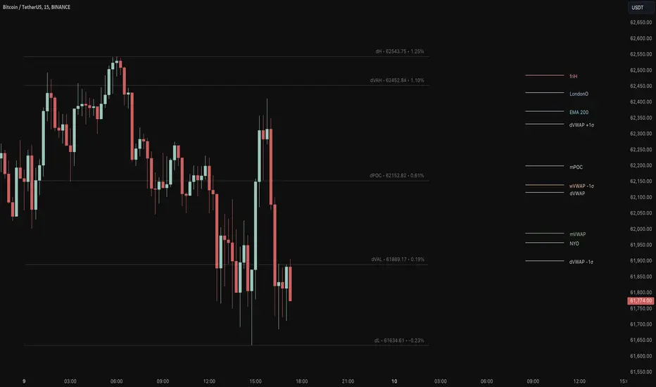
CRT overlay 2Overview
The "CRT overlay 2" is designed to plot key levels and detect market patterns based on the 4-hour candle around a specific start time (5AM). It incorporates elements like the high, low, and 50% level of a key 4-hour candle, and also tracks Fair Value Gaps (FVGs) to help identify potential price imbalances in the market. The indicator is primarily based on Candle Range Theory (CRT), which focuses on the significance of price movements within key candles and their relation to future market activity.
How the Script is Made
Key Components:
4-hour CRT Candle: The script identifies a specific 4-hour candle using a customizable start time (by default, it’s set to the 5 AM candle).
High, Low, and Midline Levels: For this selected 4-hour candle, the script calculates and draws the high, low, and 50% midpoint. These levels are used as reference points for further analysis.
Fair Value Gaps (FVGs): The script detects price gaps between candles (where the third candle does not fully overlap the first), which can act as areas of potential support or resistance. The user can toggle the plotting of midlines for these gaps.
Time Restrictions: The script limits its key functionalities (e.g., detecting highs, lows, and gaps) to a specific time window, between the target hour and the end hour (e.g., 5 AM to 10 AM).
Extensions and Visibility:
The plotted high, low, and midlines of the 4-hour candle extend a certain number of bars forward for visibility.
These lines stop extending after the end of the defined session (e.g., after 10 AM).
Wick Length Calculation:
The script calculates the length of a candle's wick as a percentage of the total range of the candle, which may provide insights into market rejections or momentum shifts.
Fair Value Gap (FVG) Detection:
The script detects both bullish and bearish FVGs based on a 3-candle pattern, plotting the gaps with customizable colors. The FVGs are then drawn on the chart for visual guidance.
Midlines of these gaps can also be drawn, and outdated or filled FVGs are removed after a set number of bars or if they are filled by price action.
How to Use It
Indicator Setup:
After adding the indicator to your chart, you will be able to customize settings for your desired timezone and the target 4-hour candle. By default, the script is set to the 5 AM candle, but this can be changed to any hour depending on your analysis needs.
The "CRT Candle Start" and "CRT Candle End" allow you to define the time range when the high, low, and midlines will be plotted and tracked.
Key Levels:
The script draws white lines for the high and low of the selected 4-hour candle, along with a green dashed line for the 50% mid-level. These lines serve as significant support and resistance levels.
During the defined session (e.g., 5 AM to 10 AM), these lines will actively extend and be visible on your chart.
After the session ends, these lines stop extending but remain on the chart for reference.
Fair Value Gaps (FVGs):
The script automatically identifies gaps between candles and plots them on the chart with colored boxes (green for bullish gaps, orange for bearish gaps). These areas can serve as potential reversal or continuation zones.
You can choose whether or not to plot a dashed line at the 50% mark of these FVGs. This midline can be important for targeting partial fills or retracements.
Sweep Alerts and Higher Highs/Lower Lows:
The script monitors price action to detect when the market forms the very first higher high or lower low within the high and low range of the 4-hour candle. When a higher high or lower low is detected, the script plots a yellow label on the chart to mark the event and triggers an alert.
These events can indicate potential sweep patterns or liquidity grabs.
FVG Removal:
The script includes a feature to automatically remove FVGs when they are filled by price action or after they become too old (based on a user-defined number of bars). This helps keep the chart clean for further analysis without clutter from outdated information.
Practical Application
Intraday Traders: The script helps traders focus on specific time windows (like 5 AM to 10 AM) and provides key reference levels (high, low, midline) that can guide trading decisions. Breaks and retests of these levels are common trading strategies.
Market Reversal and Continuation: The detection of Fair Value Gaps and higher highs/lower lows within the defined range can be useful for identifying potential reversal points or continuation signals in the market.
Candle Range Theory (CRT): The script is rooted in CRT, which emphasizes the importance of high and low levels of key candles for future price action. This theory is often used by traders looking to identify support/resistance zones or liquidity grabs in the market.
In summary, CRT overlay 2 is designed for precision trading around key timeframes, focusing on levels from the 4-hour candle and incorporating Fair Value Gaps for potential trade entries or exits. Its customizable inputs make it flexible for various strategies, and its focus on time-based levels is aligned with concepts in intraday trading and market structure analysis.

Price Action Smart Money Concepts [BigBeluga]THE SMART MONEY CONCEPTS Toolkit
The Smart Money Concepts [ BigBeluga ] is a comprehensive toolkit built around the principles of "smart money" behavior, which refers to the actions and strategies of institutional investors.
The Smart Money Concepts Toolkit brings together a suite of advanced indicators that are all interconnected and built around a unified concept: understanding and trading like institutional investors, or "smart money." These indicators are not just randomly chosen tools; they are features of a single overarching framework, which is why having them all in one place creates such a powerful system.
This all-in-one toolkit provides the user with a unique experience by automating most of the basic and advanced concepts on the chart, saving them time and improving their trading ideas.
Real-time market structure analysis simplifies complex trends by pinpointing key support, resistance, and breakout levels.
Advanced order block analysis leverages detailed volume data to pinpoint high-demand zones, revealing internal market sentiment and predicting potential reversals. This analysis utilizes bid/ask zones to provide supply/demand insights, empowering informed trading decisions.
Imbalance Concepts (FVG and Breakers) allows traders to identify potential market weaknesses and areas where price might be attracted to fill the gap, creating opportunities for entry and exit.
Swing failure patterns help traders identify potential entry points and rejection zones based on price swings.
Liquidity Concepts, our advanced liquidity algorithm, pinpoints high-impact events, allowing you to predict market shifts, strong price reactions, and potential stop-loss hunting zones. This gives traders an edge to make informed trading decisions based on liquidity dynamics.
🔵 FEATURES
The indicator has quite a lot of features that are provided below:
Swing market structure
Internal market structure
Mapping structure
Adjustable market structure
Strong/Weak H&L
Sweep
Volumetric Order block / Breakers
Fair Value Gaps / Breakers (multi-timeframe)
Swing Failure Patterns (multi-timeframe)
Deviation area
Equal H&L
Liquidity Prints
Buyside & Sellside
Sweep Area
Highs and Lows (multi-timeframe)
🔵 BASIC DEMONSTRATION OF ALL FEATURES
1. MARKET STRUCTURE
The preceding image illustrates the market structure functionality within the Smart Money Concepts indicator.
➤ Solid lines: These represent the core indicator's internal structure, forming the foundation for most other components. They visually depict the overall market direction and identify major reversal points marked by significant price movements (denoted as 'x').
➤ Internal Structure: These represent an alternative internal structure with the potential to drive more rapid market shifts. This is particularly relevant when a significant gap exists in the established swing structure, specifically between the Break of Structure (BOS) and the most recent Change of High/Low (CHoCH). Identifying these formations can offer opportunities for quicker entries and potential short-term reversals.
➤ Sweeps (x): These signify potential turning points in the market where liquidity is removed from the structure. This suggests a possible trend reversal and presents crucial entry opportunities. Sweeps are identified within both swing and internal structures, providing valuable insights for informed trading decisions.
➤ Mapping structure: A tool that automatically identifies and connects significant price highs and lows, creating a zig-zag pattern. It visualizes market structure, highlights trends, support/resistance levels, and potential breakouts. Helps traders quickly grasp price action patterns and make informed decisions.
➤ Color-coded candles based on market structure: These colors visually represent the underlying market structure, making it easier for traders to quickly identify trends.
➤ Extreme H&L: It visualizes market structure with extreme high and lows, which gives perspective for macro Market Structure.
2. VOLUMETRIC ORDER BLOCKS
Order blocks are specific areas on a financial chart where significant buying or selling activity has occurred. These are not just simple zones; they contain valuable information about market dynamics. Within each of these order blocks, volume bars represent the actual buying and selling activity that took place. These volume bars offer deeper insights into the strength of the order block by showing how much buying or selling power is concentrated in that specific zone.
Additionally, these order blocks can be transformed into Breaker Blocks. When an order block fails—meaning the price breaks through this zone without reversing—it becomes a breaker block. Breaker blocks are particularly useful for trading breakouts, as they signal that the market has shifted beyond a previously established zone, offering opportunities for traders to enter in the direction of the breakout.
Here's a breakdown:
➤ Bear Order Blocks (Red): These are zones where a lot of selling happened. Traders see these areas as places where sellers were strong, pushing the price down. When the price returns to these zones, it might face resistance and drop again.
➤ Bull Order Blocks (Green): These are zones where a lot of buying happened. Traders see these areas as places where buyers were strong, pushing the price up. When the price returns to these zones, it might find support and rise again.
These Order Blocks help traders identify potential areas for entering or exiting trades based on past market activity. The volume bars inside blocks show the amount of trading activity that occurred in these blocks, giving an idea of the strength of buying or selling pressure.
➤ Breaker Block: When an order block fails, meaning the price breaks through this zone without reversing, it becomes a breaker block. This indicates a significant shift in market liquidity and structure.
➤ A bearish breaker block occurs after a bullish order block fails. This typically happens when there's an upward trend, and a certain level that was expected to support the market's rise instead gives way, leading to a sharp decline. This decline indicates that sellers have overcome the buyers, absorbing liquidity and shifting the sentiment from bullish to bearish.
Conversely, a bullish breaker block is formed from the failure of a bearish order block. In a downtrend, when a level that was expected to act as resistance is breached, and the price shoots up, it signifies that buyers have taken control, overpowering the sellers.
3. FAIR VALUE GAPS:
A fair value gap (FVG), also referred to as an imbalance, is an essential concept in Smart Money trading. It highlights the supply and demand dynamics. This gap arises when there's a notable difference between the volume of buy and sell orders. FVGs can be found across various asset classes, including forex, commodities, stocks, and cryptocurrencies.
FVGs in this toolkit have the ability to detect raids of FVG which helps to identify potential price reversals.
Mitigation option helps to change from what source FVGs will be identified: Close, Wicks or AVG.
4. SWING FAILURE PATTERN (SFP):
The Swing Failure Pattern is a liquidity engineering pattern, generally used to fill large orders. This means, the SFP generally occurs when larger players push the price into liquidity pockets with the sole objective of filling their own positions.
SFP is a technical analysis tool designed to identify potential market reversals. It works by detecting instances where the price briefly breaks a previous high or low but fails to maintain that breakout, quickly reversing direction.
How it works:
Pattern Detection: The indicator scans for price movements that breach recent highs or lows.
Reversal Confirmation: If the price quickly reverses after breaching these levels, it's identified as an SFP.
➤ SFP Display:
Bullish SFP: Marked with a green symbol when price drops below a recent low before reversing upwards.
Bearish SFP: Marked with a red symbol when price rises above a recent high before reversing downwards.
➤ Deviation Levels: After detecting an SFP, the indicator projects white lines showing potential price deviation:
For bullish SFPs, the deviation line appears above the current price.
For bearish SFPs, the deviation line appears below the current price.
These deviation levels can serve as a potential trading opportunity or areas where the reversal might lose momentum.
With Volume Threshold and Filtering of SFP traders can adjust their trading style:
Volume Threshold: This setting allows traders to filter SFPs based on the volume of the reversal candle. By setting a higher volume threshold, traders can focus on potentially more significant reversals that are backed by higher trading activity.
SFP Filtering: This feature enables traders to filter SFP detection. It includes parameters such as:
5. LIQUIDITY CONCEPTS:
➤ Equal Lows (EQL) and Equal Highs (EQH) are important concepts in liquidity-based trading.
EQL: A series of two or more swing lows that occur at approximately the same price level.
EQH: A series of two or more swing highs that occur at approximately the same price level.
EQLs and EQHs are seen as potential liquidity pools where a large number of stop loss orders or limit orders may be clustered. They can be used as potential reverse points for trades.
This multi-period feature allows traders to select less and more significant EQL and EQH:
➤ Liquidity wicks:
Liquidity wicks are a minor representation of a stop-loss hunt during the retracement of a pivot point:
➤ Buy and Sell side liquidity:
The buy side liquidity represents a concentration of potential buy orders below the current price level. When price moves into this area, it can lead to increased buying pressure due to the execution of these orders.
The sell side liquidity indicates a pool of potential sell orders below the current price level. Price movement into this area can result in increased selling pressure as these orders are executed.
➤ Sweep Liquidation Zones:
Sweep Liquidation Zones are crucial for understanding market structure and potential future price movements. They provide insights into areas where significant market participants have been forced out of their positions, potentially setting up new trading opportunities.
🔵 USAGE & EXAMPLES
The core principle behind the success of this toolkit lies in identifying "confluence." This refers to the convergence of multiple trading indicators all signaling the same information at a specific point or area. By seeking such alignment, traders can significantly enhance the likelihood of successful trades.
MS + OBs
The chart illustrates a highly bullish setup where the price is rejecting from a bullish order block (POC), while simultaneously forming a bullish Swing Failure Pattern (SFP). This occurs after an internal structure change, marked by a bullish Change of Character (CHoCH). The price broke through a bearish order block, transforming it into a breaker block, further confirming the bullish momentum.
The combination of these elements—bullish order blocks, SFP, and CHoCH—creates a powerful bullish signal, reinforcing the potential for upward movement in the market.
SFP + Bear OB
This chart above displays a bearish setup with a high probability of a price move lower. The price is currently rejecting from a bear order block, which represents a key resistance area where significant selling pressure has previously occurred. A Swing Failure Pattern (SFP) has also formed near this bear order block, indicating that the price briefly attempted to break above a recent high but failed to sustain that upward movement. This failure suggests that buyers are losing momentum, and the market could be preparing for a move to the downside.
Additionally, we can toggle on the Deviation Area in the SFP section to highlight potential levels where price deviation might occur. These deviation areas represent zones where the price is likely to react after the Swing Failure Pattern:
BUY – SELL sides + EQL
The chart showcases a bullish setup with a high probability of price breaking out of the current sell-side resistance level. The market structure indicates a formation of Equal Lows (EQL), which often suggests a build-up of liquidity that could drive the price higher.
The presence of strong buy-side pressure (69%), indicated by the green zone at the bottom, reinforces this bullish outlook. This area represents a key support zone where buyers are outpacing sellers, providing the foundation for a potential upward breakout.
EQL + Bull ChoCh
This chart illustrates a potential bullish setup, driven by the formation of Equal Lows (EQL) followed by a bullish Change of Character (CHoCH). The presence of Equal Lows often signals a liquidity build-up, which can lead to a reversal when combined with additional bullish signals.
Liquidity grab + Bull ChoCh + FVGs
This chart demonstrates a strong bullish scenario, where several important market dynamics are at play. The price begins its upward momentum from Liquidity grab following a bullish Change of Character (CHoCH), signaling the transition from a bearish phase to a bullish one.
As the price progresses, it performs liquidity grabs, which serve to gather the necessary fuel for further movement. These liquidity grabs often occur before significant price surges, as large market participants exploit these areas to accumulate positions before pushing the price higher.
The chart also highlights a market imbalance area, showing strong momentum as the price moves swiftly through this zone.
In this examples, we see how the combination of multiple “smart money” tools helps identify a potential trade opportunities. This is just one of the many scenarios that traders can spot using this toolkit. Other combinations—such as order blocks, liquidity grabs, fair value gaps, and Swing Failure Patterns (SFPs)—can also be layered on top of these concepts to further refine your trading strategy.
🔵 SETTINGS
Window: limit calculation period
Swing: limit drawing function
Mapping structure: show structural points
Algorithmic Logic: (Extreme-Adjusted) Use max high/low or pivot point calculation
Algorithmic loopback: pivot point look back
Show Last: Amount of Order block to display
Hide Overlap: hide overlapping order blocks
Construction: Size of the order blocks
Fair value gaps: Choose between normal FVG or Breaker FVG
Mitigation: (close - wick - avg) point to mitigate the order block/imbalance
SFP lookback: find a higher / lower point to improve accuracy
Threshold: remove less relevant SFP
Equal H&L: (short-mid-long term) display longer term
Liquidity Prints: Shows wicks of candles where liquidity was grabbed
Sweep Area: Identify Sweep Liquidation areas
By combining these indicators in one toolkit, traders are equipped with a comprehensive suite of tools that address every angle of the Smart Money Concept. Instead of relying on disparate tools spread across various platforms, having them integrated into a single, cohesive system allows traders to easily see confluence and make more informed trading decisions.

Previous Highs & Lows [LuxAlgo]The Previous Highs & Lows indicator highlights a user-set amount of previous maximum/minimum prices made within specific intervals, these are displayed as levels customizable levels.
Additionally, one upper and lower zone constructed from the previously displayed highs/lows is included, providing support/resistance areas.
🔶 USAGE
Previous highs/lows are often perceived as key trading levels with the potential of generating multiple reactions upon being reached.
While the daily interval is more commonly used, users can use different intervals, with the indicator supporting hourly, daily, weekly, monthly, and yearly intervals. Using higher intervals on low timeframes can return more distant levels relative to the most recent price, which might not be relevant.
Each level is numbered, with more recent previous highs/lows having a lower number associated with them, users can also highlight more recent levels through a transparency gradient.
Users can control the amount of previous highs/lows displayed using the "Show Last" settings, with a higher value providing more potential support/resistance. Returned previous highs/lows can eventually be filtered out based on their position by enabling the "Filter Based On Position" setting, only keeping previous highs above the current closing price and previous lows below the current closing price, giving more relevant levels as a result.
🔹 Previous High/Low Areas
The indicator includes two areas constructed from the respective percentiles of the returned previous highs/lows. These can be useful as more general support/resistance areas.
Wider areas are often indicative of a group of previous highs or lows being more dispersed, resulting in areas that are easier to reach. Wider areas can also be obtained by increasing the "Areas Width" setting.
Note: Areas will only be displayed if "Show Last" is greater than 1
🔶 SETTINGS
Show Last: Determines the amount of more recent previous highs and previous low levels displayed by the indicator.
Interval: Interval used to capture maximum/minimum price values,
Areas Width: Width of the displayed top/bottom areas, with higher values returning wider areas.
Filter Based On Position: When enabled only display previous highs above the current closing price and previous lows below the current closing price.
🔹 Style
Minimum Gradient Transparency: Minimum transparency value applied to the colors of the oldest displayed previous highs/lows levels.
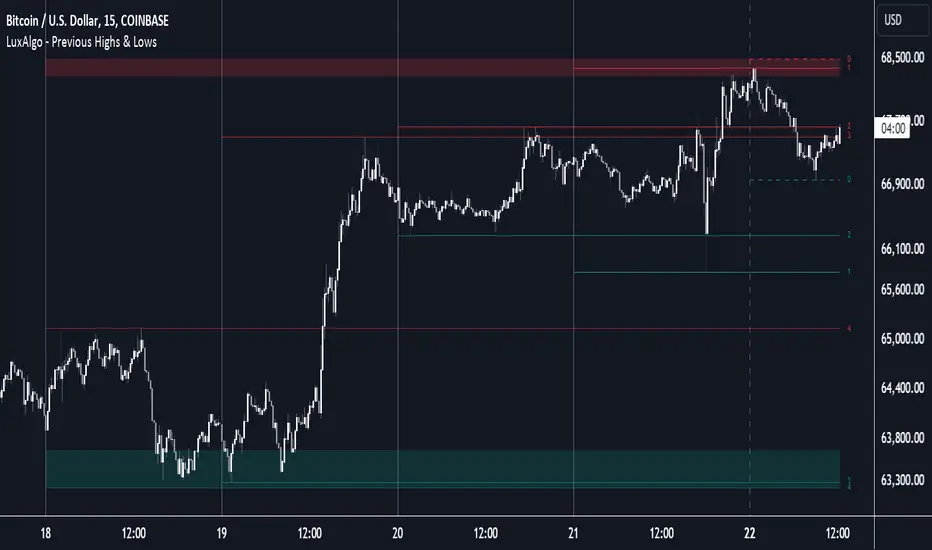
RunRox - Advanced SMC⭐️ Introducing Our Advanced SMC Indicator: Elevate Your Smart Money Concept Trading
We are excited to present our innovative indicator, specifically designed for the Smart Money Concept (SMC). Our approach goes beyond the traditional SMC strategy by offering significant enhancements that can help you achieve stronger trading performance.
We employ a more sophisticated SMC structure, incorporating improved IDM (Inducement) logic, both internal and external structures, and four types of order blocks. This allows for deeper insights into market trends and a clearer understanding of how major market participants may be manipulating price action.
🟠 Indicator Features:
Structure
HTF Structure – Choose any timeframe and display its structure on your current chart.
CHoCH | BOS | IDM – Display any components from this structure.
Market Minor Structure – Swing and Minor structure.
BOS/CHoCH Breaking by (Body | Wick) – Choose the principle for building the structure, either by the candle body or by their wicks.
BOS/CHoCH Move if Swept – When liquidity is taken, decide whether to move the structure line higher or consider it a structural break.
Move CHoCH/BOS – Relocate key points on the chart if the structure becomes too large.
FVG Concept
HTF FVG – Choose any timeframe from which you want to display FVG on your current chart
Three Types of FVG – Classic FVG, Double FVG, Implied Imbalance
Reaction to FVG – Show the market’s reaction to FVG on the chart
Mitigation Method – Select the fill method that suits your approach (Touch/Midline/Complete)
Remove Filled FVG – Remove FVGs from the chart once they have been filled
Combine FVG – Merge several consecutive FVGs into one
Length FVG – Adjust the number of candles that define the FVG
OrderBlock Concept
HTF OrderBlock – Choose any timeframe from which you want to display orderblocks on your current chart
Swing and Minor Orderblocks – Display only the orderblocks you need, whether from the Swing or Minor structure
Four Types of Order Blocks – Advanced OB, Classic OB, BTS/STB zones, Extremum Candle
Block Based on – Decide whether to base the orderblock on candle highs/lows or candle open/close
Mitigation Method – Define when an orderblock is considered filled (Touch/Midline/Complete)
Remove Blocks Older – Remove older orderblocks from the chart
Hide Overlap – Disable overlapping orderblocks when they appear in the same area
Eat Young Blocks – Reduce the size of an orderblock until it fully forms
Hide Distant Blocks – Remove orderblocks that are too far from the current price
Previous Highs & Lows
Four Level Types – Day, Week, Month, Quarter
Style Customization – Choose line color, line style, and transparency
Fibonacci Retracements
10 Template Options – Ten different bases on which you can build your Fibonacci grid
Up to 7 Levels – Add up to seven Fibonacci levels for your convenience
Fibo Inversion – Option to invert the Fibonacci grid
Style Customization – Choose line colors, line styles, and transparency
Additional Functions
Premium & Discount Zones – A popular concept we’ve incorporated to help identify potential trading areas within premium or discount prices
Equal Highs & Lows – High-liquidity levels where market makers may seek liquidity
Color Candles – Automatically colors candles based on the current trend
Market Structure ZigZag – Offers a clear visual of the zigzag pattern on which the structure is built
Key Point Labels – Displays important swing high/low points directly on the chart
General Styling – Customize any chart element, including size, style, color, and transparency
Alert Customization – Over 16 types of alerts, easily configured in a few clicks. Receive only the notifications you need. Custom alerts are also available for developers.
Next, we will provide a detailed overview of all the indicator’s features, accompanied by chart examples.
📈 Structure
What Is IDM?
IDM, or the Institutional Distribution Model, is an advanced concept within SMC that focuses on how institutional players distribute their positions in the market. By analyzing IDM, traders can better anticipate price movements and potential turning points, thereby gaining a meaningful edge in their trading.
In our structure concept, IDM can form under specific conditions. The market does not always provide a high-liquidity point to work with, so we’ve adopted a flexible approach. We generate IDM when a certain type of liquidity appears during the impulse and BOS break, allowing for a potential future liquidity sweep.
Below, I will provide an example that illustrates when IDM forms as a liquidity magnet within the structure - and when it does not.
As shown in the example above, we focus on the initial impulse after the BOS. If liquidity forms during this impulse - liquidity that needs to be taken out during the structural move - we mark an IDM level as a price magnet. However, if this liquidity does not appear, we do not create an IDM. In that case, the same point might serve as an FVG or play a different role, depending on your trading approach.
This concept makes the structure more flexible and better able to respond immediately to market movements and key structural points.
Above is an example on the chart illustrating what the structure looks like both with and without IDM. As you can see, when the structural move includes pullbacks and consolidation, there is an opportunity to form an IDM as a price magnet. However, if the impulses are strong and lack pullbacks, FVG becomes the only magnet in that move. Depending on the chart, our indicator adapts to the current market conditions and highlights potential liquidity collection points.
📊 Swing and Minor Structure
In the new version of the indicator, the minor structure and the swing structure differ from each other.
Swing structure - In this structure, as mentioned earlier, the IDM concept remains a price magnet and is formed at certain points on the chart if the conditions allow. If these points do not appear, IDM might not form at all.
Minor structure - Here, we have completely removed IDM and only kept BOS and CHoCH for structure formation. We found that for a minor structure, this approach allows faster reactions to trend changes, depending on market movements.
By making these adjustments, we have resolved the main issue of the advanced structure, which was the large distance between BOS and CHoCH that sometimes resulted in a month-long consolidation between these levels. In this version, those problems no longer occur.
If, for some reason, your settings result in a larger swing structure, you can still work with the minor structure using the same POI as in the swing structure. OrderBlock and FVG remain the primary drivers of order flow.
Shown above is a screenshot of the main structure settings you can adjust. These settings are highly flexible and can be tailored to fit a wide range of trading preferences.
⚖️ FVG Concept
A new feature of our indicator is the FVG concept. We automatically detect three types of FVG at the moment, which will be explained below.
FVG - the standard Fair Value Gap
Double FVG - a double FVG, also referred to as BPR (Balanced Price Range)
Implied Imbalance - a type of imbalance that arises from buyer or seller demand
Below, we will look at examples of the FVG types we currently identify.
All price inefficiencies work in real time, immediately appearing on the chart and allowing traders to quickly respond to FVG reactions.
We have also enhanced this concept by displaying FVG reactions on the chart. If an FVG triggers a reaction and the price responds to that range, we highlight it on the chart, so you can recognize the reaction and make timely trading decisions. A screenshot below shows how this looks in practice.
Below is a screenshot illustrating the main settings of this concept, along with detailed descriptions.
📦 OrderBlock Concept
OrderBlocks provide an effective way to identify areas of interest and make informed decisions. We have dedicated significant effort to refining this section’s functionality and have achieved strong results in doing so.
Order Block Types
Advanced OrderBlock – A specialized type of order block generated by our internal algorithm. This can help traders aim for tighter entries and potentially more favorable risk-reward ratios within a narrow price range.
OrderBlock – The classic type, formed at the highs or lows of a structure when a BOS or CHoCH occurs. It can still be an effective entry method but typically spans a wider price range.
Extremum Candle – Based on liquidity grabs. The candle creating this order block must collect liquidity before making an impulsive move that breaks the BOS or CHoCH.
BTS / STB (Buy To Sell / Sell To Buy) – This concept may appear when market makers manipulate price to buy or sell an asset. It often covers a larger price range because it relies on a brief impulsive move to form.
Each type of order block has its own strengths and weaknesses. We provide traders with the flexibility to choose which types suit their trading style and preferences.
Above is an example of how you can apply OrderFlow alongside our structure and orderblocks, which can produce solid results when combined with the Smart Money concept.
In this demonstration, we have highlighted the Advanced Orderblock as an illustration.
Above is a screenshot of all the settings related to this section. They can be customized to suit your specific needs, ensuring you only see what is genuinely relevant on your chart.
📏 Previous Highs and Lows
You can select four levels to display on the chart as some of the most liquid zones:
Daily Highs and Lows
Weekly Highs and Lows
Monthly Highs and Lows
Quarterly Highs and Lows
This feature helps you identify important levels on lower timeframes and focus on these zones for potential trading opportunities. Below is an example of how it appears on the chart.
Below, you can see the settings available in this section.
📐 Fibonacci Levels
Likewise, a new section in our indicator is Fibonacci Levels, a well-known tool recognized as a reliable source of important levels on the chart. We have added this functionality with the option to choose how you want to generate these levels and which specific levels you want to display.
You can plot Fibonacci levels based on the Swing structure, Minor structure, previous or current day, month, and more. In total, there are 10 different options for constructing the Fibonacci grid.
Above, you can see an example of how it appears on the chart, and below you will find the settings available in this section.
🈹 Premium and Discount
Another useful feature for all traders is the Premium and Discount zones based on structure. This makes it easy to identify areas of interest—whether in a discount or premium zone, or in an equilibrium area.
Below, you can also see the settings available in this section.
✅ Additional Function
We have also separated a few functions into their own section:
Color Candles – Colors the candles according to the current trend.
Market Structure ZigZag – Visually highlights the zigzag used to form the structure.
Key Point Labels – Displays the points on the chart from which the structure is built.
Equal Highs & Lows – Identifies equal highs and lows as areas of potential liquidity for larger market players, as price often aims to sweep these zones.
Below are a few screenshots showing how these features appear on the chart.
Color Candles
Market Structure ZigZag and Key Point Labels
Equal Highs & Lows
Below, you can see a screenshot displaying all the settings available in this section.
🎨 General Styling
We have devoted considerable effort to providing flexible customization for each element on the chart, so you can design the exact look you want. That’s why we created an additional section where you can adjust any element’s size, style, and more.
Combined with extensive color and transparency options, this feature provides a flexible appearance for the indicator on any chart.
Below, you can see the settings available in this section
🔔 Alert Customization
You can configure over 16 types of reactions to various events on the chart. Additionally, you can set up alerts to trigger at specific fill levels and explore numerous other alert options, as shown in the screenshot below.
🟠 Usage Examples
We have also prepared several examples of how to use the indicator. These are standard entry models taken from the classic Smart Money concept.
First Example
In the screenshot above, the market displays a downward structure until a manipulation occurs, followed by a CHoCH break. This is a standard entry model featuring an entry at the nearest FVG, a stop-loss placed beyond the manipulation, and a target at the nearest liquidity zone—whether session-based or, as in our case, a gap (one of the FVG types) that price commonly revisits.
This is considered a more aggressive entry because we only waited for a single confirmation of the trend change—the CHoCH break—and then entered immediately afterward. While the WinRate might be lower in such trades, the Risk-Reward ratio is typically very high if you correctly identify the manipulation.
Second Example
This approach is more conservative and less risky, typically offering a higher WinRate but with a lower Risk-Reward ratio.
Here, we use the 4H FVG as our decision point (POI). With the indicator, we plot the 4-hour FVG on our current chart without needing to switch back and forth between timeframes.
Once price reaches our POI, we look for an entry model that includes three confirmations:
First Confirmation – A CHoCH break.
Second Confirmation – A manipulation.
Third Confirmation – A second BOS break.
We wait for all these confirmations before entering the trade, ensuring our stop-loss is well-protected since the remaining liquidity has been swept and the 4-hour FVG has been fully filled.
Our target is the full fill of a higher timeframe FVG or other high-liquidity levels below.
In a conservative setup, it is crucial to allow a complete OrderFlow to develop, including manipulations and clear breaks of lower levels. This approach helps protect the trade and often results in a higher WinRate.
🟠 Disclaimer
Past performance is not indicative of future results. To trade successfully, it is crucial to have a thorough understanding of the market context and the specific situation at hand. Always conduct your own research and analysis before making any trading decisions.
To gain access to the indicator, please review the author's instructions below this post

[TA] Breaker BlocksDescription:
The Breaker Blocks Finder is a sophisticated tool designed for traders who seek to identify key market structures algorithmically. This indicator meticulously scans for both bullish and bearish breaker blocks, visually delineating them on the chart for easy identification.
Exploring ICT Breaker Blocks: Enhancing Your Trading with Precision
Understanding ICT Breaker Blocks: ICT Breaker Blocks are a nuanced trading concept that leverages market liquidity and manipulation to identify potential breakout points. This strategy is particularly effective in pinpointing moments where the market is poised for a significant directional move.
Mechanics of ICT Breaker Blocks: The essence of this strategy lies in detecting manipulation phases where liquidity is being accumulated, typically around critical market highs or lows. This setup leads to a Stop Hunt, a tactical move to trigger stop orders and fuel a breakout in the opposite direction.
Detailed Breakdown of Breaker Block Types:
Bullish Breaker Blocks:
• Bullish Order Block: The precursor to a bullish breakout, setting the stage for a potential upward move.
• Bullish Breaker Candle: An upward-closing candle that forms just before breaking past an old low, signaling a bullish reversal.
• Confirmation: Achieved when the price dips below the prior low and subsequently rises above the high of the swing, solidifying the bullish breakout.
• Identification: Look for a failed bearish order block, indicated by an initial drop in prices that ultimately reverses, hinting at a bullish shift.
• Key Elements: Monitor the pattern of lows and highs (low, high, lower low, higher high), which suggests an emerging bullish trend.
Bearish Breaker Blocks:
• Bearish Breaker Candle: A downward-closing candle that appears right before an old high is surpassed, indicating a bearish reversal.
• Confirmation: Occurs when prices climb above the previous high and then descend below the swing's low, confirming the bearish move.
• Identification: Initiate by identifying a failed bullish order block, where initial upward price momentum falters and reverses, signaling bearish potential.
• Key Elements: Focus on the sequence of highs and lows (high, low, higher high, lower low), which may denote a looming bearish trend.
Spotting High Probability Breaker Blocks: To enhance the reliability of breaker block identification, incorporate patterns that exhibit a Fair Value Gap (FVG), which typically indicates a stronger likelihood of a successful breakout.
Leveraging ICT Breaker Blocks in Trading: Our Inner Circle Trading mentorship delves into these concepts and more, providing you with comprehensive education and weekly market insights.
By mastering ICT Breaker Blocks, you're equipped with a powerful tool to navigate the intricacies of the market, making informed and strategic trading decisions.
This channel provides you with comprehensive education and weekly market insights. If you enjoyed this thread, like, share, and follow. Join us for an in-depth exploration of advanced trading strategies, and elevate your trading proficiency.
Still confused about Breaker Blocks?
Follow these steps for Bullish Breaker Blocks and reverse them for Bearish Breaker Blocks.
Think:
Bullish BB = Low, High, Lower Low, then Higher High
Bearish BB = High, Low, Higher High, then Lower Low
While this tool is a powerful addition to your trading strategy, it's important to note that it is not an autotrader. Traders should use this indicator as part of a comprehensive trading plan, considering other market factors and personal risk tolerance.
Risk Disclaimer:
Trading financial markets involves significant risk and can result in the loss of your invested capital. You should not invest more than you can afford to lose and should ensure that you fully understand the risks involved. Before trading, please take into consideration your level of experience, investment objectives, and seek independent financial advice if necessary. This indicator is provided as-is without any guarantees or warranty. Use of this indicator is at your own risk, and the creator is not responsible for any financial losses or damages.
