[Pandora] Laguerre Ultimate Explorations MulticatorIt's time to begin demonstrations differentiating the difference between known and actual feasibility beyond imagination... Welcome to my algorithmic twilight zone .
INTRODUCTION:
Hot off my press, I present this Laguerre multicator employing PSv6.0, originally formulated by John Ehlers for TASC - July 2025 Traders Tips. Basically I transcended Ehlers' notions of transversal filtration with an overhaul of his Laguerre design with my "what if" Pandora notions included. Striving beyond John Ehlers' original intended design. This action packed indicator is a radically revamped version of his original filter using novel techniques. My aim was to explore whether providing even more enhanced responsiveness and lesser lag is possible and how. Presented here is my mind warping results to witness.
EHLERS' LAGUERRE EXPLAINED:
First and foremost, the concept of Ehlers' Laguerre-izing method deserves a comprehensive deep dive. Ehlers' Laguerre filter design, as it functions originally, begins with his Ultimate Smoother (US) followed by a gang of four LERP (jargon for Linear intERPolation) filters. Following a myriad of cascading LERPs is a window-like FIR filter tapped into the LERP delay values to provide extra smoothness via the output.
On a side note, damping factor controlled LERP filters resemble EMAs indeed, but aren't exactly "periodic" filters that would have a period/length parameter and their subsequent calculations. I won't go into fine-grained relationship details, but EMA and LERP are indeed related in approach, being cousins of similar pedigree.
EXAMINING LAGUERRE:
I focused firstly on US initialization obstacles at Pine's bar_index==0 with nz() in abundance. The next primary notion of intrigue I mostly wondered about was, why are there four LERP elements instead of fewer or more. Why not three or why not two LERPs, etc... 1-4-6-4-1, I remember seeing those coefficients before in high pass filters.
Gathering my thoughts from that highpass knowledge base, I devised other tapped configuration modes to inspect their behavior out of curiosity. Eureka! There is actually more to Laguerre than Ehlers' mind provided, now that I had formulated additional modes. Each mode exhibits it's own lag/smoothness characteristics better than the quad LERPed version. I narrowed it down to a total of 5 modes for exploration. Mode 0 is just the raw US by itself.
ANALYZING FILTER BEHAVIORS:
Which option might be possibly superior, and how may I determine that? Fortunately, I have a custom-built analyzer allowing me to thoroughly examine transient responses across multiple periodicities simultaneously, providing remarkable visual insights.
While Ehlers has meagerly touched upon presenting general frequency responses in his books, I have excelled far beyond that. This robust filter analysis capability enables me to observe finer aspects hidden to others, ultimately leading to the deprecation of numerous existing filters. Not only this, but inventing entirely new species of filtration whether lowpass, highpass, or bandpass is already possible with a thorough comprehensive evaluation.
Revealing what's quirky with each filter and having the ability to discover what filters may be lacking in performance, is one of it's implications. I'm just going to explain this: For example US has a little too much overshoot to my liking, along with nonconformant cutoff frequency compliance with the period parameter. Perhaps Ehlers should inspect US coefficients a bit closer... I hope stating this is not received in an ill manner, as it's not my intention here.
What this technically eludes to is that UltimateSmoother can be further improved, analogous to my Laguerre alterations described above. I will also state Laguerre can indeed be reformulated to an even greater extent concerning group delay, from what I have already discussed. Another exciting time though... More investigative research is warranted.
LAGUERRE CONCLUSIONS:
After analyzing Laguerre's frequency compliance, transient responses, amplitudes, lag, symmetry across periodicities, noise rejection, and smoothness... I favor mode 3 for a multitude of reasons over the mode 4 configuration, but mostly superb smoothing with less lag, AND I also appreciated mode 1 & 2 for it's lower lag performance options.
Each mode and lag (phase shift) damping value has it's own unique characteristics at extremes, yet they demonstrate additional finesse in it's new hybrid form without adding too much more complexity. This multicator has a bunch of Laguerre filters in the overlay chart over many periodicities so you can easily witness it's differing periodic symmetries on an input signal while adjusting lag and mode.
LAGUERRE OSCILLATOR:
The oscillator is integrated into the laguerreMulti() function for the intention of posterity only. I performed no evaluation on it, only providing the code in Pine. That wasn't part of my intended exploration adventure, as I'm more TREND oriented for the time being, focusing my efforts there.
Market analysis has two primary aspects in my observations, one cyclic while the other is trending dynamics... There's endless oscillators, but my expectations for trend analysis seems a little lesser explored in my opinion, hence my laborious trend endeavors. Ehlers provided both indicator facets this time around, and I hope you find the filtration aspect more intriguing after absorption of this reading.
FUNCTION MODULES EXPLAINED:
The Ultimate Smoother is an advanced IIR lowpass smoothing filter intended to minimize noise in time series data with minimal group delay, similar to a traditional biquad filter. This calculation helps to create a smoother version of the original signal without the distortions of short-term fluctuations and with minimal lag, adjustable by period.
The Modified Laguerre Lowpass Filter (MLLF) enhances the functionality of US by introducing a Laguerre mode parameter along side the lag parameter to refine control over the amount of additional smoothing/lag applied to the signal. By tethering US with this LERPed lag mechanism, MLLF achieves an effective balance between responsiveness and smoothness, allowing for customizable lag adjustments via multiple inputs. This filter ends with selecting from a choice of weighted averages derived from a gang of up to four cascading LERP calculations, resulting with smoother representations of the data.
The Laguerre Oscillator is a momentum-like indicator derived from the output of US and a singular LERPed lowpass filter. It calculates the difference between the US data and Laguerre filter data, normalizing it by the root mean square (RMS). This quasi-normalization technique helps to assess the intensity of the momentum on any timeframe within an expected bound range centered around 0.0. When the Laguerre Oscillator is positive, it suggests that the smoothed data is trending upward, while a negative value indicates a downward trend. Adjustability is controlled with period, lag, Laguerre mode, and RMS period.
Pesquisar nos scripts por "ha溢价率"

Inflection PointInflection Point - The Adaptive Confluence Reversal Engine
This is not just another peak and valley indicator; it is a complete and total reimagining of how market turning points are detected, qualified, and acted upon. Born from the foundational concepts explored in systems like my earlier creation, DAFE - Turning Point, Inflection Point is a ground-up engineering feat designed for the modern trader. It moves beyond static rules and simple pattern recognition into the realm of dynamic, multi-factor confluence analysis and adaptive machine learning.
Where other indicators provide a guess, Inflection Point provides a probability. It meticulously analyzes the market's deepest currents—momentum, exhaustion, and reversal velocity—and fuses them into a single, unified "Confluence Score." This is not a simple combination of indicators; it is an intelligent, weighted system where each component works in concert, creating an analytical engine that is orders of magnitude more sophisticated and reliable than any standard reversal tool.
Furthermore, Inflection Point learns. Through its advanced Adaptive Learning Engine, it constantly monitors its own performance, adjusting its confidence and selectivity in real-time based on its recent success rate. This allows it to adapt its behavior to any security, on any timeframe, with remarkable success.
Theoretical Foundation - Confluence Core
Inflection Point's predictive power does not come from a single, magical formula. It comes from the intelligent synthesis of three critical market phenomena, weighted and scored in real-time to generate a single, high-conviction probability rating.
1. Factor One: Pre-Reversal Momentum State (RSI Analysis)
Instead of reacting to a simple RSI cross, Inflection Point proactively scans for the build-up of momentum that precedes a reversal.
• Formulaic Concept: It measures the highest RSI value over a lookback period for peaks and the lowest RSI for valleys. A signal is only considered valid if significant momentum has been established before the turn, indicating a stretched market condition ripe for reversal.
• Asymmetric Sophistication: The engine uses different, optimized thresholds for bull and bear momentum, recognizing that markets often fall faster than they rise.
2. Factor Two: Volatility Exhaustion (Bollinger Band Analysis)
A true reversal often occurs when price makes a final, exhaustive push into unsustainable territory.
• Formulaic Concept: The engine detects when price has significantly pierced the outer Bollinger Bands. This is not just a touch, but a statistical deviation from the mean that signals volatility exhaustion, where the energy for the current move is likely depleted.
3. Factor Three: Reversal Strength (Rate of Change Analysis)
The character of a reversal matters. A sharp, decisive turn is more significant than a slow, meandering one.
• Formulaic Concept: Using a short-term Rate of Change (ROC), the engine measures the velocity of the reversal itself. A higher ROC score adds significant weight to the final probability, confirming that the new direction has conviction.
4. The Final Calculation: The Adaptive Learning Engine
This is the system's "brain." It maintains a history of its past signals and calculates its real-time win rate. This hitRate is then used to generate an adaptiveMultiplier.
• Self-Correction: In "Quality Control" mode, a high win rate makes the indicator more selective, demanding a higher probability score to issue a signal, thereby protecting streaks. A lower win rate makes it slightly less selective to ensure it continues learning from new market conditions.
• The result is a system that is not static, but a living, breathing tool that adapts its personality to the unique rhythm of any chart.
Why Inflection Point is a Paradigm Shift
Inflection Point is fundamentally different from other reversal indicators for three key reasons:
Confluence Over Isolation: Standard indicators look at one thing (e.g., RSI > 70). Inflection Point simultaneously analyzes momentum, volatility, and velocity, understanding that true reversals are a product of multiple converging factors. It answers not just "if," but "why" a reversal is likely.
Probabilistic Over Binary: Other tools give you a simple "yes" or "no." Inflection Point provides a probability score from 0-100, allowing you to gauge the conviction of every potential signal. This empowers you to differentiate between a weak setup and an A+ opportunity.
Adaptive Over Static: Every other indicator uses the same rules forever. Inflection Point's Adaptive Engine means it is constantly refining its own logic based on what is actually working in the current market, on the specific asset you are trading. It is tailored to the now.
The Inputs Menu - Your Command Center
Every setting is a lever of control, allowing you to tune the engine to your precise trading style and market focus.
🧠 Neural Core Engine
Analysis Depth: This is the primary lookback for the Bollinger Band and other core calculations. A shorter depth makes the indicator faster and more sensitive, ideal for scalping. A longer depth makes it slower and more stable, ideal for swing trading.
Minimum Probability %: This is your master signal filter. It sets the minimum Confluence Score required to plot a signal. Higher values (85-95) will give you only the highest-conviction A+ setups. Lower values (70-80) will show more potential opportunities.
🤖 Adaptive Neural Learning
Enable Adaptive Learning Engine: Toggles the entire learning system. Disabling it will make the indicator's logic static.
Peak/Valley Success Threshold (ATR): This defines what constitutes a "successful" trade for the learning engine. A value of 1.5 means price must move 1.5x the ATR in your favor for the signal to be marked as a win. Adjust this to match your personal take-profit strategy.
Adaptive Mode: This dictates how the engine uses its hitRate. "Quality Control" is recommended for its intelligent filtering. "Aggressive" will always boost signal scores, useful for finding more setups in a known, trending environment.
Asymmetric Balance: Allows you to apply a "boost" to either peak (short) or valley (long) signals. If you find the market you're trading has stronger long reversals, you can increase the "Valley Signal Boost" to catch them more effectively.
🛡️ Elite Filters
Market Noise Filter: An exceptional tool for avoiding choppy markets. It counts the number of directional changes in the last 5 bars. If the market is whipping back and forth too much, it will block the signal. Lower the "Max Direction Changes" to be extremely selective.
Volume Filter: Requires signal confirmation from a significant volume spike. The "Volume Multiplier" dictates how large this spike must be (e.g., 1.2 = 20% above average volume). This is invaluable for filtering out low-conviction moves in stocks and crypto.
The Dashboard - Your Analytical Co-Pilot
The dashboard is not just a set of numbers; it is a holistic overview of the market's health and the engine's current state.
Unified AI Score: This section provides the most critical, at-a-glance information. "Total Score" is the current probability reading, while "Quality" gives you a human-readable interpretation. "Win Rate" shows the real-time performance of the Adaptive Engine.
Order Flow (OFPI): This measures the "weight" of money behind recent price moves by analyzing price change relative to volume. A high positive OFPI suggests strong buying pressure, while a high negative value suggests strong selling pressure. It gives you a peek into the market's underlying flow.
Component Analysis: This allows you to see the individual "Peak" and "Valley" confidence scores before they are filtered, giving you insight into building momentum before a signal forms.
Market Structure: This panel assesses the broader environment. "HTF Trend" tells you the direction of the larger trend (based on EMAs), while "Vol Regime" tells you if the market is in a high, medium, or low volatility state. Use this to align your signals with the broader market context.
Filter & Engine Statistics: Available on the "Large" dashboard, this provides deep insight into how many signals are being blocked by your filters and the current status of the Adaptive Engine's multiplier.
The Visual Interface - A Symphony of Data
Every visual element on the chart is designed for instant interpretation and insight.
Signal Markers: Simple, clean triangles mark the exact bar of a valid signal. A box is drawn around the high/low of the signal bar to highlight the precise point of inflection.
Dynamic Support/Resistance Zones: These are the glowing lines on your chart. They are not static lines; they are dynamic levels that represent the current battlefield between buyers and sellers.
Cyber Cyan (Valley Blue): This is the current Support Zone. This is the price level the market is currently trying to defend.
Neural Pink (Peak Red): This is the current Resistance Zone. This is the price level the market is currently trying to break through.
Grey (Next Level): This line is a projection, based on the current momentum and the size of the S/R range, of where the next major level of conflict will likely be. It acts as a potential price target.
Development & Philosophy
Inflection Point was not assembled; it was engineered. It represents hundreds of hours of research into market dynamics, statistical analysis, and machine learning principles. The goal was to create a tool that moves beyond the limitations of traditional technical analysis, which often fails in modern, algorithm-driven markets. By building a system based on multi-factor confluence and self-adaptive logic, Inflection Point provides a quantifiable, statistical edge that is simply unattainable with simpler tools. This is the result of a relentless pursuit of a better, more intelligent way to trade.
Universal Applicability
The principles of momentum, exhaustion, and velocity are universal to all freely traded markets. Because of its adaptive core and robust filtering options, Inflection Point has proven to be exceptionally effective on any security (stocks, crypto, forex, indices, futures) and on any timeframe (from 1-minute scalping charts to daily swing trading charts).
" Markets are constantly in a state of uncertainty and flux and money is made by discounting the obvious and betting on the unexpected. "
— George Soros
Trade with insight. Trade with anticipation.
— Dskyz, for DAFE Trading Systems

Volume Point of Control with Fib Based Profile🍀Description:
This indicator is a comprehensive volume profile analysis tool designed to identify key price levels based on trading activity within user-defined timeframes. It plots the Point of Control (POC), Value Area High (VAH), and Value Area Low (VAL), along with dynamically calculated Fibonacci levels derived from the developing period's range. It offers extensive customization for both historical and developing levels.
🍀Core Features:
Volume Profiling (POC, VAH, VAL):
Calculates and plots the POC (price level with the highest volume), VAH, and VAL for a selected timeframe (e.g., Daily, Weekly).
The Value Area percentage is configurable. 70% is common on normal volume profiles, but this script allows you to configure multiple % levels via the fib levels. I recommend using 2 versions of this indicator on a chart, one has Value Area at 1 (100% - high and low of lookback) and the second is a specified VA area (i.e. 70%) like in the chart snapshot above. See examples at the bottom.
Historical Levels:
Plots POC, VAH, and VAL from previous completed periods.
Optionally displays only "Unbroken" levels – historical levels that price has not yet revisited, which can act as stronger magnets or resistance/support.
The user can manage the number of historical lines displayed to prevent chart clutter.
Developing Levels:
Shows the POC, VAH, and VAL as they form in real-time during the current, incomplete period. This provides insight into intraday/intra-period value migration.
Dynamic Fibonacci Levels:
Calculates and plots Fibonacci retracement/extension levels based dynamically on the range between the developing POC and the developing VAH/VAL.
Offers 8 configurable % levels above and below POC that can be toggled on/off.
Visual Customization:
Extensive options for colors, line styles, and widths for all plotted levels.
Optional gradient fill for the Value Area that visualizes current price distance from POC - option to invert the colors as well.
Labels for developing levels and Fibonacci levels for easy identification.
🍀Characteristics:
Volume-Driven: Levels are derived from actual trading volume, reflecting areas of high participation and price agreement/disagreement.
Timeframe Specific: The results are entirely dependent on the chosen profile timeframe.
Dynamic & Static Elements: Developing levels and Fibs update live, while historical levels remain fixed once their period closes.
Lagging (Historical) & Potentially Leading: Historical levels are based on the past, but are often respected by future price action. Developing levels show current dynamics.
🍀How to Use It:
Identifying Support & Resistance: Historical and developing POCs, VAHs, and VALs are often key areas where price may react. Unbroken levels are particularly noteworthy.
Market Context & Sentiment: Trading above the POC suggests bullish strength/acceptance of higher prices, while trading below suggests bearishness/acceptance of lower prices.
Entry/Exit Zones: Interactions with these levels (rejections, breakouts, tests) can provide potential entry or exit signals, especially when confirming with other analysis methods.
Dynamic Targets: The Fibonacci levels calculated from the developing POC-VA range offer potential intraday/intra-period price targets or areas of interest.
Understanding Value Migration: Observing the movement of the developing POC/VAH/VAL throughout the period reveals where value is currently being established.
🍀Potential Drawbacks:
Input Sensitivity: The choice of timeframe, Value Area percentage, and volume resolution heavily influences the generated levels. Experimentation is needed for optimal settings per instrument/market. (I've found that Range Charts can provide very accurate volume levels on TV since the time element is removed. This helps to refine the accuracy of price levels with high volume.)
Volume Data Dependency: Requires accurate volume data. May be less reliable on instruments with sparse or questionable volume reporting.
Chart Clutter: Enabling all features simultaneously can make the chart busy. Utilize the line management inputs and toggle features as needed.
Not a Standalone Strategy: This indicator provides context and key levels. It should be used alongside other technical analysis tools and price action reading for robust decision-making.
Developing Level Fluctuation: Developing POC/VA/Fib levels can shift considerably, especially early in a new period, before settling down as more volume accumulates and time passes.
🍀Recommendations/Examples:
I recommend have this indicator on your chart twice, one has the VA set at 1 (100%) and has the fib levels plotted. The second has the VA set to 0.7 (70%) to highlight the defined VA.
Here is an example with 3 on a chart. VA of 100%, VA of 80%, and VA of 20%

AWR R & LR Oscillator with plots & tableHello trading viewers !
I'm glad to share with you one of my favorite indicator. It's the aggregate of many things. It is partly based on an indicator designed by gentleman goat. Many thanks to him.
1. Oscillator and Correlation Calculations
Overview and Functionality: This part of the indicator computes up to 10 Pearson correlation coefficients between a chosen source (typically the close price, though this is user-configurable) and the bar index over various periods. Starting with an initial period defined by the startPeriod parameter and increasing by a set increment (periodIncrement), each correlation coefficient is calculated using the built-in ta.correlation function over successive ranges. These coefficients are stored in an array, and the indicator calculates their average (avgPR) to provide a complete view of the market trend strength.
Display Features: Each individual coefficient, as well as the overall average, is plotted on the chart using a specific color. Horizontal lines (both dashed and solid) are drawn at levels 0, ±0.8, and ±1, serving as visual thresholds. Additionally, conditional fills in red or blue highlight when values exceed these thresholds, helping the user quickly identify potential extreme conditions (such as overbought or oversold situations).
2. Visual Signals and Automated Alerts
Graphical Signal Enhancements: To reinforce the analysis, the indicator uses graphical elements like emojis and shape markers. For example:
If all 10 curves drop below -0.79, a 🌋 emoji appears at the bottom of the chart;
When curves 2 through 10 are below -0.79, a ⛰️ emoji is displayed below the bar, potentially serving as a buy signal accompanied by an alert condition;
Likewise, symmetrical conditions for correlations exceeding 0.79 produce corresponding emojis (🤿 and 🏖️) at the top or bottom of the chart.
Alerts and Notifications: Using these visual triggers, several alertcondition statements are defined within the script. This allows users to set up TradingView alerts and receive real-time notifications whenever the market reaches these predefined critical zones identified by the multi-period analysis.
3. Regression Channel Analysis
Principles and Calculations: In addition to the oscillator, the indicator implements an analysis of regression channels. For each of the 8 configurable channels, the user can set a range of periods (for example, min1 to max1, etc.). The function calc_regression_channel iterates through the defined period range to find the optimal period that maximizes a statistical measure derived from a regression parameter calculated by the function r(p). Once this optimal period is identified, the indicator computes two key points (A and B) which define the main regression line, and then creates a channel based on the calculated deviation (an RMSE multiplied by a user-defined factor).
The regression channels are not displayed on the chart but are used to plot shapes & fullfilled a table.
Blue shapes are plotted when 6th channel or 7th channel are lower than 3 deviations
Yellow shapes are plotted when 6th channel or 7th channel are higher than 3 deviations
4. Scores, Conditions, and the Summary Table
Scoring System: The indicator goes further by assigning scores across multiple analytical categories, such as:
1. BigPear Score
What It Represents: This score is based on a longer-term moving average of the Pearson correlation values (SMA 100 of the average of the 10 curves of correlation of Pearson). The BigPear category is designed to capture where this longer-term average falls within specific ranges.
Conditions: The script defines nine boolean conditions (labeled BigPear1up through BigPear9up for the “up” direction).
Here's the rules :
BigPear1up = (bigsma_avgPR <= 0.5 and bigsma_avgPR > 0.25)
BigPear2up = (bigsma_avgPR <= 0.25 and bigsma_avgPR > 0)
BigPear3up = (bigsma_avgPR <= 0 and bigsma_avgPR > -0.25)
BigPear4up = (bigsma_avgPR <= -0.25 and bigsma_avgPR > -0.5)
BigPear5up = (bigsma_avgPR <= -0.5 and bigsma_avgPR > -0.65)
BigPear6up = (bigsma_avgPR <= -0.65 and bigsma_avgPR > -0.7)
BigPear7up = (bigsma_avgPR <= -0.7 and bigsma_avgPR > -0.75)
BigPear8up = (bigsma_avgPR <= -0.75 and bigsma_avgPR > -0.8)
BigPear9up = (bigsma_avgPR <= -0.8)
Conditions: The script defines nine boolean conditions (labeled BigPear1down through BigPear9down for the “down” direction).
BigPear1down = (bigsma_avgPR >= -0.5 and bigsma_avgPR < -0.25)
BigPear2down = (bigsma_avgPR >= -0.25 and bigsma_avgPR < 0)
BigPear3down = (bigsma_avgPR >= 0 and bigsma_avgPR < 0.25)
BigPear4down = (bigsma_avgPR >= 0.25 and bigsma_avgPR < 0.5)
BigPear5down = (bigsma_avgPR >= 0.5 and bigsma_avgPR < 0.65)
BigPear6down = (bigsma_avgPR >= 0.65 and bigsma_avgPR < 0.7)
BigPear7down = (bigsma_avgPR >= 0.7 and bigsma_avgPR < 0.75)
BigPear8down = (bigsma_avgPR >= 0.75 and bigsma_avgPR < 0.8)
BigPear9down = (bigsma_avgPR >= 0.8)
Weighting:
If BigPear1up is true, 1 point is added; if BigPear2up is true, 2 points are added; and so on up to 9 points from BigPear9up.
Total Score:
The positive score (posScoreBigPear) is the sum of these weighted conditions.
Similarly, there is a negative score (negScoreBigPear) that is calculated using a mirrored set of conditions (named BigPear1down to BigPear9down), each contributing a negative weight (from -1 to -9).
In essence, the BigPear score tells you—in a weighted cumulative way—where the longer-term correlation average falls relative to predefined thresholds.
2. Pear Score
What It Represents: This category uses the immediate average of the Pearson correlations (avgPR) rather than a longer-term smoothed version. It reflects a more current picture of the market’s correlation behavior.
How It’s Calculated:
Conditions: There are nine conditions defined for the “up” scenario (named Pear1up through Pear9up), which partition the range of avgPR into intervals. For instance:
Pear1up = (avgPR > -0.2 and avgPR <= 0)
Pear2up = (avgPR > -0.4 and avgPR <= -0.2)
Pear3up = (avgPR > -0.5 and avgPR <= -0.4)
Pear4up = (avgPR > -0.6 and avgPR <= -0.5)
Pear5up = (avgPR > -0.65 and avgPR <= -0.6)
Pear6up = (avgPR > -0.7 and avgPR <= -0.65)
Pear7up = (avgPR > -0.75 and avgPR <= -0.7)
Pear8up = (avgPR > -0.8 and avgPR <= -0.75)
Pear9up = (avgPR > -1 and avgPR <= -0.8)
There are nine conditions defined for the “down” scenario (named Pear1down through Pear9down), which partition the range of avgPR into intervals. For instance:
Pear1down = (avgPR >= 0 and avgPR < 0.2)
Pear2down = (avgPR >= 0.2 and avgPR < 0.4)
Pear3down = (avgPR >= 0.4 and avgPR < 0.5)
Pear4down = (avgPR >= 0.5 and avgPR < 0.6)
Pear5down = (avgPR >= 0.6 and avgPR < 0.65)
Pear6down = (avgPR >= 0.65 and avgPR < 0.7)
Pear7down = (avgPR >= 0.7 and avgPR < 0.75)
Pear8down = (avgPR >= 0.75 and avgPR < 0.8)
Pear9down = (avgPR >= 0.8 and avgPR <= 1)
Weighting:
Each condition has an associated weight, such as 0.9 for Pear1up, 1.9 for Pear2up, and so on, up to 9 for Pear9up.
Sum up :
Pear1up = 0.9
Pear2up = 1.9
Pear3up = 2.9
Pear4up = 3.9
Pear5up = 4.99
Pear6up = 6
Pear7up = 7
Pear8up = 8
Pear9up = 9
Total Score:
The positive score (posScorePear) is the sum of these values for each condition that returns true.
A corresponding negative score (negScorePear) is calculated using conditions for when avgPR falls on the positive side, with similar weights in the negative direction.
This score quantifies the current correlation reading by translating its relative level into a numeric score through a weighted sum.
3. Trendpear Score
What It Represents: The Trendpear score is more dynamic as it compares the current avgPR with its short-term moving average (sma_avgPR / 14 periods ) and also considers its relationship with an even longer moving average (bigsma_avgPR / 100 periods). It is meant to capture the trend or momentum in the correlation behavior.
How It’s Calculated:
Conditions: Nine conditions (from Trendpear1up to Trendpear9up) are defined to check:
Whether avgPR is below, equal to, or above sma_avgPR by different margins;
Whether it is trending upward (i.e., it is higher than its previous value).
Here are the rules
Trendpear1up = (avgPR <= sma_avgPR -0.2) and (avgPR >= avgPR )
Trendpear2up = (avgPR > sma_avgPR -0.2) and (avgPR <= sma_avgPR -0.07) and (avgPR >= avgPR )
Trendpear3up = (avgPR > sma_avgPR -0.07) and (avgPR <= sma_avgPR -0.03) and (avgPR >= avgPR )
Trendpear4up = (avgPR > sma_avgPR -0.03) and (avgPR <= sma_avgPR -0.02) and (avgPR >= avgPR )
Trendpear5up = (avgPR > sma_avgPR -0.02) and (avgPR <= sma_avgPR -0.01) and (avgPR >= avgPR )
Trendpear6up = (avgPR > sma_avgPR -0.01) and (avgPR <= sma_avgPR -0.001) and (avgPR >= avgPR )
Trendpear7up = (avgPR >= sma_avgPR) and (avgPR >= avgPR ) and (avgPR <= bigsma_avgPR)
Trendpear8up = (avgPR >= sma_avgPR) and (avgPR >= avgPR ) and (avgPR >= bigsma_avgPR -0.03)
Trendpear9up = (avgPR >= sma_avgPR) and (avgPR >= avgPR ) and (avgPR >= bigsma_avgPR)
Weighting:
The weights here are not linear. For example, the lightest condition may add 0.1 point, whereas the most extreme condition (e.g., when avgPR is not only above the moving average but also reaches a high proportion relative to bigsma_avgPR) might add as much as 90 points.
Trendpear1up = 0.1
Trendpear2up = 0.2
Trendpear3up = 0.3
Trendpear4up = 0.4
Trendpear5up = 0.5
Trendpear6up = 0.69
Trendpear7up = 7
Trendpear8up = 8.9
Trendpear9up = 90
Total Score:
The positive score (posScoreTrendpear) is the sum of the weights from all conditions that are satisfied.
A negative counterpart (negScoreTrendpear) exists similarly for when the trend indicates a downward bias.
Trendpear integrates both the level and the direction of change in the correlations, giving a strong numeric indication when the market starts to diverge from its short-term average.
4. Deviation Score
What It Represents: The “Écart” score quantifies how far the asset’s price deviates from the boundaries defined by the regression channels. This metric can indicate if the price is excessively deviating—which might signal an eventual reversion—or confirming a breakout.
How It’s Calculated:
Conditions: For each channel (with at least seven channels contributing to the scoring from the provided code), there are three levels of deviation:
First tier (EcartXup): Checks if the price is below the upper boundary but above a second boundary.
Second tier (EcartXup2): Checks if the price has dropped further, between a lower and a more extreme boundary.
Third tier (EcartXup3): Checks if the price is below the most extreme limit.
Weighting:
Each tier within a channel has a very small weight for the lowest severities (for example, 0.0001 for the first tier, 0.0002 for the second, 0.0003 for the third) with weights increasing with the channel index.
First channel : 0.0001 to 0.0003 (very short term)
Second channel : 0.001 to 0.003 (short term)
Third channel : 0.01 to 0.03 (short mid term)
4th channel : 0.1 to 0.3 ( mid term)
5th channel: 1 to 3 (long mid term)
6th channel : 10 to 30 (long term)
7th channel : 100 to 300 (very long term)
Total Score:
The overall positive score (posScoreEcart) is the sum of all the weights for conditions met among the first, second, and third tiers.
The corresponding negative score (negScoreEcart) is calculated similarly (using conditions when the price is above the channel boundaries), with the weights being the same in magnitude but negative in sign.
This layered scoring method allows the indicator to reflect both minor and major deviations in a gradated and cumulative manner.
Example :
Score + = 321.0001
Score - = -0.111
The asset price is really overextended in long term view, not for mid term & short term expect the in the very short term.
Score + = 0.0033
Score - = -1.11
The asset price is really extended in short term view, not for mid term (even a bit underextended) & long term is neutral
5. Slope Score
What It Represents: The Slope score captures the trend direction and steepness of the regression channels. It reflects whether the regression line (and hence the underlying trend) is sloping upward or downward.
How It’s Calculated:
Conditions:
if the slope has a uptrend = 1
if the slope has a downtrend = -1
Weighting:
First channel : 0.0001 to 0.0003 (very short term)
Second channel : 0.001 to 0.003 (short term)
Third channel : 0.01 to 0.03 (short mid term)
4th channel : 0.1 to 0.3 ( mid term)
5th channel: 1 to 3 (long mid term)
6th channel : 10 to 30 (long term)
7th channel : 100 to 300 (very long term)
The positive slope conditions incrementally add weights from 0.0001 for the smallest positive slopes to 100 for the largest among the seven checks. And negative for the downward slopes.
The positive score (posScoreSlope) is the sum of all the weights from the upward slope conditions that are met.
The negative score (negScoreSlope) sums the negative weights when downward conditions are met.
Example :
Score + = 111
Score - = -0.1111
Trend is up for longterm & down for mid & short term
The slope score therefore emphasizes both the magnitude and the direction of the trend as indicated by the regression channels, with an intentional asymmetry that flags strong downtrends more aggressively.
Summary
For each category—BigPear, Pear, Trendpear, Écart, and Slope—the indicator evaluates a defined set of conditions. Each condition is a binary test (true/false) based on different thresholds or comparisons (for example, comparing the current value to a moving average or a channel boundary). When a condition is true, its assigned weight is added to the cumulative score for that category. These individual scores, both positive and negative, are then displayed in a table, making it easy for the trader to see at a glance where the market stands according to each analytical dimension.
This comprehensive, weighted approach allows the indicator to encapsulate several layers of market information into a single set of scores, aiding in the identification of potential trading opportunities or market reversals.
5. Practical Use and Application
How to Use the Indicator:
Interpreting the Signals:
On your chart, observe the following components:
The individual correlation curves and their average, plotted with visual thresholds;
Visual markers (such as emojis and shape markers) that signal potential oversold or overbought conditions
The summary table that aggregates the scores from each category, offering a quick glance at the market’s state.
Trading Alerts and Decisions: Set your TradingView alerts through the alertcondition functions provided by the indicator. This way, you receive immediate notifications when critical conditions are met, allowing you to react as soon as the market reaches key levels. This tool is especially beneficial for advanced traders who want to combine multiple technical dimensions to optimize entry and exit points with a confluence of signals.
Conclusion and Additional Insights
In summary, this advanced indicator innovatively combines multi-scale Pearson correlation analysis (via multiple linear regressions) with robust regression channel analysis. It offers a deep and nuanced view of market dynamics by delivering clear visual signals and a comprehensive numerical summary through a built-in score table.
Combine this indicator with other tools (e.g., oscillators, moving averages, volume indicators) to enhance overall strategy robustness.

ADR, ATR & VOL OverlayThis is a combined version of 2 of my other indicators:
ADR / ATR Overlay
VOL / AVG Overlay
This indicator will display the following as an overlay on your chart:
ADR
% of ADR
ADR % of Price
ATR
% of ATR
ATR % of Price
Custom Session Volume
Average For Selected Session
Volume Percentage Comparison
Description:
ADR : Average Day Range
% of ADR : Percentage that the current price move has covered its average.
ADR % of Price : The percentage move implied by the average range.
ATR : Average True Range
% of ATR : Percentage that the current price move has covered its average.
ATR % of Price : The percentage move implied by the average true range.
Custom Session Volume : User chosen time frame to monitor volume
Average For Selected Session : Average for the custom session volume
Volume Percentage Comparison : Current session compared to the average (calculated at session close)
Options:
ADR/ATR:
Time Frame
Length
Smoothing
Volume:
Set Custom Time Frame For Calculations
Set Custom Time Frame For Average Comparison
Set Custom Time Zone
Table:
Enable / Disable Each Value
Change Text Color
Change Background Color
Change Table location
Add/Remove extra row for placement
ADR / ATR Example:
The ADR and ATR can be used to provide information about average price moves to help set targets, stop losses, entries and exits based on the potential average moves.
Example: If the "% of ADR" is reading 100%, then 100% of the asset's average price range has been covered, suggesting that an additional move beyond the range has a lower probability.
Example: "ADR % of Price" provides potential price movement in percentage which can be used to asses R/R for asset.
Example: ADR (D) reading is 100% at market close but ATR (D) is at 70% at close. This suggests that there is a potential (coverage) move of 30% in Pre/Post market as suggested by averages.
Custom Volume Session Example:
Set indicator to 30 period average. Set custom time frame to 9:30am to 10:30am Eastern/New York.
When the time frame for the calculation is closed, the indicator will provide a comparison of the current days volume compared to the average of 30 previous days for that same time frame and display it as a percentage in the table.
In this example you could compare how the first hour of the trading day compares to the previous 30 day's average, aiding in evaluating the potential volume for the remainder of the day.
Notes:
Times must be entered in 24 hour format. (1pm = 13:00 etc.)
Volume indicator is for Intra-day time frames, not > Day.
How I use these values:
I use these calculations to determine if a ticker symbol has the necessary range to achieve target gains, to determine if the price oscillation is within "normal" ranges to determine if the trading day will be choppy, and to determine placement of stops and targets within average ranges in combination with support, resistance and retracement levels.

Chart Patterns [ActiveQuants]The Chart Patterns indicator is a comprehensive tool designed to automatically identify a variety of common chart patterns directly on your price chart. By detecting sequences of pivot highs and lows , this indicator helps traders spot potential trend continuations , reversals , and key market structures such as Double Tops and Double Bottoms . Enhance your technical analysis by quickly recognizing these formations as they emerge.
How It Works
The indicator operates in a two-stage process:
Pivot Point Detection: It first identifies significant swing highs and swing lows (pivot points) based on a user-defined Period . These pivots form the fundamental building blocks for pattern recognition.
Pattern Recognition: Using the sequence of these detected pivot points, the script then applies logical rules to identify the following patterns:
Lower Low (LL)
Lower Low & Lower High (LL & LH)
Higher High (HH)
Higher High & Higher Low (HH & HL)
Double Tops
Double Bottoms
Patterns are drawn on the chart with connecting lines and labeled for easy identification. Double Tops and Double Bottoms also feature a status system: " Active " while forming, " Confirmed " upon neckline breakout, or " Invalid " if specific conditions negate the pattern before confirmation.
█ KEY FEATURES
Comprehensive Pattern Detection: Identifies six distinct types of chart patterns, offering insights into both trend continuation and potential reversals.
Pivot-Based Analysis: Uses a robust method of identifying pivot highs and lows as the foundation for pattern formation.
Pattern Status for Double Tops/Bottoms:
- Active: A Double Top or Double Bottom pattern has formed its two peaks/troughs and the intervening neckline point, but the price has not yet broken beyond the neckline. The pattern is developing .
- Confirmed: The price has decisively closed beyond the neckline (below for Double Top, above for Double Bottom), signaling a potential entry or validation of the pattern.
- Invalid: An " Active " Double Top or Double Bottom pattern can be invalidated if, before a neckline breakout occurs, a new pivot point forms that negates the pattern’s structural integrity. For example, if a new pivot low forms above or at the neckline of an Active Double Top, the pattern is considered invalid because the market failed to break down and instead showed relative strength.
Customizable Visuals: Allows users to define colors for bullish and bearish patterns, line widths, and the visibility of pivot points.
Selective Pattern Display: Users can choose to display all patterns or filter by status (Active, Confirmed, Invalid) for Double Tops/Bottoms. Individual pattern types can also be toggled on or off.
Historical Analysis Control: The Show Last History (Bars) input allows users to specify how far back the indicator should plot patterns, optimizing performance and chart readability.
Clear Labeling: Patterns are clearly labeled on the chart, with Double Tops/Bottoms also showing " Top 1 ," " Top 2 ," or " Bottom 1 ," " Bottom 2 " labels.
█ PATTERNS DETECTED
Lower Low (LL): Indicates a potential bearish continuation or the start of a downtrend. Forms when price makes a lower low during an uptrend.
Lower Low & Lower High (LL & LH): A stronger confirmation of a bearish trend, where the market forms a lower low followed by a lower high .
Higher High (HH): Signals a potential bullish continuation or the start of an uptrend. Forms when price makes a higher high during a downtrend.
Higher High & Higher Low (HH & HL): A stronger confirmation of a bullish trend, where the market forms a higher high followed by a higher low .
Double Top: A bearish reversal pattern characterized by two distinct peaks at roughly the same price level, separated by a trough (neckline). Confirmation occurs when price breaks below the neckline.
Double Bottom: A bullish reversal pattern featuring two distinct troughs at roughly the same price level, separated by a peak (neckline). Confirmation occurs when price breaks above the neckline.
█ EXAMPLE: DOUBLE TOP INVALIDATION
Understanding how a Double Top or Double Bottom can be invalidated is crucial. Here's an example for a Double Top:
Formation: The indicator identifies two peaks (Top 1, Top 2) at a similar price level, with a corrective trough (Neckline Pivot P5) in between. The pattern is labeled " Double Top " and is in an " Active " state. ( Imagine points P4 and P6 are the two tops, and P5 is the low point of the neckline between them ).
Pre-Breakout Condition: The price action continues, but before it breaks decisively below the P5 neckline level, a new significant swing low (a new pivot low) forms.
Invalidation Check: The indicator checks the price level of this new pivot low. If this new pivot low occurs at a price equal to or higher than the P5 neckline level, the " Active " Double Top pattern is re-labeled as " Invalid Double Top ". ( See image below for a visual representation of this scenario )
In this example, the Double Top formed with Top 1 (P4) and Top 2 (P6). The neckline is at P5. Before price broke below P5, a new pivot low formed at the red circle. Since this new pivot low is above the P5 neckline, the Double Top is marked " Invalid ".
The logic is that the market failed to break the neckline support and instead established a higher low (or a low at the support level), suggesting that the immediate bearish pressure has waned, thus invalidating the bearish reversal implication of the Double Top before it could confirm. A similar logic applies to Double Bottoms (a new pivot high forming below or at the neckline before an upside breakout).
█ USER INPUTS
Visibility and Common Styling
- Show Last History (Bars):
Specifies the number of recent bars the indicator will analyze and plot patterns on.
Default: 3000 bars. Min: 10.
- Patterns:
Filters which patterns are displayed based on their status.
Options: All, Active, Confirmed, Invalid.
Default: All.
- Pattern Line Width:
Sets the thickness of the lines used to draw the patterns.
Default: 1. Min: 1, Max: 10.
- Bearish Color:
Color for bearish patterns (LL, LL & LH, Double Tops).
Default: Red.
- Bullish Color:
Color for bullish patterns (HH, HH & HL, Double Bottoms).
Default: Green.
Pivot Points
- Period:
The lookback period on either side of a bar to qualify it as a pivot high or low. Higher values detect more significant pivots.
Default: 10 bars. Min: 2.
- Show Pivot Highs:
Toggles the visibility of detected pivot high markers.
Default: Enabled.
- Show Pivot Lows:
Toggles the visibility of detected pivot low markers.
Default: Enabled.
- Pivot Highs Color:
Color for the pivot high markers.
Default: #ff5252 (Reddish).
- Pivot Lows Color:
Color for the pivot low markers.
Default: #089981 (Greenish).
Patterns (Toggles)
- Lower Low:
Enable/disable detection and display of Lower Low patterns.
Default: Enabled.
- Lower Low & Lower High:
Enable/disable detection and display of Lower Low & Lower High patterns.
Default: Enabled.
- Higher High:
Enable/disable detection and display of Higher High patterns.
Default: Enabled.
- Higher High & Higher Low:
Enable/disable detection and display of Higher High & Higher Low patterns.
Default: Enabled.
- Double Tops:
Enable/disable detection and display of Double Top patterns.
Default: Enabled.
- Double Bottoms:
Enable/disable detection and display of Double Bottom patterns.
Default: Enabled.
█ CONCLUSION
The Chart Patterns indicator is a versatile and powerful assistant for traders who utilize classical chart pattern analysis. By automating the detection of key formations and providing clear visual cues along with status updates for patterns like Double Tops and Bottoms, it allows traders to focus on strategy development and execution. With its customizable settings, it can be adapted to various instruments and timeframes, making it a valuable addition to any technical trader's toolkit.
█ IMPORTANT NOTES
⚠ Pivot Period Sensitivity: The Period setting for pivot detection is crucial. A shorter period will identify more frequent, smaller swings, while a longer period will focus on more significant turning points. Adjust this setting based on the asset's volatility, the timeframe you are trading and your trading style.
⚠ Confirmation is Key: While the indicator identifies patterns, always wait for pattern confirmation (e.g., neckline breaks for Double Tops/Bottoms) and consider other factors like volume and market context before making trading decisions.
⚠ Confirmed Bars for Detection: Patterns are identified based on confirmed pivot points, which means a pivot is recognized period bars after it has formed. Status updates for Double Tops/Bottoms (Active, Confirmed, Invalid) also occur on confirmed bars. This approach enhances reliability and reduces the likelihood of repainting based on intra-bar price fluctuations.
⚠ Not a Standalone System: Chart patterns provide valuable insights, but they should be used in conjunction with other technical analysis tools (e.g., trendlines, moving averages, oscillators) and a sound risk management plan.
⚠ Lagging Nature: By their very definition, chart patterns are lagging indicators as they require a sequence of price action and several pivot points to complete their formation.
█ RISK DISCLAIMER
Trading involves a substantial risk of loss and is not suitable for every investor. The information provided by the Chart Patterns indicator is for educational and informational purposes only. It should not be considered as financial advice or a recommendation to buy or sell any security. Chart patterns indicate potential price movements but do not guarantee future results. Always perform your own due diligence and consult with a qualified financial advisor before making any investment decisions. Past performance is not indicative of future results.
📈 Happy trading! 🚀

D3m4h GIFVGDescription
D3m4h GIFVG is an indicator designed to automatically detect market imbalances—often referred to as FVGs (Fair Value Gaps)—and potential pivot-based shifts in market structure. It offers a dynamic approach to visualizing supply/demand inefficiencies and pivot-based trend changes. Key features include:
1. Pivot-Based Bullish/Bearish Detection
The indicator identifies higher-high/lower-low pivot logic as well as “outside bar” pivots.
It tracks when the market transitions from bullish to bearish ranges, or vice versa, by using multiple checks:
Pivot low/high detection
Break-of-structure (when price crosses the last pivot)
Opposing FVG detection to confirm an intraday pivot shift
2. FVG (Fair Value Gap) Detection
The script automatically scans for bullish or bearish FVG conditions:
Bullish FVG: Candle at position (bar_index - 2) has a high below the current candle’s low.
Bearish FVG: Candle at position (bar_index - 2) has a low above the current candle’s high.
When it detects an FVG, it draws a box on the chart to highlight the price gap (yellow boxes by default).
3. Pivot Range FVG
If an FVG forms while the market is in a bullish pivot range, the script can paint a special “blue” FVG to underscore its significance. The same logic applies if a newly formed FVG appears in a bearish pivot range.
4. Filled Gap Cleanup
You can optionally hide standard FVG boxes once they’re filled. For example, if the candle’s body (or candle range) covers that gap, the box is removed to keep your chart clean.
5. Pivot-Range FVG “Raided” Cleanup
If the pivot-based FVG is later filled from the opposing direction, it turns green and can optionally remove itself after a set number of bars.
6. Informative Table
A small table on the chart optionally displays whether or not the pivot-based FVG has been “raided”. You can toggle this table on/off in the settings.
How It Works
1. Pivot Shifts
The script tracks the last pivot high/low using a combination of candle-based pivot detection and break-of-structure checks (when price crosses the last pivot in the opposite direction).
When a shift is detected, the pivot range ID increments—this helps the script know when to remove old pivot-based FVGs or draw new ones.
2. FVG Formation
Each new bar checks if a bullish or bearish FVG formed (comparing the high of bar two bars ago to the current low, or the low of bar two bars ago to the current high).
If one is found, a box is drawn to highlight the imbalance. Its color and extension depend on script settings.
3. Imbalance or Pivot FVG
Standard imbalance boxes appear in yellow.
If the new imbalance coincides with a bullish or bearish pivot range, a special “pivot imbalance” box in blue is drawn.
3. Hide Filled
If a newly formed candle’s body fully covers the FVG, the box is considered filled. If Hide Filled Gaps is enabled, the box is deleted once it’s covered.
4. Raid Status
For the pivot-based (blue) FVG, once price invalidates it from the opposite side, it changes color to green and gets removed after a user-defined number of bars.
How to Use
1. Look for FVGs
Observe yellow boxes to identify potential intraday imbalances. Watch for price returning to fill these zones.
If you see a “blue” box, it signifies a pivot-based FVG in line with a recognized shift in structure—arguably a higher-probability zone.
2. “Hide Filled Gaps”
Turn this on if you only want to see currently active or partially filled imbalances. The script cleans up old, fully covered boxes to keep your chart neat.
3. Pivot Shifts
Note the script’s internal pivot logic. Each new pivot re-defines bullish or bearish states. Use these states to gauge the short-term trend shifts.
4. Toggle the Table
You can show or hide the chart table by enabling/disabling “Show Table” from the inputs. This table indicates if the pivot-based “GIFVG” has been “raided” or not.
5. Extend Count
Adjust the extendCount in the code if you want FVG boxes to extend further or shorter in time.
Underlying Concepts
Fair Value Gaps
Market inefficiencies that occur when price jumps, leaving a “gap” from the candle 2 bars ago to the current candle. They can act like mini supply/demand zones where price may revisit for balance.
Pivot Ranges
The script tries to maintain an internal sense of whether the market is in a bullish or bearish pivot range. When it sees a contrary FVG or break-of-structure, it flips the pivot state.
Outside Bars
A candle that has both a higher high and a lower low than the previous bar. The script uses these to mark significant pivot shifts.
By combining pivot-based logic with FVG detection, the D3m4h GIFVG indicator helps highlight potential areas of liquidity or unfilled value. Traders can use these zones to plan entries/exits or to confirm short-term trend shifts.

ADR Checker - Breakouts📈 ADR Checker – Breakouts
Gain the edge by knowing when a stock has already made its move.
🚀 What It Does:
The ADR Checker - Breakouts is a powerful yet simple visual tool that helps traders instantly assess whether a stock has already exceeded its Average Daily Range (ADR) for the day — a critical piece of information for momentum traders, swing traders, and especially those following breakout, VCP, or CANSLIM strategies.
Using a customizable on-screen table that always stays in view (regardless of zoom or chart scaling), this script shows:
✅ Average ADR% – 20-day average range, calculated in %.
📊 Today’s Move – how much the stock has moved today.
🔥 % of Avg ADR – today's move relative to its historical average, with live color feedback:
🟥 Over 100% (Overextended – danger!)
🟧 70-100% (Caution zone)
🟩 Below 70% (Room to move)
💡 Why It Matters:
One of the most overlooked mistakes by breakout traders is entering a trade after the move has already happened. If a stock has already moved more than its typical daily range, the odds of further continuation sharply decrease, while the risk of pullback or chop increases.
With this tool, you can:
🚫 Avoid chasing extended breakouts
🎯 Time entries before the real move
⚠️ Quickly assess risk/reward potential intraday
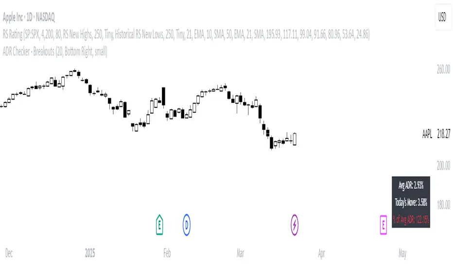
🧠 Example Use Case:
Imagine you're watching a classic VCP setup or flat base breakout. The stock breaks out on volume—but when you check this indicator, you see:
Today’s Move: 7.2%
Avg ADR: 5.3%
% of ADR: 135% 🟥
This tells you the stock is already well beyond its average daily range. While it may continue higher, odds now favor a consolidation, shakeout, or pullback. This is your cue to wait for a better entry or pass entirely.
On the flip side, if the breakout just started and the % of ADR is still under 50%, you have confirmation that there’s room to run — giving you more confidence to enter early.
⚙️ Fully Customizable:
Choose position on screen (top/bottom left/right)
Customize text color, background, and size
🔧 Install This Tool and:
✅ Stop chasing extended moves
✅ Add discipline to your entries
✅ Improve your breakout win rate
Perfect for VCP, CANSLIM, and BREAKOUT traders who want a clean, edge-enhancing visual guide.
Celestial Pair Spread Hello friends, after a very long time!
Today, I tried to put into code an idea that came to my mind spontaneously and suddenly.
Note :
This script is experimental and improvable.
I haven't had a chance to try it yet.
TIMEFRAME : 1D (Daily Bars)
CELESTIAL SPREAD
The spread moves in a very limited area and is consistent within itself, especially on days far from the end of the contract.
That's why there is a reassuring sky atmosphere. That's why this name was given completely improvised.
Basic logic of the script
We enter the name of the CME Futures contract we want to enter:
Ex : CL1! , ES1! , ZC1! , NQ1!
The script creates us a pair trade parity divided into secondary contracts.
Example : ES1!/ES2!
What is pair trading?
I will explain briefly here.
For users who are wondering:
www.investopedia.com
Let's get back to our topic.
Now we have created a parity that does not actually exist.
This parity is the manifestation of the relative movements of two contracts.
When the parity rises, ES1! increased,ES2! has fallen.
In the opposite case, We can say: ES1! Contract has been dropped ES2! has increased.
Pair trading is generally a trade that needs to be kept in mind from time to time.
It is a method preferred by professionals who can process very quickly.
Market risk is minimal, but since 2 contracts are purchased, more money is paid and very low percentage profits are made.
It is very expensive to do pair trading, especially with oil and its derivatives and interest security derivatives.
The contract we are considering has micros. (small-item contracts tied to the same value)
So when we switch to our broker MES1!/MES2! We will trade.
For all CME futures :
www.cmegroup.com
Anyway, let's continue:
The script created the parity showing its relationship with the next contract and plotted it as bars.
Celestial bands are just like Bollinger bands, but they consist of 3 bands based on percentage changes rather than standard deviation.
The middle band is obtained from moving averages.
The upper and lower bands are the middle band subjected to a threshold value.
The threshold value can be changed.
0.15 percent was charged for this script.
CAUTION :
As can be seen in the example below;
The most important thing is not to make any transactions when the contract switch dates are approaching.
Therefore, it is recommended to use it just below the main chart.
The blue bars in the parity are
Values that outside the upper and lower threshold values are colored blue.
For this condition
Alerts has been added.
Don't forget to add alert and edit.
MAIN PURPOSE
It is aimed to start a pair trade when such conditions come and to quickly close the trades when the parity basis reaches the value.
OTHER IMPORTANT POINTS
Other issues are broker related issues.
Difference between initial margins and maintanence margins of contracts (between 1! and 2!)
It shouldn't be too high.
The commission should not be too high.
Leverage must be high because the profit percentage is very low.
To calculate leverage you must divide your contract size by the relevant margin requirement.
Sample margin requirement table:
www.interactivebrokers.com
RISKS
It is an experimental and intellectual script,
the risk of contract price differences (maybe it will not leave a profit except for very extreme values)
I remind you of the quickness risk that comes from a two-legged trade.
Alerts definitely synchronized with an audible alert sent to a smartphone as an e-mail notification and displayed on the locked screen for quick action.
Best regards!

Overextension Oscillator [by DanielM]The Overextension Oscillator is an indicator that detects when a market move has extended significantly beyond its typical range, signaling potential areas for a correction or reversal. Unlike traditional oscillators that rely on fixed overbought/oversold levels, this tool dynamically adjusts its thresholds based on historical swing high and swing low movements.
By analyzing all swing points on the chart, the indicator determines the expected range of price movements and identifies when the price extends beyond normal levels. Since every asset has different price behavior and volatility, swing lengths may vary from asset to asset, ensuring that overextension is measured relative to each market's historical price behavior.
How It Works
1️⃣ Swing Detection & Data Collection
The indicator scans all available swing highs and swing lows on the chart to gather a complete dataset of past price fluctuations.
It records the percentage differences between swings to determine how much price typically moves in a given market.
2️⃣ Overextension Calculation
Using the stored swing data, the indicator calculates:
Average Swing Difference – Measures the average percentage difference between swings.
Average Move Percentage – Determines the typical magnitude of price moves within a trend cycle.
These values are used to create dynamic overextension thresholds that adjust based on historical data.
3️⃣ Price Distance & Overextension Measurement
The indicator calculates the distance between the current price and the closest historical swing point. If this distance exceeds the predefined threshold based on past swings, the move is considered overextended. The greater the deviation, the higher the probability of a pullback or short-term reversal.
4️⃣ Buy/Sell Signal Generation
A Buy signal is generated when the price has dropped below an overextended threshold relative to a past swing low.
A Sell signal is generated when the price has risen beyond an overextended threshold relative to a past swing high.
These signals indicate that the price has reached a level where it historically tends to slow down or reverse.

Accurate Bollinger Bands mcbw_ [True Volatility Distribution]The Bollinger Bands have become a very important technical tool for discretionary and algorithmic traders alike over the last decades. It was designed to give traders an edge on the markets by setting probabilistic values to different levels of volatility. However, some of the assumptions that go into its calculations make it unusable for traders who want to get a correct understanding of the volatility that the bands are trying to be used for. Let's go through what the Bollinger Bands are said to show, how their calculations work, the problems in the calculations, and how the current indicator I am presenting today fixes these.
--> If you just want to know how the settings work then skip straight to the end or click on the little (i) symbol next to the values in the indicator settings window when its on your chart <--
--------------------------- What Are Bollinger Bands ---------------------------
The Bollinger Bands were formed in the 1980's, a time when many retail traders interacted with their symbols via physically printed charts and computer memory for personal computer memory was measured in Kb (about a factor of 1 million smaller than today). Bollinger Bands are designed to help a trader or algorithm see the likelihood of price expanding outside of its typical range, the further the lines are from the current price implies the less often they will get hit. With a hands on understanding many strategies use these levels for designated levels of breakout trades or to assist in defining price ranges.
--------------------------- How Bollinger Bands Work ---------------------------
The calculations that go into Bollinger Bands are rather simple. There is a moving average that centers the indicator and an equidistant top band and bottom band are drawn at a fixed width away. The moving average is just a typical moving average (or common variant) that tracks the price action, while the distance to the top and bottom bands is a direct function of recent price volatility. The way that the distance to the bands is calculated is inspired by formulas from statistics. The standard deviation is taken from the candles that go into the moving average and then this is multiplied by a user defined value to set the bands position, I will call this value 'the multiple'. When discussing Bollinger Bands, that trading community at large normally discusses 'the multiple' as a multiplier of the standard deviation as it applies to a normal distribution (gaußian probability). On a normal distribution the number of standard deviations away (which trades directly use as 'the multiple') you are directly corresponds to how likely/unlikely something is to happen:
1 standard deviation equals 68.3%, meaning that the price should stay inside the 1 standard deviation 68.3% of the time and be outside of it 31.7% of the time;
2 standard deviation equals 95.5%, meaning that the price should stay inside the 2 standard deviation 95.5% of the time and be outside of it 4.5% of the time;
3 standard deviation equals 99.7%, meaning that the price should stay inside the 3 standard deviation 99.7% of the time and be outside of it 0.3% of the time.
Therefore when traders set 'the multiple' to 2, they interpret this as meaning that price will not reach there 95.5% of the time.
---------------- The Problem With The Math of Bollinger Bands ----------------
In and of themselves the Bollinger Bands are a great tool, but they have become misconstrued with some incorrect sense of statistical meaning, when they should really just be taken at face value without any further interpretation or implication.
In order to explain this it is going to get a bit technical so I will give a little math background and try to simplify things. First let's review some statistics topics (distributions, percentiles, standard deviations) and then with that understanding explore the incorrect logic of how Bollinger Bands have been interpreted/employed.
---------------- Quick Stats Review ----------------
.
(If you are comfortable with statistics feel free to skip ahead to the next section)
.
-------- I: Probability distributions --------
When you have a lot of data it is helpful to see how many times different results appear in your dataset. To visualize this people use "histograms", which just shows how many times each element appears in the dataset by stacking each of the same elements on top of each other to form a graph. You may be familiar with the bell curve (also called the "normal distribution", which we will be calling it by). The normal distribution histogram looks like a big hump around zero and then drops off super quickly the further you get from it. This shape (the bell curve) is very nice because it has a lot of very nifty mathematical properties and seems to show up in nature all the time. Since it pops up in so many places, society has developed many different shortcuts related to it that speed up all kinds of calculations, including the shortcut that 1 standard deviation = 68.3%, 2 standard deviations = 95.5%, and 3 standard deviations = 99.7% (these only apply to the normal distribution). Despite how handy the normal distribution is and all the shortcuts we have for it are, and how much it shows up in the natural world, there is nothing that forces your specific dataset to look like it. In fact, your data can actually have any possible shape. As we will explore later, economic and financial datasets *rarely* follow the normal distribution.
-------- II: Percentiles --------
After you have made the histogram of your dataset you have built the "probability distribution" of your own dataset that is specific to all the data you have collected. There is a whole complicated framework for how to accurately calculate percentiles but we will dramatically simplify it for our use. The 'percentile' in our case is just the number of data points we are away from the "middle" of the data set (normally just 0). Lets say I took the difference of the daily close of a symbol for the last two weeks, green candles would be positive and red would be negative. In this example my dataset of day by day closing price difference is:
week 1:
week 2:
sorting all of these value into a single dataset I have:
I can separate the positive and negative returns and explore their distributions separately:
negative return distribution =
positive return distribution =
Taking the 25th% percentile of these would just be taking the value that is 25% towards the end of the end of these returns. Or akin the 100%th percentile would just be taking the vale that is 100% at the end of those:
negative return distribution (50%) = -5
positive return distribution (50%) = +4
negative return distribution (100%) = -10
positive return distribution (100%) = +20
Or instead of separating the positive and negative returns we can also look at all of the differences in the daily close as just pure price movement and not account for the direction, in this case we would pool all of the data together by ignoring the negative signs of the negative reruns
combined return distribution =
In this case the 50%th and 100%th percentile of the combined return distribution would be:
combined return distribution (50%) = 4
combined return distribution (100%) = 10
Sometimes taking the positive and negative distributions separately is better than pooling them into a combined distribution for some purposes. Other times the combined distribution is better.
Most financial data has very different distributions for negative returns and positive returns. This is encapsulated in sayings like "Price takes the stairs up and the elevator down".
-------- III: Standard Deviation --------
The formula for the standard deviation (refereed to here by its shorthand 'STDEV') can be intimidating, but going through each of its elements will illuminate what it does. The formula for STDEV is equal to:
square root ( (sum ) / N )
Going back the the dataset that you might have, the variables in the formula above are:
'mean' is the average of your entire dataset
'x' is just representative of a single point in your dataset (one point at a time)
'N' is the total number of things in your dataset.
Going back to the STDEV formula above we can see how each part of it works. Starting with the '(x - mean)' part. What this does is it takes every single point of the dataset and measure how far away it is from the mean of the entire dataset. Taking this value to the power of two: '(x - mean) ^ 2', means that points that are very far away from the dataset mean get 'penalized' twice as much. Points that are very close to the dataset mean are not impacted as much. In practice, this would mean that if your dataset had a bunch of values that were in a wide range but always stayed in that range, this value ('(x - mean) ^ 2') would end up being small. On the other hand, if your dataset was full of the exact same number, but had a couple outliers very far away, this would have a much larger value since the square par of '(x - mean) ^ 2' make them grow massive. Now including the sum part of 'sum ', this just adds up all the of the squared distanced from the dataset mean. Then this is divided by the number of values in the dataset ('N'), and then the square root of that value is taken.
There is nothing inherently special or definitive about the STDEV formula, it is just a tool with extremely widespread use and adoption. As we saw here, all the STDEV formula is really doing is measuring the intensity of the outliers.
--------------------------- Flaws of Bollinger Bands ---------------------------
The largest problem with Bollinger Bands is the assumption that price has a normal distribution. This is assumption is massively incorrect for many reasons that I will try to encapsulate into two points:
Price return do not follow a normal distribution, every single symbol on every single timeframe has is own unique distribution that is specific to only itself. Therefore all the tools, shortcuts, and ideas that we use for normal distributions do not apply to price returns, and since they do not apply here they should not be used. A more general approach is needed that allows each specific symbol on every specific timeframe to be treated uniquely.
The distributions of price returns on the positive and negative side are almost never the same. A more general approach is needed that allows positive and negative returns to be calculated separately.
In addition to the issues of the normal distribution assumption, the standard deviation formula (as shown above in the quick stats review) is essentially just a tame measurement of outliers (a more aggressive form of outlier measurement might be taking the differences to the power of 3 rather than 2). Despite this being a bit of a philosophical question, does the measurement of outlier intensity as defined by the STDEV formula really measure what we want to know as traders when we're experiencing volatility? Or would adjustments to that formula better reflect what we *experience* as volatility when we are actively trading? This is an open ended question that I will leave here, but I wanted to pose this question because it is a key part of what how the Bollinger Bands work that we all assume as a given.
Circling back on the normal distribution assumption, the standard deviation formula used in the calculation of the bands only encompasses the deviation of the candles that go into the moving average and have no knowledge of the historical price action. Therefore the level of the bands may not really reflect how the price action behaves over a longer period of time.
------------ Delivering Factually Accurate Data That Traders Need------------
In light of the problems identified above, this indicator fixes all of these issue and delivers statistically correct information that discretionary and algorithmic traders can use, with truly accurate probabilities. It takes the price action of the last 2,000 candles and builds a huge dataset of distributions that you can directly select your percentiles from. It also allows you to have the positive and negative distributions calculated separately, or if you would like, you can pool all of them together in a combined distribution. In addition to this, there is a wide selection of moving averages directly available in the indicator to choose from.
Hedge funds, quant shops, algo prop firms, and advanced mechanical groups all employ the true return distributions in their work. Now you have access to the same type of data with this indicator, wherein it's doing all the lifting for you.
------------------------------ Indicator Settings ------------------------------
.
---- Moving average ----
Select the type of moving average you would like and its length
---- Bands ----
The percentiles that you enter here will be pulled directly from the return distribution of the last 2,000 candles. With the typical Bollinger Bands, traders would select 2 standard deviations and incorrectly think that the levels it highlights are the 95.5% levels. Now, if you want the true 95.5% level, you can just enter 95.5 into the percentile value here. Each of the three available bands takes the true percentile you enter here.
---- Separate Positive & Negative Distributions----
If this box is checked the positive and negative distributions are treated indecently, completely separate from each other. You will see that the width of the top and bottom bands will be different for each of the percentiles you enter.
If this box is unchecked then all the negative and positive distributions are pooled together. You will notice that the width of the top and bottom bands will be the exact same.
---- Distribution Size ----
This is the number of candles that the price return is calculated over. EG: to collect the price return over the last 33 candles, the difference of price from now to 33 candles ago is calculated for the last 2,000 candles, to build a return distribution of 2000 points of price differences over 33 candles.
NEGATIVE NUMBERS(<0) == exact number of candles to include;
EG: setting this value to -20 will always collect volatility distributions of 20 candles
POSITIVE NUMBERS(>0) == number of candles to include as a multiple of the Moving Average Length value set above;
EG: if the Moving Average Length value is set to 22, setting this value to 2 will use the last 22*2 = 44 candles for the collection of volatility distributions
MORE candles being include will generally make the bands WIDER and their size will change SLOWER over time.
I wish you focus, dedication, and earnest success on your journey.
Happy trading :)

RSI Divergence + Sweep + Signal + Alerts Toolkit [TrendX_]The RSI Toolkit is a powerful set of tools designed to enhance the functionality of the traditional Relative Strength Index (RSI) indicator. By integrating advanced features such as Moving Averages, Divergences, and Sweeps, it helps traders identify key market dynamics, potential reversals, and newly-approach trading stragies.
The toolkit expands on standard RSI usage by incorporating features from smart money concepts (Just try to be creative 🤣 Hope you like it), providing a deeper understanding of momentum, liquidity sweeps, and trend reversals. It is suitable for RSI traders who want to make more informed and effective trading decisions.
💎 FEATURES
RSI Moving Average
The RSI Moving Average (RSI MA) is the moving average of the RSI itself. It can be customized to use various types of moving averages, including Simple Moving Average (SMA), Exponential Moving Average (EMA), Relative Moving Average (RMA), and Volume-Weighted Moving Average (VWMA).
The RSI MA smooths out the RSI fluctuations, making it easier to identify trends and crossovers. It helps traders spot momentum shifts and potential entry/exit points by observing when the RSI crosses above or below its moving average.
RSI Divergence
RSI Divergence identifies discrepancies between price action and RSI momentum. There are two types of divergences: Regular Divergence - Indicates a potential trend reversal; Hidden Divergence - Suggests the continuation of the current trend.
Divergence is a critical signal for spotting weakness or strength in a trend. Regular divergence highlights potential trend reversals, while hidden divergence confirms trend continuation, offering traders valuable insights into market momentum and possible trade setups.
RSI Sweep
RSI Sweep detects moments when the RSI removes liquidity from a trend structure by sweeping above or below the price at key momentum level crossing. These sweeps are overlaid on the RSI chart for easier visualized.
RSI Sweeps are significant because they indicate potential turning points in the market. When RSI sweeps occur: In an uptrend - they suggest buyers' momentum has peaked, possibly leading to a reversal; In a downtrend - they indicate sellers’ momentum has peaked, also hinting at a reversal.
(Note: This feature incorporates Liquidity Sweep concepts from Smart Money Concepts into RSI analysis, helping RSI traders identify areas where liquidity has been removed, which often precedes a trend reversal)
🔎 BREAKDOWN
RSI Moving Average
How MA created: The RSI value is calculated first using the standard RSI formula. The MA is then applied to the RSI values using the trader’s chosen type of MA (SMA, EMA, RMA, or VWMA). The flexibility to choose the type of MA allows traders to adjust the smoothing effect based on their trading style.
Why use MA: RSI by itself can be noisy and difficult to interpret in volatile markets. Applying moving average would provide a smoother, more reliable view of RSI trends.
RSI Divergence
How Regular Divergence created: Regular Divergence is detected when price forms HIGHER highs while RSI forms LOWER highs (bearish divergence) or when price forms LOWER lows while RSI forms HIGHER lows (bullish divergence).
How Hidden Divergence created: Hidden Divergence is identified when price forms HIGHER lows while RSI forms LOWER lows (bullish hidden divergence) or when price forms LOWER highs while RSI forms HIGHER highs (bearish hidden divergence).
Why use Divergence: Divergences provide early warning signals of a potential trend change. Regular divergence helps traders anticipate reversals, while hidden divergence supports trend continuation, enabling traders to align their trades with market momentum.
RSI Sweep
How Sweep created: Trend Structure Shift are identified based on the RSI crossing key momentum level of 50. To track these sweeps, the indicator pinpoints moments when liquidity is removed from the Trend Structure Shift. This is a direct application of Liquidity Sweep concepts used in Smart Money theories, adapted to RSI.
Why use Sweep: RSI Sweeps are created to help traders detect potential trend reversals. By identifying areas where momentum has exhausted during a certain trend direction, the indicator highlights opportunities for traders to enter trades early in a reversal or continuation phase.
⚙️ USAGES
Divergence + Sweep
This is an example of combining Devergence & Sweep in BTCUSDT (1 hour)
Wait for a divergence (regular or hidden) to form on the RSI. After the divergence is complete, look for a sweep to occur. A potential entry might be formed at the end of the sweep.
Divergences indicate a potential trend change, but confirmation is required to ensure the setup is valid. The RSI Sweep provides that confirmation by signaling a liquidity event, increasing the likelihood of a successful trade.
Sweep + MA Cross
This is an example of combining Devergence & Sweep in BTCUSDT (1 hour)
Wait for an RSI Sweep to form then a potential entry might be formed when the RSI crosses its MA.
The RSI Sweep highlights a potential turning point in the market. The MA cross serves as additional confirmation that momentum has shifted, providing a more reliable and more potential entry signal for trend continuations.
DISCLAIMER
This indicator is not financial advice, it can only help traders make better decisions. There are many factors and uncertainties that can affect the outcome of any endeavor, and no one can guarantee or predict with certainty what will occur. Therefore, one should always exercise caution and judgment when making decisions based on past performance.
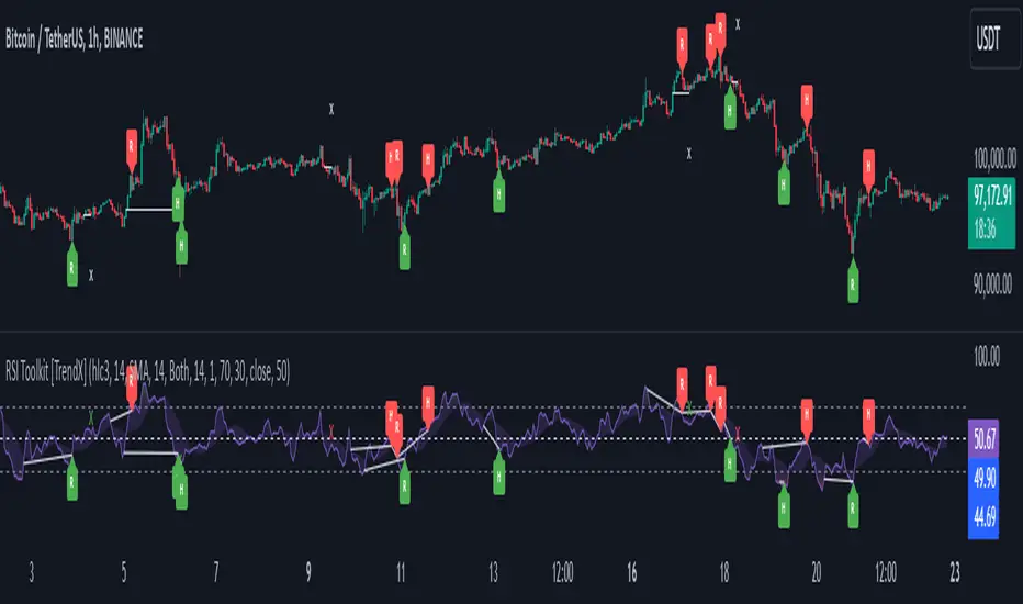
Drawdown from All-Time High (Line)This Pine Script is a **Drawdown Indicator from All-Time High** for TradingView. It calculates and plots the percentage drawdown from the highest price the asset has ever reached (the all-time high). Here's a breakdown of what this script does:
### Description:
- **Drawdown Calculation**:
- The drawdown is calculated as the difference between the current price (`close`) and the all-time high, divided by the all-time high, and multiplied by 100 to express it as a percentage.
- If the current price is higher than the previous all-time high, the all-time high is updated to the current price.
- **All-Time High Tracking**:
- The script tracks the highest price (`allTimeHigh`) that the asset has ever reached. Each time a new high is reached, the `allTimeHigh` value is updated.
- **Line Plot**:
- The drawdown percentage is then plotted as a line on the chart, with a color of **blue** for easy visualization.
- The line shows how much the price has dropped relative to its all-time high.
- **Zero Line**:
- A horizontal line is added at the **0%** level to act as a reference point, which is helpful to identify when the asset has fully recovered to its all-time high.
### Key Features:
- **Track Drawdown**: The indicator helps visualize how far the current price has fallen from its highest point, which is useful for understanding the depth of losses (drawdowns) during a period.
- **Update All-Time High**: The indicator automatically updates the all-time high whenever a new high is detected.
- **Visual Reference**: The 0% horizontal line provides a clear indication of when the asset is at its all-time high, and the drawdown is at 0%.
### How it Works:
- If the current price surpasses the all-time high, the script will reset the all-time high to the new price.
- The drawdown percentage is calculated from the current price relative to this all-time high, and it is displayed as a line on the chart.
### Visuals:
- **Drawdown Line**: Plots the percentage of the drawdown, which is the drop from the all-time high.
- **Zero Line**: A dotted horizontal line at 0% marks the level of the all-time high.
This indicator is valuable for understanding the extent of price corrections and potential recoveries relative to the historical peak of the asset. It is especially useful for traders and investors who want to assess the risk of drawdowns in relation to the highest price achieved by the asset.

ImbalancesThis Pine Script is a trading indicator designed to identify imbalances in the market, specifically on candlestick charts. An imbalance refers to situations where there is a significant difference between buyers and sellers, which can create gaps or areas of inefficiency in the price. These imbalances often act as zones where price may return to "fill" or correct these inefficiencies.
1. Identifying Imbalances
The script analyzes candlestick patterns to detect imbalances based on the relationship between the highs, lows, and closes of consecutive candles. Specifically, it looks for:
Top Imbalances (Bearish): Areas where selling pressure has dominated, causing inefficiencies in the price. These are represented by patterns like multiple consecutive bearish candles or bearish gaps.
Bottom Imbalances (Bullish): Areas where buying pressure has dominated, leading to bullish gaps or inefficiencies.
When an imbalance is detected, the script highlights the area using visual boxes on the chart.
2. Visual Representation
The indicator uses colored boxes to show imbalances directly on the chart:
Top (Bearish) Imbalances: Highlighted using shades of red.
Bottom (Bullish) Imbalances: Highlighted using shades of green.
The boxes are further categorized into three states based on their level of mitigation:
Unmitigated: The imbalance has not been "filled" by price yet.
Partially Mitigated: Price has entered the imbalance zone but not completely filled it.
Fully Mitigated: Price has completely filled the imbalance zone.
3. Mitigation Logic
The concept of mitigation refers to the price revisiting an imbalance zone to correct the inefficiency:
If price fully or partially revisits an imbalance zone, the box's color changes to indicate the mitigation level (e.g., from unmitigated to partially/fully mitigated).
Fully mitigated boxes may be removed or recolored, depending on user preferences.
4. User Customization
The script provides several inputs to customize its behavior:
Enable or disable top and bottom imbalance detection.
Color settings: Users can define different colors for unmitigated, partially mitigated, and fully mitigated imbalances.
Mitigation display options: Users can choose whether to show fully mitigated imbalances on the chart or remove them.
5. Key Calculations
Imbalance Size: The size of the imbalance is calculated as the price difference between a candle's high and low across the relevant pattern.
Pattern Detection: The script checks for specific candlestick patterns (e.g., three consecutive bearish candles) to identify potential imbalances.
6. Practical Use Case
This indicator is useful for traders who:
Rely on supply and demand zones for their trading strategies.
Look for areas where price is likely to return (retesting unmitigated imbalances can signal potential trade setups).
Want to visually track market inefficiencies over time.
In Summary
The "Imbalances" indicator highlights and tracks price inefficiencies on candlestick charts. It marks zones where buying or selling pressure was dominant, and it dynamically updates these zones based on price action to indicate their mitigation status. This tool is particularly helpful for traders who use price action and market structure in their strategies.

Heiken Ashi MTF Monitor - Better Formula - EMA, AMA, KAFA, T3Heiken Ashi MTF Monitor - Better Formula - EMA, AMA, KAFA, T3
This indicator is based on the works of Loxx & Smart_Money-Trader, without their initial codes, none of this will be possible.
This Pine Script indicator provides a multi-timeframe (MTF) analysis of Heiken Ashi trends, designed to enhance the traditional Heiken Ashi method with advanced smoothing techniques such as the Exponential Moving Average (EMA), Adaptive Moving Average (AMA), Kaufman’s Adaptive Moving Average (KAMA), and the Triple Exponential Moving Average (T3). The indicator offers a flexible approach to identify bullish, bearish, and neutral trends across six customizable timeframes and various Heiken Ashi calculation methods.
Key Features:
Multi-Timeframe (MTF) Support: The indicator allows you to monitor trends across six timeframes (e.g., 2-hour, 4-hour, daily, weekly, monthly), giving a holistic view of market conditions at different scales.
Heiken Ashi Calculation Methods: Choose between traditional Heiken Ashi or an enhanced "Better HA" method for more refined trend analysis.
Smoothing Options: Apply different smoothing techniques, including EMA, T3, KAMA, or AMA, to the Heiken Ashi values for smoother, more reliable trend signals.
Non-Repaint Option: This feature ensures that the values do not repaint after the bar closes, providing a more reliable historical view.
Customizable Plotting: The indicator offers full customization of which timeframes to display and whether to show labels for each timeframe.
Inputs and Settings:
Timeframe Inputs:
Users can set up to six different timeframes, ranging from intraday (2-hour, 4-hour) to higher timeframes (daily, weekly, monthly).
Timeframes can be enabled or disabled individually for each analysis.
Label Visibility:
Labels indicating the trend direction (bullish, bearish, neutral) can be shown for each timeframe. This helps with clarity when monitoring multiple timeframes simultaneously.
Smoothing Options:
EMA: Exponential Moving Average for standard smoothing.
AMA: Adaptive Moving Average, which adapts its smoothing based on market volatility.
KAMA: Kaufman’s Adaptive Moving Average, which adjusts its sensitivity to price fluctuations.
T3: Triple Exponential Moving Average, providing a smoother and more responsive moving average.
None: No smoothing applied (for raw Heiken Ashi calculations).
Non-Repaint Setting:
Enabling this ensures the trend values do not change after the bar closes, offering a stable historical view of trends.
Core Functions:
Heiken Ashi Calculations:
Traditional HA: The classic Heiken Ashi calculation is used here, where each bar's open, close, high, and low are computed based on the average price of the previous bar.
Better HA: A refined calculation method, where the raw Heiken Ashi close is adjusted by considering the price range. This smoother value is then optionally processed through a moving average function for further smoothing.
Heiken Ashi Trend Calculation:
Based on the selected Heiken Ashi method (Traditional or Better HA), the indicator checks whether the trend is bullish (upward movement), bearish (downward movement), or neutral (sideways movement).
For the "Better HA" method, the trend determination uses the difference between the smoothed Heiken Ashi close and open.
Moving Averages:
The moving averages applied to the Heiken Ashi values are configurable:
EMA: Standard smoothing with an exponential weighting.
T3: A triple exponential smoothing technique that provides a smoother moving average.
KAMA: An adaptive smoothing technique that adjusts to market noise.
AMA: An adaptive moving average that reacts to market volatility, making it more flexible.
None: For raw, unsmoothed Heiken Ashi data.
Trend Detection:
The indicator evaluates the direction of the trend for each timeframe and assigns a color-coded value (bearish, bullish, or neutral).
The trend values are plotted as circles, and their color reflects the detected trend: red for bearish, green for bullish, and white for neutral.
Multi-Timeframe (MTF) Support:
The indicator can be used to analyze up to six different timeframes simultaneously.
The trend for each timeframe is calculated and displayed as circles on the chart.
Users can enable or disable individual timeframes, allowing for a customizable view based on which timeframes they are interested in monitoring.
Plotting:
The indicator plots circles at specific levels based on the detected trend (Level 1 for the 2-hour timeframe, Level 2 for the 4-hour timeframe, etc.). The size and color of these circles represent the trend direction.
These plotted values provide a quick visual reference for trend direction across multiple timeframes.
Usage:
Trend Confirmation: By monitoring trends across multiple timeframes, traders can use this indicator to confirm trends and avoid false signals.
Customizable Timeframe Analysis: Traders can focus on shorter timeframes for intraday trades or look at longer timeframes for a broader market perspective.
Smoothing for Clarity: By applying various moving average techniques, traders can reduce noise and get a clearer view of the trend.
Non-Repainting: The non-repaint option ensures the indicator values remain consistent even after the bar closes, providing more reliable signals for backtesting or live trading.
This Heiken Ashi MTF Monitor indicator with better formulas and smoothing options is designed for traders who want to analyze trends across multiple timeframes while benefiting from advanced moving averages and more refined Heiken Ashi calculations. The customizable settings for smoothing, timeframe selection, and label visibility allow users to tailor the indicator to their specific needs and trading style.

WillStop Pro [tradeviZion]WillStop Pro : A Step-by-Step Guide for Beginners to Master Trend Trading
Welcome to an in-depth guide to the WillStop Pro indicator. This article will walk you through the key features, how to use them effectively, and how this tool can help you navigate the markets confidently. WillStop Pro is based on principles established by Larry Williams, a well-known figure in trading, and aims to help you manage trades more effectively without overcomplicating things.
This guide will help you understand the basics of the WillStop Pro indicator, how to interpret its signals, and how to use it step-by-step to manage risk and identify opportunities in your trading journey. We will also cover the underlying logic and calculations for advanced users interested in more details.
What is the WillStop Pro Indicator?
The WillStop Pro indicator is a user-friendly tool that helps traders establish stop levels dynamically. It helps you figure out optimal points to enter or exit trades, while managing risk effectively during changing market conditions. The indicator tracks trending markets and sets price levels as stops for ongoing trades, making it suitable both for deciding when to enter and exit trades.
The indicator is beginner-friendly because it simplifies complex calculations and presents the results visually. This allows traders to focus more on their decision-making process instead of spending time with complex analysis.
WillStop Pro adapts to different market conditions, whether you're trading stocks, forex, commodities, or cryptocurrencies. It adjusts stop levels dynamically based on current market momentum, providing a practical way to manage both risk and reward.
Another significant benefit of WillStop Pro is that it works well with other indicators. Beginners can use it on its own or combine it with other tools like moving averages or oscillators to form a comprehensive trading strategy. Whether you are trading daily or looking at longer-term trends, WillStop Pro helps you manage your trades effectively.
Key Features of WillStop Pro
Dynamic Stop Levels : WillStop Pro calculates real-time stop levels for both long (buy) and short (sell) positions. This helps you protect your profits and reduce risk. The stop levels adjust based on the current market environment, making them more adaptable compared to fixed stop levels.
Advanced Stop Settings : There are optional settings to make the stop calculations more advanced, which take into consideration previous price movements to refine where the stops should be placed. These settings provide more precise control over your trades.
Break Signals and Alerts : The indicator provides visual signals, like arrows, to show when a stop level has been broken. This makes it easier for you to identify possible reversals and understand when the market direction is changing.
Comprehensive Table Display : A small table on the chart shows the current trend, the stop level, and whether advanced mode is active. This simple display provides an overview of the market, making decision-making easier.
Based on Larry Williams' Methodology : WillStop Pro builds upon Larry Williams' ideas, which are designed to capture major market trends while managing risk effectively. It provides a systematic way to follow these strategies without requiring deep technical analysis skills.
How Are Stop Levels Calculated? (For Advanced Users)
The WillStop Pro indicator determines stop levels by evaluating highs, lows, and closing prices over a specific lookback period. It uses this information to identify key points that justify adjusting your stop level, and there are separate approaches for both long and short positions.
Below, we explain the mathematical logic behind the stop calculations, along with some code snippets to give advanced users a clearer understanding.
For Long Stops (buy positions): The indicator looks for the highest closing price within the lookback period and continues until it finds three valid bars that meet certain criteria. Stops are adjusted to skip bars that have consecutive upward closes to ensure that the stop is placed at a level that offers solid support. Specifically, the function iterates over recent bars to determine the highest closing value, and checks for specific conditions before finalizing the stop level. Here is an excerpt of the relevant code:
getTrueLow(idx) => math.min(low , close )
findStopLevels() =>
float highestClose = close
int highestCloseIndex = 0
for i = 0 to lookback
if close > highestClose
highestClose := close
highestCloseIndex := i
// Logic to adjust based on up close skipping
int longCount = 0
int longCurrentIndex = highestCloseIndex
while longCount < 3 and longCurrentIndex < 100
if not isInsideBar(longCurrentIndex)
longCount += 1
longCurrentIndex += 1
// Determine the lowest low for the stop level
float longStopLevel = high * 2
for i = searchIndex to highestCloseIndex
longStopLevel := math.min(longStopLevel, getTrueLow(i))
// Apply offset
longStopLevel := longStopLevel - (offsetTicks * tickSize)
In this code snippet, the function findStopLevels() calculates the long stop level by first identifying the highest close within the lookback period and then finding a suitable support level while skipping certain conditions, such as inside bars or consecutive upward closes. Finally, the user-defined offset ( offsetTicks ) is applied to determine the stop level.
For Short Stops (sell positions): Similarly, the indicator finds the lowest closing price within the lookback period and then identifies three bars that fit the conditions for a short stop. It avoids using bars with consecutive down closes to help find a more robust resistance level. Here's a relevant code snippet:
getTrueHigh(idx) => math.max(high , close )
findStopLevels() =>
float lowestClose = close
int lowestCloseIndex = 0
for i = 0 to lookback
if close < lowestClose
lowestClose := close
lowestCloseIndex := i
// Logic to adjust based on down close skipping
int shortCount = 0
int shortCurrentIndex = lowestCloseIndex
while shortCount < 3 and shortCurrentIndex < 100
if not isInsideBar(shortCurrentIndex)
shortCount += 1
shortCurrentIndex += 1
// Determine the highest high for the stop level
float shortStopLevel = 0
for i = searchIndex to lowestCloseIndex
shortStopLevel := math.max(shortStopLevel, getTrueHigh(i))
// Apply offset
shortStopLevel := shortStopLevel + (offsetTicks * tickSize)
Here, findStopLevels() calculates the short stop level by finding the lowest closing price within the lookback period. It then determines the highest value that acts as a resistance level, excluding bars that do not fit certain criteria.
Volume Confirmation for Alert Accuracy : To further enhance the stop level accuracy, volume is used as a confirmation filter. The average volume (volAvg) is calculated over a 20-period moving average, and alerts are only generated if the volume exceeds a defined threshold (volMultiplier). This ensures that price movements are significant enough to consider as meaningful signals.
volAvg = ta.sma(volume, 20)
isVolumeConfirmed() =>
result = requireVolumeConfirmation ? volume > (volAvg * volMultiplier) : true
result
This additional logic ensures that stop level breaks or adjustments are not triggered during periods of low trading activity, thus enhancing the reliability of the generated signals.
These calculations are at the core of WillStop Pro's ability to determine dynamic stop levels that respond effectively to market movements, helping traders manage risk by placing stops at levels that make sense given historical price and volume data.
How to Identify Opportunities with WillStop Pro
WillStop Pro provides various signals that help you decide when to enter or exit a trade:
When a Stop Level is Broken: If a stop level (support for long positions or resistance for short positions) is broken, it may indicate a reversal. WillStop Pro visually plots arrows whenever a stop level is breached, making it easy for you to see where changes might occur. This feature helps traders identify momentum shifts quickly.
Support and Resistance Levels: The indicator plots support and resistance levels, which show key zones to watch for opportunities. These levels often act as psychological barriers in the market, where price action may either reverse or stall temporarily.
Dynamic State Management: The indicator shifts between long and short states based on price action, providing real-time feedback. This helps traders stick to their trading plan without second-guessing the market.
A major advantage of WillStop Pro is that it responds well to changing market conditions. By identifying when key support or resistance levels break, it allows you to adjust your strategies and react to new opportunities accordingly. Whether the market is trending strongly or staying within a range, WillStop Pro provides valuable information to help guide your trades.
Setting Up Alerts
Alerts are an important feature in trading, especially when you can’t be in front of your charts all the time. WillStop Pro has been enhanced to include flexible alert settings to help you stay on top of your trades without constantly monitoring the charts.
Enable Alerts: There is a master switch to enable or disable all alerts. This way, you can control whether you want to be notified of events at any time.
Alert Frequency: Choose between receiving alerts Once Per Bar or Once Per Bar Close . This helps you manage the frequency of alerts and decide if you need real-time updates or want confirmation after a bar closes.
Break Alerts: These alerts notify you when a stop level has been broken. This can help you catch potential reversals or trading opportunities as soon as they happen.
Strong Break Alerts: Alerts are available for strong breaks, which occur when the price breaks stop levels with confirmation based on additional price, volume, and momentum criteria. These alerts help identify significant shifts in the market.
Level Change Alerts: These alerts tell you whenever a new stop level is calculated, keeping you updated about changes in market dynamics. You can set a Minimum Level Change % to ensure that alerts are only triggered when the stop level changes significantly.
Require Volume Confirmation: You can opt to receive alerts only if the volume is above a certain threshold. This confirmation helps reduce false signals by ensuring that significant price changes are backed by increased trading activity.
Volume Multiplier: The volume multiplier allows you to set a minimum volume requirement that must be met for an alert to trigger. This ensures that alerts are triggered only when there is sufficient trading interest.
Here is a part of the updated alert logic that has been implemented in the indicator:
// Alert on break conditions
if alertsEnabled
if alertOnBreaks
if longStopBroken and isVolumeConfirmed()
alert(createAlertMessage("Support Break - Short Signal", useAdvancedStops), alertFreq)
if shortStopBroken and isVolumeConfirmed()
alert(createAlertMessage("Resistance Break - Long Signal", useAdvancedStops), alertFreq)
// Strong break alerts
if alertOnStrongBreaks
if longStopBroken and isStrongBreak(false)
alert(createAlertMessage("Strong Support Break - Short Signal", useAdvancedStops), alertFreq)
if shortStopBroken and isStrongBreak(true)
alert(createAlertMessage("Strong Resistance Break - Long Signal", useAdvancedStops), alertFreq)
// Level change alerts
if alertOnLevelChanges and isSignificantChange() and isVolumeConfirmed()
alert(createAlertMessage("Significant Level Change", useAdvancedStops), alertFreq)
Setting alerts allows you to react to market changes without having to watch the charts constantly. Alerts are particularly helpful if you have other responsibilities and can’t be actively monitoring your trades all day.
Understanding the Table Display
The WillStop Pro indicator provides a status table that gives an overview of the current market state. Here’s what the table shows:
Indicator Status: The table indicates whether the indicator is in a LONG or SHORT state. This helps you quickly understand the market trend.
Stop Level: The active stop level is shown, whether it is acting as support (long) or resistance (short). This is important for knowing where to set your protective stops.
Mode: The table also displays whether the advanced calculation mode is being used. This keeps you informed about how stop levels are being calculated and why they are positioned where they are.
Empowering Messages: The table also includes motivational messages that rotate periodically, such as 'Trade with Clarity, Stop with Precision' and 'Let Winners Run, Cut Losses Short.' These messages are designed to keep you focused, motivated, and disciplined during your trading journey.
The table is simple and easy to follow, helping you maintain discipline in your trading plan. By having all the essential information in one place, the table reduces the need to make quick, emotional decisions and promotes more thoughtful analysis.
Tips for Using WillStop Pro Effectively
Here are some practical ways to make the most of the WillStop Pro indicator:
Start with Default Settings: If you’re new to the indicator, start with the default settings. This will give you an idea of how stop levels are determined and how they adjust to different markets.
Experiment with Advanced Settings: Once you are comfortable, try using the advanced stop settings to see how they refine the stop levels. This can be useful in certain market conditions to improve accuracy.
Use Alerts to Stay Updated: Set up alerts for when a stop level is broken or when new levels are calculated. This helps you take action without constantly watching the chart. Swing traders may find alerts especially helpful for monitoring longer-term moves.
Monitor the Status Table: Keep an eye on the status table to understand the current market condition. Whether the indicator is in a LONG or SHORT state can help you make more informed decisions.
Focus on Risk Management: WillStop Pro is designed to help you manage risk by dynamically adjusting stop levels. Make sure you are using these levels to protect your trades, especially during strong trends or volatile periods.
Acknowledging Larry Williams' Influence
WillStop Pro is inspired by the work of Larry Williams, who described the approach as one of his best trading techniques. His method aims to ride major market trends while reducing the risk of giving back gains during corrections. WillStop Pro builds upon this approach, adding features like advanced stop settings and visual alerts that make it easier to apply in modern markets.
By using WillStop Pro, you are essentially leveraging a well-established trading strategy with additional tools that help improve its effectiveness. The indicator is designed to provide a reliable way to manage trades, stay on top of market conditions, and reduce emotional decision-making.
Conclusion: Why WillStop Pro is Great for Beginners and Advanced Users
The WillStop Pro is a powerful yet easy-to-use tool that helps traders ride trends while managing risk during market corrections. It can be used both for entering and exiting trades, and its visual features make it accessible for those who are new to trading, while the underlying logic appeals to advanced users seeking greater control and understanding.
WillStop Pro is more than just a tool for setting stops. It is a comprehensive solution for managing trades, with features like dynamic stop levels, customizable alerts, and an easy-to-understand status table. This combination of simplicity and advanced features makes it suitable for beginners as well as more experienced traders.
We hope this guide helps you get started with WillStop Pro and improves your trading confidence. Remember to start with the basics, explore the advanced features, and set alerts to stay informed without getting overwhelmed. Whether you’re just beginning or want to simplify your strategy, WillStop Pro is a valuable tool to have in your trading arsenal.
Trading can be challenging, but the right tools make it more manageable. WillStop Pro helps you keep track of market movements, identify opportunities, and manage risk effectively. Give it a try and see how it can improve your trading decisions and help you navigate the markets more efficiently.
By incorporating WillStop Pro into your strategy, you are following a systematic approach that has been refined over time. It’s designed to help you make sense of the markets, plan your trades, and manage your risks with greater clarity and confidence.
Note: Always practice proper risk management and thoroughly test the indicator to ensure it aligns with your trading strategy. Past performance is not indicative of future results.
Trade smarter with TradeVizion—unlock your trading potential today!

Supertrend Scanner on ChartThis Indicator is Used to scan 10 stock on chart.
Supertrend is widely used indicator on tradingview. So we have used the originals indicator codes of supertrend by tradingview here. Background color has been changed as per supertrend trrend.
Problem : Sometime trader wants to track multiple stocks supertrend at a time. Mostly those stock are of same sector. To track all the stocks of same sector in one chart , trader has to open multiple charts for that.
Solution : This indicator pointout where other stocks has changed the trend. Like if you see "SBIN" written in GEREEN at bottom of the candle , that means on that particular candle SBIN supertrend has changed to positive. Similarly if you see "KOTAK" written in RED at top of the candle the means supertrend has changed to Negative on that particular candle. Its so easy to trace 10 stock on same chart which stocks labelling.
How to use :
When you trade on any index , then apply all the index constituents stock on this indicator. When Index changes the trend and that change in trend is confirmed by other constituents ( like 7/10 confirmed ) then that is confirmed trend. If all the constituents are on same direction than that's the confirmed trend.
Disclamer : This indicator is for education purpose , for any profit or loss , we are not responsible. Trade on your own risk.

Price Action Smart Money Concepts [BigBeluga]THE SMART MONEY CONCEPTS Toolkit
The Smart Money Concepts [ BigBeluga ] is a comprehensive toolkit built around the principles of "smart money" behavior, which refers to the actions and strategies of institutional investors.
The Smart Money Concepts Toolkit brings together a suite of advanced indicators that are all interconnected and built around a unified concept: understanding and trading like institutional investors, or "smart money." These indicators are not just randomly chosen tools; they are features of a single overarching framework, which is why having them all in one place creates such a powerful system.
This all-in-one toolkit provides the user with a unique experience by automating most of the basic and advanced concepts on the chart, saving them time and improving their trading ideas.
Real-time market structure analysis simplifies complex trends by pinpointing key support, resistance, and breakout levels.
Advanced order block analysis leverages detailed volume data to pinpoint high-demand zones, revealing internal market sentiment and predicting potential reversals. This analysis utilizes bid/ask zones to provide supply/demand insights, empowering informed trading decisions.
Imbalance Concepts (FVG and Breakers) allows traders to identify potential market weaknesses and areas where price might be attracted to fill the gap, creating opportunities for entry and exit.
Swing failure patterns help traders identify potential entry points and rejection zones based on price swings.
Liquidity Concepts, our advanced liquidity algorithm, pinpoints high-impact events, allowing you to predict market shifts, strong price reactions, and potential stop-loss hunting zones. This gives traders an edge to make informed trading decisions based on liquidity dynamics.
🔵 FEATURES
The indicator has quite a lot of features that are provided below:
Swing market structure
Internal market structure
Mapping structure
Adjustable market structure
Strong/Weak H&L
Sweep
Volumetric Order block / Breakers
Fair Value Gaps / Breakers (multi-timeframe)
Swing Failure Patterns (multi-timeframe)
Deviation area
Equal H&L
Liquidity Prints
Buyside & Sellside
Sweep Area
Highs and Lows (multi-timeframe)
🔵 BASIC DEMONSTRATION OF ALL FEATURES
1. MARKET STRUCTURE
The preceding image illustrates the market structure functionality within the Smart Money Concepts indicator.
➤ Solid lines: These represent the core indicator's internal structure, forming the foundation for most other components. They visually depict the overall market direction and identify major reversal points marked by significant price movements (denoted as 'x').
➤ Internal Structure: These represent an alternative internal structure with the potential to drive more rapid market shifts. This is particularly relevant when a significant gap exists in the established swing structure, specifically between the Break of Structure (BOS) and the most recent Change of High/Low (CHoCH). Identifying these formations can offer opportunities for quicker entries and potential short-term reversals.
➤ Sweeps (x): These signify potential turning points in the market where liquidity is removed from the structure. This suggests a possible trend reversal and presents crucial entry opportunities. Sweeps are identified within both swing and internal structures, providing valuable insights for informed trading decisions.
➤ Mapping structure: A tool that automatically identifies and connects significant price highs and lows, creating a zig-zag pattern. It visualizes market structure, highlights trends, support/resistance levels, and potential breakouts. Helps traders quickly grasp price action patterns and make informed decisions.
➤ Color-coded candles based on market structure: These colors visually represent the underlying market structure, making it easier for traders to quickly identify trends.
➤ Extreme H&L: It visualizes market structure with extreme high and lows, which gives perspective for macro Market Structure.
2. VOLUMETRIC ORDER BLOCKS
Order blocks are specific areas on a financial chart where significant buying or selling activity has occurred. These are not just simple zones; they contain valuable information about market dynamics. Within each of these order blocks, volume bars represent the actual buying and selling activity that took place. These volume bars offer deeper insights into the strength of the order block by showing how much buying or selling power is concentrated in that specific zone.
Additionally, these order blocks can be transformed into Breaker Blocks. When an order block fails—meaning the price breaks through this zone without reversing—it becomes a breaker block. Breaker blocks are particularly useful for trading breakouts, as they signal that the market has shifted beyond a previously established zone, offering opportunities for traders to enter in the direction of the breakout.
Here's a breakdown:
➤ Bear Order Blocks (Red): These are zones where a lot of selling happened. Traders see these areas as places where sellers were strong, pushing the price down. When the price returns to these zones, it might face resistance and drop again.
➤ Bull Order Blocks (Green): These are zones where a lot of buying happened. Traders see these areas as places where buyers were strong, pushing the price up. When the price returns to these zones, it might find support and rise again.
These Order Blocks help traders identify potential areas for entering or exiting trades based on past market activity. The volume bars inside blocks show the amount of trading activity that occurred in these blocks, giving an idea of the strength of buying or selling pressure.
➤ Breaker Block: When an order block fails, meaning the price breaks through this zone without reversing, it becomes a breaker block. This indicates a significant shift in market liquidity and structure.
➤ A bearish breaker block occurs after a bullish order block fails. This typically happens when there's an upward trend, and a certain level that was expected to support the market's rise instead gives way, leading to a sharp decline. This decline indicates that sellers have overcome the buyers, absorbing liquidity and shifting the sentiment from bullish to bearish.
Conversely, a bullish breaker block is formed from the failure of a bearish order block. In a downtrend, when a level that was expected to act as resistance is breached, and the price shoots up, it signifies that buyers have taken control, overpowering the sellers.
3. FAIR VALUE GAPS:
A fair value gap (FVG), also referred to as an imbalance, is an essential concept in Smart Money trading. It highlights the supply and demand dynamics. This gap arises when there's a notable difference between the volume of buy and sell orders. FVGs can be found across various asset classes, including forex, commodities, stocks, and cryptocurrencies.
FVGs in this toolkit have the ability to detect raids of FVG which helps to identify potential price reversals.
Mitigation option helps to change from what source FVGs will be identified: Close, Wicks or AVG.
4. SWING FAILURE PATTERN (SFP):
The Swing Failure Pattern is a liquidity engineering pattern, generally used to fill large orders. This means, the SFP generally occurs when larger players push the price into liquidity pockets with the sole objective of filling their own positions.
SFP is a technical analysis tool designed to identify potential market reversals. It works by detecting instances where the price briefly breaks a previous high or low but fails to maintain that breakout, quickly reversing direction.
How it works:
Pattern Detection: The indicator scans for price movements that breach recent highs or lows.
Reversal Confirmation: If the price quickly reverses after breaching these levels, it's identified as an SFP.
➤ SFP Display:
Bullish SFP: Marked with a green symbol when price drops below a recent low before reversing upwards.
Bearish SFP: Marked with a red symbol when price rises above a recent high before reversing downwards.
➤ Deviation Levels: After detecting an SFP, the indicator projects white lines showing potential price deviation:
For bullish SFPs, the deviation line appears above the current price.
For bearish SFPs, the deviation line appears below the current price.
These deviation levels can serve as a potential trading opportunity or areas where the reversal might lose momentum.
With Volume Threshold and Filtering of SFP traders can adjust their trading style:
Volume Threshold: This setting allows traders to filter SFPs based on the volume of the reversal candle. By setting a higher volume threshold, traders can focus on potentially more significant reversals that are backed by higher trading activity.
SFP Filtering: This feature enables traders to filter SFP detection. It includes parameters such as:
5. LIQUIDITY CONCEPTS:
➤ Equal Lows (EQL) and Equal Highs (EQH) are important concepts in liquidity-based trading.
EQL: A series of two or more swing lows that occur at approximately the same price level.
EQH: A series of two or more swing highs that occur at approximately the same price level.
EQLs and EQHs are seen as potential liquidity pools where a large number of stop loss orders or limit orders may be clustered. They can be used as potential reverse points for trades.
This multi-period feature allows traders to select less and more significant EQL and EQH:
➤ Liquidity wicks:
Liquidity wicks are a minor representation of a stop-loss hunt during the retracement of a pivot point:
➤ Buy and Sell side liquidity:
The buy side liquidity represents a concentration of potential buy orders below the current price level. When price moves into this area, it can lead to increased buying pressure due to the execution of these orders.
The sell side liquidity indicates a pool of potential sell orders below the current price level. Price movement into this area can result in increased selling pressure as these orders are executed.
➤ Sweep Liquidation Zones:
Sweep Liquidation Zones are crucial for understanding market structure and potential future price movements. They provide insights into areas where significant market participants have been forced out of their positions, potentially setting up new trading opportunities.
🔵 USAGE & EXAMPLES
The core principle behind the success of this toolkit lies in identifying "confluence." This refers to the convergence of multiple trading indicators all signaling the same information at a specific point or area. By seeking such alignment, traders can significantly enhance the likelihood of successful trades.
MS + OBs
The chart illustrates a highly bullish setup where the price is rejecting from a bullish order block (POC), while simultaneously forming a bullish Swing Failure Pattern (SFP). This occurs after an internal structure change, marked by a bullish Change of Character (CHoCH). The price broke through a bearish order block, transforming it into a breaker block, further confirming the bullish momentum.
The combination of these elements—bullish order blocks, SFP, and CHoCH—creates a powerful bullish signal, reinforcing the potential for upward movement in the market.
SFP + Bear OB
This chart above displays a bearish setup with a high probability of a price move lower. The price is currently rejecting from a bear order block, which represents a key resistance area where significant selling pressure has previously occurred. A Swing Failure Pattern (SFP) has also formed near this bear order block, indicating that the price briefly attempted to break above a recent high but failed to sustain that upward movement. This failure suggests that buyers are losing momentum, and the market could be preparing for a move to the downside.
Additionally, we can toggle on the Deviation Area in the SFP section to highlight potential levels where price deviation might occur. These deviation areas represent zones where the price is likely to react after the Swing Failure Pattern:
BUY – SELL sides + EQL
The chart showcases a bullish setup with a high probability of price breaking out of the current sell-side resistance level. The market structure indicates a formation of Equal Lows (EQL), which often suggests a build-up of liquidity that could drive the price higher.
The presence of strong buy-side pressure (69%), indicated by the green zone at the bottom, reinforces this bullish outlook. This area represents a key support zone where buyers are outpacing sellers, providing the foundation for a potential upward breakout.
EQL + Bull ChoCh
This chart illustrates a potential bullish setup, driven by the formation of Equal Lows (EQL) followed by a bullish Change of Character (CHoCH). The presence of Equal Lows often signals a liquidity build-up, which can lead to a reversal when combined with additional bullish signals.
Liquidity grab + Bull ChoCh + FVGs
This chart demonstrates a strong bullish scenario, where several important market dynamics are at play. The price begins its upward momentum from Liquidity grab following a bullish Change of Character (CHoCH), signaling the transition from a bearish phase to a bullish one.
As the price progresses, it performs liquidity grabs, which serve to gather the necessary fuel for further movement. These liquidity grabs often occur before significant price surges, as large market participants exploit these areas to accumulate positions before pushing the price higher.
The chart also highlights a market imbalance area, showing strong momentum as the price moves swiftly through this zone.
In this examples, we see how the combination of multiple “smart money” tools helps identify a potential trade opportunities. This is just one of the many scenarios that traders can spot using this toolkit. Other combinations—such as order blocks, liquidity grabs, fair value gaps, and Swing Failure Patterns (SFPs)—can also be layered on top of these concepts to further refine your trading strategy.
🔵 SETTINGS
Window: limit calculation period
Swing: limit drawing function
Mapping structure: show structural points
Algorithmic Logic: (Extreme-Adjusted) Use max high/low or pivot point calculation
Algorithmic loopback: pivot point look back
Show Last: Amount of Order block to display
Hide Overlap: hide overlapping order blocks
Construction: Size of the order blocks
Fair value gaps: Choose between normal FVG or Breaker FVG
Mitigation: (close - wick - avg) point to mitigate the order block/imbalance
SFP lookback: find a higher / lower point to improve accuracy
Threshold: remove less relevant SFP
Equal H&L: (short-mid-long term) display longer term
Liquidity Prints: Shows wicks of candles where liquidity was grabbed
Sweep Area: Identify Sweep Liquidation areas
By combining these indicators in one toolkit, traders are equipped with a comprehensive suite of tools that address every angle of the Smart Money Concept. Instead of relying on disparate tools spread across various platforms, having them integrated into a single, cohesive system allows traders to easily see confluence and make more informed trading decisions.

ADR Study [TFO]This indicator is focused on the Average Daily Range (ADR), with the goal of collecting data to show how often price reaches/closes through these levels, as well as a look at historical moves that reached ADR and at similar times of day to study how price moved for the remainder of the session.
The ADR here (blue line) is calculated using the difference between a day's highest and lowest points. If our ADR length is 5, then we are taking this difference from the last 5 days and averaging them together. At the following day's open, we take half of this average and plot it above and below the daily opening price to place theoretical limits on how far price may move according to the lookback period. The triangles indicate when price has reached ADR (either +ADR or -ADR), and alerts can be created for these events.
The Scale Factor is an optional parameter to scale the ADR by a certain amount. If set to 2 for example, then the ADR would be 2x the average daily range. This value will be reflected in the statistics options so that users can see how different values affect the outcomes.
Show Table will display data collected on how often price reaches these levels, and how often price closes through them, for each day of the week. By default, these are colored as blue and red, respectively. From the following chart of NQ1!, we can see for example that on Mondays, price reached +ADR 38% of the time and closed through it 23% of the time. Note that the statistics for closing through the ADR levels are derived from all instances, not just those that reached ADR.
Show Sample Sizes will display how many instances were collected for all given sets of data. Referring to the same example of NQ1!, we can see that this particular chart has collected data from 109 Mondays. From those Mondays, 41 reached +ADR (38%, verifying our initial claim) and 25 closed through it (23%). This is important to understand the scope of the data that we're working with, as percentages can be misleading for smaller sample sizes.
Show Histogram will plot the same exact data as the table, just in a histogram form to visually emphasize the differences on a day-by-day basis. On this chart of RTY1!, we can see for example from the top histogram that on Wednesdays, 40% reached +ADR and only 22% closed through it. Similarly if we look at the bottom histogram, we can see that Wednesdays reached -ADR 46% of the time and closed through it only 28% of the time.
We can also use Show Sample Sizes to display the same information that would be in the table, showing how many instances were collected for each event. In this case we can see that we observed 175 Fridays, where 76 reached +ADR (43%) and 44 closed above it (25%).
Show Historical Moves is an interesting feature of this script. When enabled, if price has reached +/- ADR in the current session, the indicator will plot the evolution of the close prices from all past sessions that reached +/- ADR to see how they traded for the remainder of the session. These calculations are made with respect to the ADR range at the time that price traded through these levels.
Historical Proximity (Bars) allows the user to observe historical moves where price reached ADR within this many bars of the current session (assuming price has reached an ADR level in the current session). In the above chart, this is set to 1000 so that we can observe each and every instance where price reached an ADR level. However, we can refine this a bit more.
By limiting the Historical Proximity to something like 20, we are only considering historical moves that reached ADR within 20 bars of todays +ADR reach (9:50 am EST, noted by the blue triangle up). We can enable Show Average Move to display the average move by the filtered dataset, and Match +/-ADR to only observe moves inline with the current day's price action (in this case, only moves that reached +ADR, since price has not reached -ADR).
We can add one more filter to this data with the setting Only Show Days That: closed through ADR; closed within ADR; or either. The option either is what you see above, as we are considering both days that closed through ADR and days that closed within it (note that in this case, closing within ADR simply means that price reached +ADR and closed the day below it, and vice versa for -ADR; this does not mean that price must have closed in between +ADR and -ADR). If we set this to only show instances that closed within ADR, we see the following data.
Alternatively, we can choose to Only Show Days That closed through ADR, where we would see the following data. In this case, the average move very much resembles the price action that occurred on this particular day. This is in no way guaranteed, but it makes an interesting case for how we could use this data in our analysis by observing similar, historical price action.
Please note that this data will change over time on a rolling basis due to TradingView's bar lookback, and that for this same reason, lower timeframes will yield less data than larger timeframes.
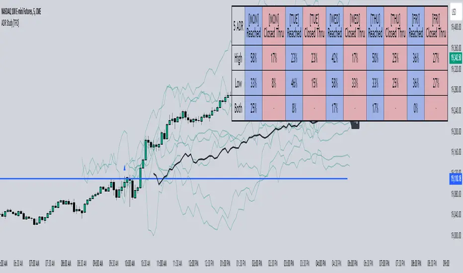
Intellect_city - World Cycle - Ath - Timeframe 1D and 1WIndicator Overview
The Pi Cycle Top Indicator has historically been effective in picking out the timing of market cycle highs within 3 days.
It uses the 111 day moving average (111DMA) and a newly created multiple of the 350 day moving average, the 350DMA x 2.
Note: The multiple is of the price values of the 350DMA, not the number of days.
For the past three market cycles, when the 111DMA moves up and crosses the 350DMA x 2 we see that it coincides with the price of Bitcoin peaking.
It is also interesting to note that 350 / 111 is 3.153, which is very close to Pi = 3.142. In fact, it is the closest we can get to Pi when dividing 350 by another whole number.
It once again demonstrates the cyclical nature of Bitcoin price action over long time frames. However, in this instance, it does so with a high degree of accuracy over Bitcoin's adoption phase of growth.
Bitcoin Price Prediction Using This Tool
The Pi Cycle Top Indicator forecasts the cycle top of Bitcoin’s market cycles. It attempts to predict the point where Bitcoin price will peak before pulling back. It does this on major high time frames and has picked the absolute tops of Bitcoin’s major price moves throughout most of its history.
How It Can Be Used
Pi Cycle Top is useful to indicate when the market is very overheated. So overheated that the shorter-term moving average, which is the 111-day moving average, has reached an x2 multiple of the 350-day moving average. Historically, it has proved advantageous to sell Bitcoin around this time in Bitcoin's price cycles.
It is also worth noting that this indicator has worked during Bitcoin's adoption growth phase, the first 15 years or so of Bitcoin's life. With the launch of Bitcoin ETF's and Bitcoin's increased integration into the global financial system, this indicator may cease to be relevant at some point in this new market structure.

Momentum Alligator 4h Bitcoin StrategyOverview
The Momentum Alligator 4h Bitcoin Strategy is a trend-following trading system that operates on dual time frames. It utilizes the 1D Williams Alligator indicator to identify the prevailing major price trend and seeks trading opportunities on the 4-hour (4h) time frame when the momentum is turning up. The strategy is designed to close trades if the trend fails to develop or holding position if price continues increasing without any significant correction. Note that this strategy is specifically tailored for the 4-hour time frame.
Unique Features
2-layers market noise filtering system: Trades are only initiated in the direction of the 1D trend, determined by the Williams Alligator indicator. This higher time frame confirmation filters out minor trade signals, focusing on more substantial opportunities. At the same time, strategy has additional filter on 4h time frame with Awesome Oscillator which is showing the current price momentum.
Flexible Risk Management: The strategy exclusively opens long positions, resulting in fewer trades during bear markets. It incorporates a dynamic stop-loss mechanism, which can either follow the jaw line of the 4h Alligator or a user-defined fixed stop-loss. This flexibility helps manage risk and avoid non-trending markets.
Methodology
The strategy initiates a long position when the d-line of Stochastic RSI crosses up it's k-line. It means that there is a high probability that price momentum reversed from down to up. To avoid overtrading in potentially choppy markets, it skips the next two trades following a winning trade, anticipating sideways movement after a significant price surge.
This strategy has two layers trades filtering system: 4h and 1D time frames. The first one is awesome oscillator. It shall be increasing and value has to be higher than it's 5-period SMA. This is an additional confirmation that long trade is opened in the direction of the current momentum. As it was mentioned above, all entry signals are validated against the 1D Williams Alligator indicator. A trade is only opened if the price is above all three lines of the 1D Alligator, ensuring alignment with the major trend.
A trade is closed if the price hits the 4h jaw line of the Alligator or reaches the user-defined stop-loss level.
Risk Management
The strategy employs a combined approach to risk management:
It allows positions to ride the trend as long as the price continues to move favorably, aiming to capture significant price movements. It features a user-defined stop-loss parameter to mitigate risks based on individual risk tolerance. By default, this stop-loss is set to a 2% drop from the entry point, but it can be adjusted according to the trader's preferences.
Justification of Methodology
This strategy leverages Stochastic RSI on 4h time frame to open long trade when momentum started reversing to the upside. On the one hand, Stochastic RSI is one of the most sensitive indicator, which allows to react fast on the potential trend reversal. On the other hand, this indicator can be too sensitive and provide a lot of false trend changing signals. To eliminate this weakness we use two-layers trades filtering system.
The first layer is the 4h Awesome oscillator. This is less sensitive momentum indicator. Usually it starts increasing when price has already passed significant distance from the actual reversal point. The strategy opens long trade only is Awesome oscillator is increasing and above it's 5-period SMA. This approach increases the probability to filter the false signals during the choppy market or if the reversal is false.
The second layer filter is the Williams Alligator indicator on 1D time frame. The 1D Alligator serves as a filter for identifying the primary trend and increases probability to avoid the trades with low potential because trading against major trend usually is more risky. It's much better to catch the trend continuation than local bounce.
Last but not least feature of this strategy is close trades condition. It uses the flexible approach. First of all, user can set up the fixed stop-loss according to his own risk-tolerance, by default this value is 2% of price movement. It restricts the potential loss at the moment when trade has just been opened. Moreover strategy utilizes the 4h Williams Alligator's jaw line to exit the trade. If price fell below it trade is closed. This approach helps to not keep open trade if trend is not developing and hold it if price continues going up.
Backtest Results:
Operating window: Date range of backtests is 2021.01.01 - 2024.05.01. It is chosen to let the strategy to close all opened positions.
Commission and Slippage: Includes a standard Binance commission of 0.1% and accounts for possible slippage over 5 ticks.
Initial capital: 10000 USDT
Percent of capital used in every trade: 50%
Maximum Single Position Loss: -3.04%
Maximum Single Profit: +29.67%
Net Profit: +6228.01 USDT (+62.28%)
Total Trades: 118 (24.58% win rate)
Profit Factor: 1.71
Maximum Accumulated Loss: 1527.69 USDT (-11.52%)
Average Profit per Trade: 52.78 USDT (+0.89%)
Average Trade Duration: 60 hours
These results are obtained with realistic parameters representing trading conditions observed at major exchanges such as Binance and with realistic trading portfolio usage parameters.
How to Use:
Add the script to favorites for easy access.
Apply to the 4h timeframe desired chart (optimal performance observed on the BTC/USDT).
Configure settings using the dropdown choice list in the built-in menu.
Set up alerts to automate strategy positions through web hook with the text: {{strategy.order.alert_message}}
Disclaimer:
Educational and informational tool reflecting Skyrex commitment to informed trading. Past performance does not guarantee future results. Test strategies in a simulated environment before live implementation
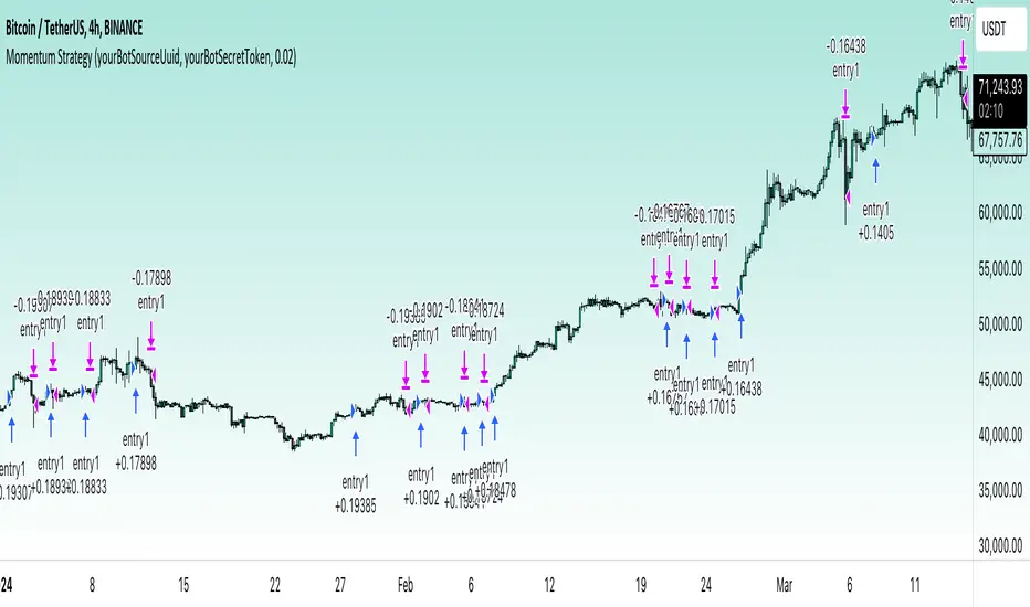
Bitcoin Momentum StrategyThis is a very simple long-only strategy I've used since December 2022 to manage my Bitcoin position.
I'm sharing it as an open-source script for other traders to learn from the code and adapt it to their liking if they find the system concept interesting.
General Overview
Always do your own research and backtesting - this script is not intended to be traded blindly (no script should be) and I've done limited testing on other markets beyond Ethereum and BTC, it's just a template to tweak and play with and make into one's own.
The results shown in the strategy tester are from Bitcoin's inception so as to get a large sample size of trades, and potential returns have diminished significantly as BTC has grown to become a mega cap asset, but the script includes a date filter for backtesting and it has still performed solidly in recent years (speaking from personal experience using it myself - DYOR with the date filter).
The main advantage of this system in my opinion is in limiting the max drawdown significantly versus buy & hodl. Theoretically much better returns can be made by just holding, but that's also a good way to lose 70%+ of your capital in the inevitable bear markets (also speaking from experience).
In saying all of that, the future is fundamentally unknowable and past results in no way guarantee future performance.
System Concept:
Capture as much Bitcoin upside volatility as possible while side-stepping downside volatility as quickly as possible.
The system uses a simple but clever momentum-style trailing stop technique I learned from one of my trading mentors who uses this approach on momentum/trend-following stock market systems.
Basically, the system "ratchets" up the stop-loss to be much tighter during high bearish volatility to protect open profits from downside moves, but loosens the stop loss during sustained bullish momentum to let the position ride.
It is invested most of the time, unless BTC is trading below its 20-week EMA in which case it stays in cash/USDT to avoid holding through bear markets. It only trades one position (no pyramiding) and does not trade short, but can easily be tweaked to do whatever you like if you know what you're doing in Pine.
Default parameters:
HTF: Weekly Chart
EMA: 20-Period
ATR: 5-period
Bar Lookback: 7
Entry Rule #1:
Bitcoin's current price must be trading above its higher-timeframe EMA (Weekly 20 EMA).
Entry Rule #2:
Bitcoin must not be in 'caution' condition (no large bearish volatility swings recently).
Enter at next bar's open if conditions are met and we are not already involved in a trade.
"Caution" Condition:
Defined as true if BTC's recent 7-bar swing high minus current bar's low is > 1.5x ATR, or Daily close < Daily 20-EMA.
Trailing Stop:
Stop is trailed 1 ATR from recent swing high, or 20% of ATR if in caution condition (ie. 0.2 ATR).
Exit on next bar open upon a close below stop loss.
I typically use a limit order to open & exit trades as close to the open price as possible to reduce slippage, but the strategy script uses market orders.
I've never had any issues getting filled on limit orders close to the market price with BTC on the Daily timeframe, but if the exchange has relatively low slippage I've found market orders work fine too without much impact on the results particularly since BTC has consistently remained above $20k and highly liquid.
Cost of Trading:
The script uses no leverage and a default total round-trip commission of 0.3% which is what I pay on my exchange based on their tier structure, but this can vary widely from exchange to exchange and higher commission fees will have a significantly negative impact on realized gains so make sure to always input the correct theoretical commission cost when backtesting any script.
Static slippage is difficult to estimate in the strategy tester given the wide range of prices & liquidity BTC has experienced over the years and it largely depends on position size, I set it to 150 points per buy or sell as BTC is currently very liquid on the exchange I trade and I use limit orders where possible to enter/exit positions as close as possible to the market's open price as it significantly limits my slippage.
But again, this can vary a lot from exchange to exchange (for better or worse) and if BTC volatility is high at the time of execution this can have a negative impact on slippage and therefore real performance, so make sure to adjust it according to your exchange's tendencies.
Tax considerations should also be made based on short-term trade frequency if crypto profits are treated as a CGT event in your region.
Summary:
A simple, but effective and fairly robust system that achieves the goals I set for it.
From my preliminary testing it appears it may also work on altcoins but it might need a bit of tweaking/loosening with the trailing stop distance as the default parameters are designed to work with Bitcoin which obviously behaves very differently to smaller cap assets.
Good luck out there!
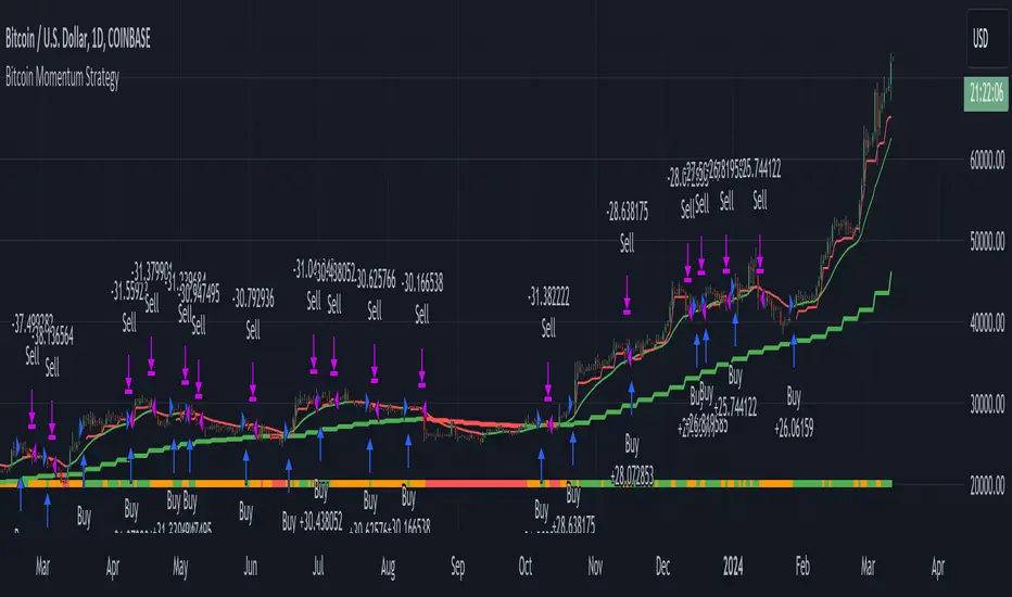
Support and Resistance ZoneSupport and Resistance Zone Indicator :
Introduction :
The purpose of this indicator is to identify the chart symbol's main supports and resistances. It displays these key zones, which are very important psychological points for traders. Since support and resistance are not very precise levels, the indicator displays them as zones.
Pivots :
Pivots are a key concept in identifying support and resistance. The indicator uses two types of pivot:
Pivot high : This is a high point that has not been reached by a user-defined number of candles on either the left and right of this candle. The " left pivot leg " is the number of candles before this pivot point that have not reached the realized high, and the " right pivot leg " is the number of candles after this pivot point that have not reached this high. If these two conditions are met, the pivot point is considered a turning point, and resistance is probably the cause.
Pivot low : This is a low point that has not been reached by a user-defined number of candles on either the left or right. The " left pivot leg " is the number of candles before this pivot point that have not reached the candle low, and the " right pivot leg " is the number of candles after this pivot point that have not reached this low. If these two conditions are met, the pivot point is considered a turning point, and support is probably the cause.
Support/Resistance area :
If a pivot point has been identified, the indicator considers it a resistance if it's a pivot high, or a support if it's a pivot low. To define the support or resistance zone, we'll use the ATR (Average True Range), an indicator that measures asset volatility. We'll take the ATR of the candle for which the pivot was spotted, and use it as the width of the support or resistance zone. Thus the upper line of support/resistance is at pivot+atr/2 and the lower line is at pivot-atr/2 . The greater the volatility, the larger the zone.
New Support/Resistance :
If a new pivot has been identified, but the level of this pivot lies between the lower line and the upper line of the previous support or resistance, the indicator considers this to be the same support or resistance as before. In this case, no new support or resistance is created. The pivot must be outside the area of the previous support or resistance to be validated.
Anticipated Support/Resistance :
This indicator also allows early detection of support or resistance. To do this, the value of the right pivot legs will be shortened in order to find these areas more quickly. The support or resistance will then be considered anticipated and may disappear at any time if the high/low is reached. On the other hand, if the high/low is not reached, and a number of candles equal to the " Right Pivot Legs" parameter has elapsed since the detection of this anticipated support/resistance, it will be considered validated and will integrate the other supports/resistances of the chart.
Extended supports/resistances :
For a more optimal view, the indicator allows the user to choose the number of last support or resistance levels to be extended to the last candle. This must be specified in the indicator parameters.
Parameters :
Pivot Legs : Determine the left and right legs of the pivot i.e the number of candle before and after the pivot that doesn’t reach pivot point. The pivot is validated only if this two conditions are verified.
Extend Last Supports : Number of supports to extend to the last bar
Extend Last Resistances : Number of resistances to extend to the last bar
Show Support/Resistance Anticipated : If yes, will find anticipated support and resistance
Right Pivot Legs for Anticipation : Determine the right legs of pivots to find faster a support or a resistance.
Conclusion :
This indicator plot support and resistance zones based on pivot. The width of support and resistance zones are calculated with ATR. Possibility to find anticipated support and resistance in order to have more timeliness informations.
Enjoy the indicator and don’t forget to take the trade ;)