Signal Generator: HTF EMA Momentum + MACDSignal Generator: HTF EMA Momentum + MACD
What this script does
This indicator combines a higher-timeframe EMA trend filter with a MACD crossover on the chart’s timeframe. The goal is to make MACD signals more selective by checking whether they occur in the same direction as the broader trend.
How it works
- On the higher timeframe, two EMAs are calculated (short and long). Their difference is used as a simple momentum measure.
- On the chart timeframe, the MACD is calculated. Crossovers are then filtered with two conditions:
1.They must align with the higher-timeframe EMA trend.
2.They must occur beyond a small “zero band” threshold, with a minimum distance between MACD and signal lines.
- When both conditions are met, the script can plot BUY or SELL labels. ATR is used only to shift labels up or down for visibility.
Visuals and alerts
- Histogram bars show whether higher-timeframe EMA momentum is rising or falling.
- MACD main and signal lines are plotted with optional scaling.
- Dotted lines show the zero band region.
- Optional large BUY/SELL labels appear when conditions are confirmed on the previous bar.
- Alerts can be enabled for these signals; they trigger once per bar close.
Notes and limitations
- Higher-timeframe values are only confirmed once the higher-timeframe candle has closed.
- Scaling factors affect appearance only, not the logic.
- This is an open-source study intended as a learning and charting tool. It does not provide financial advice or guarantee performance.
Pesquisar nos scripts por "crossover债券是什么"

Tzotchev Trend Measure [EdgeTools]Are you still measuring trend strength with moving averages? Here is a better variant at scientific level:
Tzotchev Trend Measure: A Statistical Approach to Trend Following
The Tzotchev Trend Measure represents a sophisticated advancement in quantitative trend analysis, moving beyond traditional moving average-based indicators toward a statistically rigorous framework for measuring trend strength. This indicator implements the methodology developed by Tzotchev et al. (2015) in their seminal J.P. Morgan research paper "Designing robust trend-following system: Behind the scenes of trend-following," which introduced a probabilistic approach to trend measurement that has since become a cornerstone of institutional trading strategies.
Mathematical Foundation and Statistical Theory
The core innovation of the Tzotchev Trend Measure lies in its transformation of price momentum into a probability-based metric through the application of statistical hypothesis testing principles. The indicator employs the fundamental formula ST = 2 × Φ(√T × r̄T / σ̂T) - 1, where ST represents the trend strength score bounded between -1 and +1, Φ(x) denotes the normal cumulative distribution function, T represents the lookback period in trading days, r̄T is the average logarithmic return over the specified period, and σ̂T represents the estimated daily return volatility.
This formulation transforms what is essentially a t-statistic into a probabilistic trend measure, testing the null hypothesis that the mean return equals zero against the alternative hypothesis of non-zero mean return. The use of logarithmic returns rather than simple returns provides several statistical advantages, including symmetry properties where log(P₁/P₀) = -log(P₀/P₁), additivity characteristics that allow for proper compounding analysis, and improved validity of normal distribution assumptions that underpin the statistical framework.
The implementation utilizes the Abramowitz and Stegun (1964) approximation for the normal cumulative distribution function, achieving accuracy within ±1.5 × 10⁻⁷ for all input values. This approximation employs Horner's method for polynomial evaluation to ensure numerical stability, particularly important when processing large datasets or extreme market conditions.
Comparative Analysis with Traditional Trend Measurement Methods
The Tzotchev Trend Measure demonstrates significant theoretical and empirical advantages over conventional trend analysis techniques. Traditional moving average-based systems, including simple moving averages (SMA), exponential moving averages (EMA), and their derivatives such as MACD, suffer from several fundamental limitations that the Tzotchev methodology addresses systematically.
Moving average systems exhibit inherent lag bias, as documented by Kaufman (2013) in "Trading Systems and Methods," where he demonstrates that moving averages inevitably lag price movements by approximately half their period length. This lag creates delayed signal generation that reduces profitability in trending markets and increases false signal frequency during consolidation periods. In contrast, the Tzotchev measure eliminates lag bias by directly analyzing the statistical properties of return distributions rather than smoothing price levels.
The volatility normalization inherent in the Tzotchev formula addresses a critical weakness in traditional momentum indicators. As shown by Bollinger (2001) in "Bollinger on Bollinger Bands," momentum oscillators like RSI and Stochastic fail to account for changing volatility regimes, leading to inconsistent signal interpretation across different market conditions. The Tzotchev measure's incorporation of return volatility in the denominator ensures that trend strength assessments remain consistent regardless of the underlying volatility environment.
Empirical studies by Hurst, Ooi, and Pedersen (2013) in "Demystifying Managed Futures" demonstrate that traditional trend-following indicators suffer from significant drawdowns during whipsaw markets, with Sharpe ratios frequently below 0.5 during challenging periods. The authors attribute these poor performance characteristics to the binary nature of most trend signals and their inability to quantify signal confidence. The Tzotchev measure addresses this limitation by providing continuous probability-based outputs that allow for more sophisticated risk management and position sizing strategies.
The statistical foundation of the Tzotchev approach provides superior robustness compared to technical indicators that lack theoretical grounding. Fama and French (1988) in "Permanent and Temporary Components of Stock Prices" established that price movements contain both permanent and temporary components, with traditional moving averages unable to distinguish between these elements effectively. The Tzotchev methodology's hypothesis testing framework specifically tests for the presence of permanent trend components while filtering out temporary noise, providing a more theoretically sound approach to trend identification.
Research by Moskowitz, Ooi, and Pedersen (2012) in "Time Series Momentum in the Cross Section of Asset Returns" found that traditional momentum indicators exhibit significant variation in effectiveness across asset classes and time periods. Their study of multiple asset classes over decades revealed that simple price-based momentum measures often fail to capture persistent trends in fixed income and commodity markets. The Tzotchev measure's normalization by volatility and its probabilistic interpretation provide consistent performance across diverse asset classes, as demonstrated in the original J.P. Morgan research.
Comparative performance studies conducted by AQR Capital Management (Asness, Moskowitz, and Pedersen, 2013) in "Value and Momentum Everywhere" show that volatility-adjusted momentum measures significantly outperform traditional price momentum across international equity, bond, commodity, and currency markets. The study documents Sharpe ratio improvements of 0.2 to 0.4 when incorporating volatility normalization, consistent with the theoretical advantages of the Tzotchev approach.
The regime detection capabilities of the Tzotchev measure provide additional advantages over binary trend classification systems. Research by Ang and Bekaert (2002) in "Regime Switches in Interest Rates" demonstrates that financial markets exhibit distinct regime characteristics that traditional indicators fail to capture adequately. The Tzotchev measure's five-tier classification system (Strong Bull, Weak Bull, Neutral, Weak Bear, Strong Bear) provides more nuanced market state identification than simple trend/no-trend binary systems.
Statistical testing by Jegadeesh and Titman (2001) in "Profitability of Momentum Strategies" revealed that traditional momentum indicators suffer from significant parameter instability, with optimal lookback periods varying substantially across market conditions and asset classes. The Tzotchev measure's statistical framework provides more stable parameter selection through its grounding in hypothesis testing theory, reducing the need for frequent parameter optimization that can lead to overfitting.
Advanced Noise Filtering and Market Regime Detection
A significant enhancement over the original Tzotchev methodology is the incorporation of a multi-factor noise filtering system designed to reduce false signals during sideways market conditions. The filtering mechanism employs four distinct approaches: adaptive thresholding based on current market regime strength, volatility-based filtering utilizing ATR percentile analysis, trend strength confirmation through momentum alignment, and a comprehensive multi-factor approach that combines all methodologies.
The adaptive filtering system analyzes market microstructure through price change relative to average true range, calculates volatility percentiles over rolling windows, and assesses trend alignment across multiple timeframes using exponential moving averages of varying periods. This approach addresses one of the primary limitations identified in traditional trend-following systems, namely their tendency to generate excessive false signals during periods of low volatility or sideways price action.
The regime detection component classifies market conditions into five distinct categories: Strong Bull (ST > 0.3), Weak Bull (0.1 < ST ≤ 0.3), Neutral (-0.1 ≤ ST ≤ 0.1), Weak Bear (-0.3 ≤ ST < -0.1), and Strong Bear (ST < -0.3). This classification system provides traders with clear, quantitative definitions of market regimes that can inform position sizing, risk management, and strategy selection decisions.
Professional Implementation and Trading Applications
The indicator incorporates three distinct trading profiles designed to accommodate different investment approaches and risk tolerances. The Conservative profile employs longer lookback periods (63 days), higher signal thresholds (0.2), and reduced filter sensitivity (0.5) to minimize false signals and focus on major trend changes. The Balanced profile utilizes standard academic parameters with moderate settings across all dimensions. The Aggressive profile implements shorter lookback periods (14 days), lower signal thresholds (-0.1), and increased filter sensitivity (1.5) to capture shorter-term trend movements.
Signal generation occurs through threshold crossover analysis, where long signals are generated when the trend measure crosses above the specified threshold and short signals when it crosses below. The implementation includes sophisticated signal confirmation mechanisms that consider trend alignment across multiple timeframes and momentum strength percentiles to reduce the likelihood of false breakouts.
The alert system provides real-time notifications for trend threshold crossovers, strong regime changes, and signal generation events, with configurable frequency controls to prevent notification spam. Alert messages are standardized to ensure consistency across different market conditions and timeframes.
Performance Optimization and Computational Efficiency
The implementation incorporates several performance optimization features designed to handle large datasets efficiently. The maximum bars back parameter allows users to control historical calculation depth, with default settings optimized for most trading applications while providing flexibility for extended historical analysis. The system includes automatic performance monitoring that generates warnings when computational limits are approached.
Error handling mechanisms protect against division by zero conditions, infinite values, and other numerical instabilities that can occur during extreme market conditions. The finite value checking system ensures data integrity throughout the calculation process, with fallback mechanisms that maintain indicator functionality even when encountering corrupted or missing price data.
Timeframe validation provides warnings when the indicator is applied to unsuitable timeframes, as the Tzotchev methodology was specifically designed for daily and higher timeframe analysis. This validation helps prevent misapplication of the indicator in contexts where its statistical assumptions may not hold.
Visual Design and User Interface
The indicator features eight professional color schemes designed for different trading environments and user preferences. The EdgeTools theme provides an institutional blue and steel color palette suitable for professional trading environments. The Gold theme offers warm colors optimized for commodities trading. The Behavioral theme incorporates psychology-based color contrasts that align with behavioral finance principles. The Quant theme provides neutral colors suitable for analytical applications.
Additional specialized themes include Ocean, Fire, Matrix, and Arctic variations, each optimized for specific visual preferences and trading contexts. All color schemes include automatic dark and light mode optimization to ensure optimal readability across different chart backgrounds and trading platforms.
The information table provides real-time display of key metrics including current trend measure value, market regime classification, signal strength, Z-score, average returns, volatility measures, filter threshold levels, and filter effectiveness percentages. This comprehensive dashboard allows traders to monitor all relevant indicator components simultaneously.
Theoretical Implications and Research Context
The Tzotchev Trend Measure addresses several theoretical limitations inherent in traditional technical analysis approaches. Unlike moving average-based systems that rely on price level comparisons, this methodology grounds trend analysis in statistical hypothesis testing, providing a more robust theoretical foundation for trading decisions.
The probabilistic interpretation of trend strength offers significant advantages over binary trend classification systems. Rather than simply indicating whether a trend exists, the measure quantifies the statistical confidence level associated with the trend assessment, allowing for more nuanced risk management and position sizing decisions.
The incorporation of volatility normalization addresses the well-documented problem of volatility clustering in financial time series, ensuring that trend strength assessments remain consistent across different market volatility regimes. This normalization is particularly important for portfolio management applications where consistent risk metrics across different assets and time periods are essential.
Practical Applications and Trading Strategy Integration
The Tzotchev Trend Measure can be effectively integrated into various trading strategies and portfolio management frameworks. For trend-following strategies, the indicator provides clear entry and exit signals with quantified confidence levels. For mean reversion strategies, extreme readings can signal potential turning points. For portfolio allocation, the regime classification system can inform dynamic asset allocation decisions.
The indicator's statistical foundation makes it particularly suitable for quantitative trading strategies where systematic, rules-based approaches are preferred over discretionary decision-making. The standardized output range facilitates easy integration with position sizing algorithms and risk management systems.
Risk management applications benefit from the indicator's ability to quantify trend strength and provide early warning signals of potential trend changes. The multi-timeframe analysis capability allows for the construction of robust risk management frameworks that consider both short-term tactical and long-term strategic market conditions.
Implementation Guide and Parameter Configuration
The practical application of the Tzotchev Trend Measure requires careful parameter configuration to optimize performance for specific trading objectives and market conditions. This section provides comprehensive guidance for parameter selection and indicator customization.
Core Calculation Parameters
The Lookback Period parameter controls the statistical window used for trend calculation and represents the most critical setting for the indicator. Default values range from 14 to 63 trading days, with shorter periods (14-21 days) providing more sensitive trend detection suitable for short-term trading strategies, while longer periods (42-63 days) offer more stable trend identification appropriate for position trading and long-term investment strategies. The parameter directly influences the statistical significance of trend measurements, with longer periods requiring stronger underlying trends to generate significant signals but providing greater reliability in trend identification.
The Price Source parameter determines which price series is used for return calculations. The default close price provides standard trend analysis, while alternative selections such as high-low midpoint ((high + low) / 2) can reduce noise in volatile markets, and volume-weighted average price (VWAP) offers superior trend identification in institutional trading environments where volume concentration matters significantly.
The Signal Threshold parameter establishes the minimum trend strength required for signal generation, with values ranging from -0.5 to 0.5. Conservative threshold settings (0.2 to 0.3) reduce false signals but may miss early trend opportunities, while aggressive settings (-0.1 to 0.1) provide earlier signal generation at the cost of increased false positive rates. The optimal threshold depends on the trader's risk tolerance and the volatility characteristics of the traded instrument.
Trading Profile Configuration
The Trading Profile system provides pre-configured parameter sets optimized for different trading approaches. The Conservative profile employs a 63-day lookback period with a 0.2 signal threshold and 0.5 noise sensitivity, designed for long-term position traders seeking high-probability trend signals with minimal false positives. The Balanced profile uses a 21-day lookback with 0.05 signal threshold and 1.0 noise sensitivity, suitable for swing traders requiring moderate signal frequency with acceptable noise levels. The Aggressive profile implements a 14-day lookback with -0.1 signal threshold and 1.5 noise sensitivity, optimized for day traders and scalpers requiring frequent signal generation despite higher noise levels.
Advanced Noise Filtering System
The noise filtering mechanism addresses the challenge of false signals during sideways market conditions through four distinct methodologies. The Adaptive filter adjusts thresholds based on current trend strength, increasing sensitivity during strong trending periods while raising thresholds during consolidation phases. The Volatility-based filter utilizes Average True Range (ATR) percentile analysis to suppress signals during abnormally volatile conditions that typically generate false trend indications.
The Trend Strength filter requires alignment between multiple momentum indicators before confirming signals, reducing the probability of false breakouts from consolidation patterns. The Multi-factor approach combines all filtering methodologies using weighted scoring to provide the most robust noise reduction while maintaining signal responsiveness during genuine trend initiations.
The Noise Sensitivity parameter controls the aggressiveness of the filtering system, with lower values (0.5-1.0) providing conservative filtering suitable for volatile instruments, while higher values (1.5-2.0) allow more signals through but may increase false positive rates during choppy market conditions.
Visual Customization and Display Options
The Color Scheme parameter offers eight professional visualization options designed for different analytical preferences and market conditions. The EdgeTools scheme provides high contrast visualization optimized for trend strength differentiation, while the Gold scheme offers warm tones suitable for commodity analysis. The Behavioral scheme uses psychological color associations to enhance decision-making speed, and the Quant scheme provides neutral colors appropriate for quantitative analysis environments.
The Ocean, Fire, Matrix, and Arctic schemes offer additional aesthetic options while maintaining analytical functionality. Each scheme includes optimized colors for both light and dark chart backgrounds, ensuring visibility across different trading platform configurations.
The Show Glow Effects parameter enhances plot visibility through multiple layered lines with progressive transparency, particularly useful when analyzing multiple timeframes simultaneously or when working with dense price data that might obscure trend signals.
Performance Optimization Settings
The Maximum Bars Back parameter controls the historical data depth available for calculations, with values ranging from 5,000 to 50,000 bars. Higher values enable analysis of longer-term trend patterns but may impact indicator loading speed on slower systems or when applied to multiple instruments simultaneously. The optimal setting depends on the intended analysis timeframe and available computational resources.
The Calculate on Every Tick parameter determines whether the indicator updates with every price change or only at bar close. Real-time calculation provides immediate signal updates suitable for scalping and day trading strategies, while bar-close calculation reduces computational overhead and eliminates signal flickering during bar formation, preferred for swing trading and position management applications.
Alert System Configuration
The Alert Frequency parameter controls notification generation, with options for all signals, bar close only, or once per bar. High-frequency trading strategies benefit from all signals mode, while position traders typically prefer bar close alerts to avoid premature position entries based on intrabar fluctuations.
The alert system generates four distinct notification types: Long Signal alerts when the trend measure crosses above the positive signal threshold, Short Signal alerts for negative threshold crossings, Bull Regime alerts when entering strong bullish conditions, and Bear Regime alerts for strong bearish regime identification.
Table Display and Information Management
The information table provides real-time statistical metrics including current trend value, regime classification, signal status, and filter effectiveness measurements. The table position can be customized for optimal screen real estate utilization, and individual metrics can be toggled based on analytical requirements.
The Language parameter supports both English and German display options for international users, while maintaining consistent calculation methodology regardless of display language selection.
Risk Management Integration
Effective risk management integration requires coordination between the trend measure signals and position sizing algorithms. Strong trend readings (above 0.5 or below -0.5) support larger position sizes due to higher probability of trend continuation, while neutral readings (between -0.2 and 0.2) suggest reduced position sizes or range-trading strategies.
The regime classification system provides additional risk management context, with Strong Bull and Strong Bear regimes supporting trend-following strategies, while Neutral regimes indicate potential for mean reversion approaches. The filter effectiveness metric helps traders assess current market conditions and adjust strategy parameters accordingly.
Timeframe Considerations and Multi-Timeframe Analysis
The indicator's effectiveness varies across different timeframes, with higher timeframes (daily, weekly) providing more reliable trend identification but slower signal generation, while lower timeframes (hourly, 15-minute) offer faster signals with increased noise levels. Multi-timeframe analysis combining trend alignment across multiple periods significantly improves signal quality and reduces false positive rates.
For optimal results, traders should consider trend alignment between the primary trading timeframe and at least one higher timeframe before entering positions. Divergences between timeframes often signal potential trend reversals or consolidation periods requiring strategy adjustment.
Conclusion
The Tzotchev Trend Measure represents a significant advancement in technical analysis methodology, combining rigorous statistical foundations with practical trading applications. Its implementation of the J.P. Morgan research methodology provides institutional-quality trend analysis capabilities previously available only to sophisticated quantitative trading firms.
The comprehensive parameter configuration options enable customization for diverse trading styles and market conditions, while the advanced noise filtering and regime detection capabilities provide superior signal quality compared to traditional trend-following indicators. Proper parameter selection and understanding of the indicator's statistical foundation are essential for achieving optimal trading results and effective risk management.
References
Abramowitz, M. and Stegun, I.A. (1964). Handbook of Mathematical Functions with Formulas, Graphs, and Mathematical Tables. Washington: National Bureau of Standards.
Ang, A. and Bekaert, G. (2002). Regime Switches in Interest Rates. Journal of Business and Economic Statistics, 20(2), 163-182.
Asness, C.S., Moskowitz, T.J., and Pedersen, L.H. (2013). Value and Momentum Everywhere. Journal of Finance, 68(3), 929-985.
Bollinger, J. (2001). Bollinger on Bollinger Bands. New York: McGraw-Hill.
Fama, E.F. and French, K.R. (1988). Permanent and Temporary Components of Stock Prices. Journal of Political Economy, 96(2), 246-273.
Hurst, B., Ooi, Y.H., and Pedersen, L.H. (2013). Demystifying Managed Futures. Journal of Investment Management, 11(3), 42-58.
Jegadeesh, N. and Titman, S. (2001). Profitability of Momentum Strategies: An Evaluation of Alternative Explanations. Journal of Finance, 56(2), 699-720.
Kaufman, P.J. (2013). Trading Systems and Methods. 5th Edition. Hoboken: John Wiley & Sons.
Moskowitz, T.J., Ooi, Y.H., and Pedersen, L.H. (2012). Time Series Momentum. Journal of Financial Economics, 104(2), 228-250.
Tzotchev, D., Lo, A.W., and Hasanhodzic, J. (2015). Designing robust trend-following system: Behind the scenes of trend-following. J.P. Morgan Quantitative Research, Asset Management Division.

Deadband Hysteresis Filter [BackQuant]Deadband Hysteresis Filter
What this is
This tool builds a “debounced” price baseline that ignores small fluctuations and only reacts when price meaningfully departs from its recent path. It uses a deadband to define how much deviation matters and a hysteresis scheme to avoid rapid flip-flops around the decision boundary. The baseline’s slope provides a simple trend cue, used to color candles and to trigger up and down alerts.
Why deadband and hysteresis help
They filter micro noise so the baseline does not react to every tiny tick.
They stabilize state changes. Hysteresis means the rule to start moving is stricter than the rule to keep holding, which reduces whipsaw.
They produce a stepped, readable path that advances during sustained moves and stays flat during chop.
How it works (conceptual)
At each bar the script maintains a running baseline dbhf and compares it to the input price p .
Compute a base threshold baseTau using the selected mode (ATR, Percent, Ticks, or Points).
Build an enter band tauEnter = baseTau × Enter Mult and an exit band tauExit = baseTau × Exit Mult where typically Exit Mult < Enter Mult .
Let diff = p − dbhf .
If diff > +tauEnter , raise the baseline by response × (diff − tauEnter) .
If diff < −tauEnter , lower the baseline by response × (diff + tauEnter) .
Otherwise, hold the prior value.
Trend state is derived from slope: dbhf > dbhf → up trend, dbhf < dbhf → down trend.
Inputs and what they control
Threshold mode
ATR — baseTau = ATR(atrLen) × atrMult . Adapts to volatility. Useful when regimes change.
Percent — baseTau = |price| × pctThresh% . Scale-free across symbols of different prices.
Ticks — baseTau = syminfo.mintick × tickThresh . Good for futures where tick size matters.
Points — baseTau = ptsThresh . Fixed distance in price units.
Band multipliers and response
Enter Mult — outer band. Price must travel at least this far from the baseline before an update occurs. Larger values reject more noise but increase lag.
Exit Mult — inner band for hysteresis. Keep this smaller than Enter Mult to create a hold zone that resists small re-entries.
Response — step size when outside the enter band. Higher response tracks faster; lower response is smoother.
UI settings
Show Filtered Price — plots the baseline on price.
Paint candles — colors bars by the filtered slope using your long/short colors.
How it can be used
Trend qualifier — take entries only in the direction of the baseline slope and skip trades against it.
Debounced crossovers — use the baseline as a stabilized surrogate for price in moving-average or channel crossover rules.
Trailing logic — trail stops a small distance beyond the baseline so small pullbacks do not eject the trade.
Session aware filtering — widen Enter Mult or switch to ATR mode for volatile sessions; tighten in quiet sessions.
Parameter interactions and tuning
Enter Mult vs Response — both govern sensitivity. If you see too many flips, increase Enter Mult or reduce Response. If turns feel late, do the opposite.
Exit Mult — widening the gap between Enter and Exit expands the hold zone and reduces oscillation around the threshold.
Mode choice — ATR adapts automatically; Percent keeps behavior consistent across instruments; Ticks or Points are useful when you think in fixed increments.
Timeframe coupling — on higher timeframes you can often lower Enter Mult or raise Response because raw noise is already reduced.
Concrete starter recipes
General purpose — ATR mode, atrLen=14 , atrMult=1.0–1.5 , Enter=1.0 , Exit=0.5 , Response=0.20 . Balanced noise rejection and lag.
Choppy range filter — ATR mode, increase atrMult to 2.0, keep Response≈0.15 . Stronger suppression of micro-moves.
Fast intraday — Percent mode, pctThresh=0.1–0.3 , Enter=1.0 , Exit=0.4–0.6 , Response=0.30–0.40 . Quicker turns for scalping.
Futures ticks — Ticks mode, set tickThresh to a few spreads beyond typical noise; start with Enter=1.0 , Exit=0.5 , Response=0.25 .
Strengths
Clear, explainable logic with an explicit noise budget.
Multiple threshold modes so the same tool fits equities, futures, and crypto.
Built-in hysteresis that reduces flip-flop near the boundary.
Slope-based coloring and alerts that make state changes obvious in real time.
Limitations and notes
All filters add lag. Larger thresholds and smaller response trade faster reaction for fewer false turns.
Fixed Points or Ticks can under- or over-filter when volatility regime shifts. ATR adapts, but will also expand bands during spikes.
On extremely choppy symbols, even a well tuned band will step frequently. Widen Enter Mult or reduce Response if needed.
This is a chart study. It does not include commissions, slippage, funding, or gap risks.
Alerts
DBHF Up Slope — baseline turns from down to up on the latest bar.
DBHF Down Slope — baseline turns from up to down on the latest bar.
Implementation details worth knowing
Initialization sets the baseline to the first observed price to avoid a cold-start jump.
Slope is evaluated bar-to-bar. The up and down alerts check for a change of slope rather than raw price crossings.
Candle colors and the baseline plot share the same long/short palette with transparency applied to the line.
Practical workflow
Pick a mode that matches how you think about distance. ATR for volatility aware, Percent for scale-free, Ticks or Points for fixed increments.
Tune Enter Mult until the number of flips feels appropriate for your timeframe.
Set Exit Mult clearly below Enter Mult to create a real hold zone.
Adjust Response last to control “how fast” the baseline chases price once it decides to move.
Final thoughts
Deadband plus hysteresis gives you a principled way to “only care when it matters.” With a sensible threshold and response, the filter yields a stable, low-chop trend cue you can use directly for bias or plug into your own entries, exits, and risk rules.

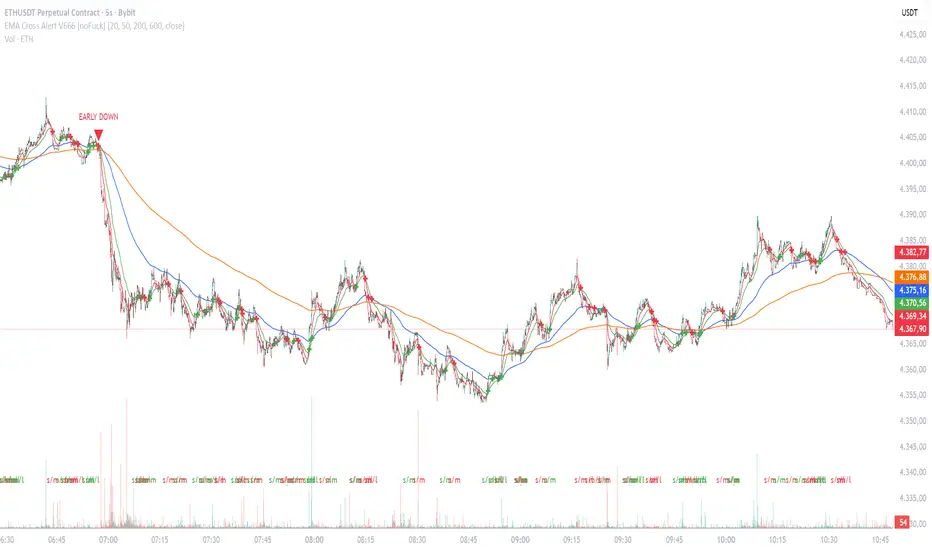
EMA Cross Alert V666 [noFuck]EMA Cross Alert — What it does
EMA Cross Alert watches three EMAs (Short, Mid, Long), detects their crossovers, and reports exactly one signal per bar by priority: EARLY > Short/Mid > Mid/Long > Short/Long. Optional EARLY mode pings when Short crosses Long while Mid is still between them—your polite early heads-up.
Why you might like it
Three crossover types: s/m, m/l, s/l
EARLY detection: earlier hints, not hype
One signal per bar: less noise, more focus
Clear visuals: tags, big cross at signal price, EARLY triangles
Alert-ready: dynamic alert text on bar close + static alertconditions for UI
Inputs (plain English)
Short/Mid/Long EMA length — how fast each EMA reacts
Extra EMA length (visual only) — context EMA; does not affect signals
Price source — e.g., Close
Show cross tags / EARLY triangles / large cross — visual toggles
Enable EARLY signals (Short/Long before Mid) — turn early pings on/off
Count Mid EMA as "between" even when equal (inclusive) — ON: Mid counts even if exactly equal to Short or Long; OFF (default): Mid must be strictly between them
Enable dynamic alerts (one per bar close) — master alert switch
Alert on Short/Mid, Mid/Long, Short/Long, EARLY — per-signal alert toggles
Quick tips
Start with defaults; if you want more EARLY on smooth/low-TF markets, turn “inclusive” ON
Bigger lengths = calmer trend-following; smaller = faster but choppier
Combine with volume/structure/risk rules—the indicator is the drummer, not the whole band
Disclaimer
Alerts, labels, and triangles are not trade ideas or financial advice. They are informational signals only. You are responsible for entries, exits, risk, and position sizing. Past performance is yesterday; the future is fashionably late.
Credits
Built with the enthusiastic help of Code Copilot (AI)—massively involved, shamelessly proud, and surprisingly good at breakfasting on exponential moving averages.
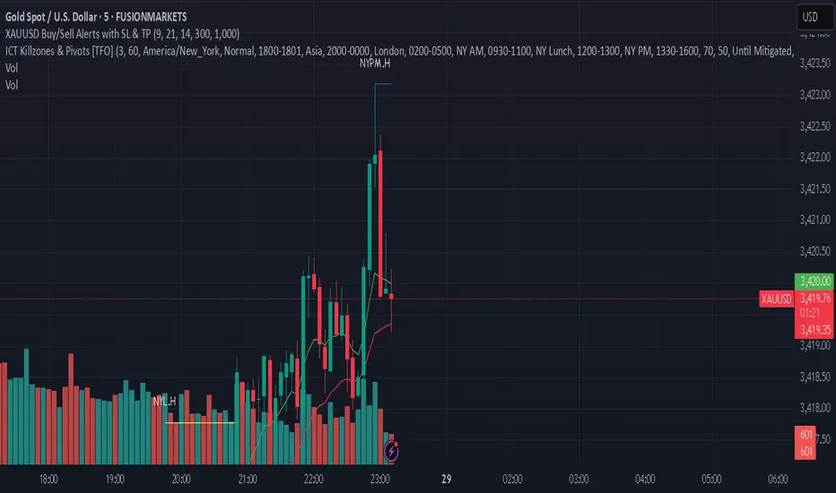
XAUUSD Buy/Sell Alerts with SL & TPThis custom TradingView indicator identifies high-probability buy and sell signals on XAUUSD using EMA crossovers combined with RSI confirmation. Designed for precision entries, it automatically calculates optimal Stop Loss (SL) and Take Profit (TP) levels based on user-defined pip distances.
Key Features:
Fast and Slow EMA crossover for trend direction
RSI filter for momentum confirmation
Dynamic SL and TP levels to manage risk and reward
Visual buy/sell signals plotted on chart
Real-time alerts with detailed messages including entry price, SL, and TP
Suitable for multiple timeframes and trading styles
Perfect for traders seeking clear signals with built-in risk management for scalping or swing trading XAUUSD.
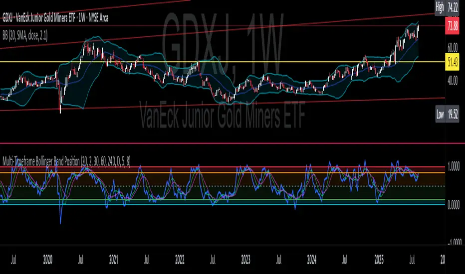
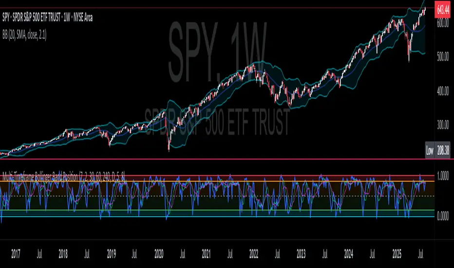
CNS - Multi-Timeframe Bollinger Band OscillatorMy hope is to optimize the settings for this indicator and reintroduce it as a "strategy" with suggested position entry and exit points shown in the price pane.
I’ve been having good results setting the “Bollinger Band MA Length” in the Input tab to between 5 and 10. You can use the standard 20 period, but your results will not be as granular.
This indicator has proven very good at finding local tops and bottoms by combining data from multiple timeframes. Use BB timeframes that are lower than the timeframe you are viewing in your price pane.
The default settings work best on the weekly timeframe, but can be adjusted for most timeframes including intraday.
Be cognizant that the indicator, like other oscillators, does occasionally produce divergences at tops and bottoms.
Any feedback is appreciated.
Overview
This indicator is an oscillator that measures the normalized position of the price relative to Bollinger Bands across multiple timeframes. It takes the price's position within the Bollinger Bands (calculated on different timeframes) and averages those positions to create a single value that oscillates between 0 and 1. This value is then plotted as the oscillator, with reference lines and colored regions to help interpret the price's relative strength or weakness.
How It Works
Bollinger Band Calculation:
The indicator uses a custom function f_getBBPosition() to calculate the position of the price within Bollinger Bands for a given timeframe.
Price Position Normalization:
For each timeframe, the function normalizes the price's position between the upper and lower Bollinger Bands.
It calculates three positions based on the high, low, and close prices of the requested timeframe:
pos_high = (High - Lower Band) / (Upper Band - Lower Band)
pos_low = (Low - Lower Band) / (Upper Band - Lower Band)
pos_close = (Close - Lower Band) / (Upper Band - Lower Band)
If the upper band is not greater than the lower band or if the data is invalid (e.g., na), it defaults to 0.5 (the midline).
The average of these three positions (avg_pos) represents the normalized position for that timeframe, ranging from 0 (at the lower band) to 1 (at the upper band).
Multi-Timeframe Averaging:
The indicator fetches Bollinger Band data from four customizable timeframes (default: 30min, 60min, 240min, daily) using request.security() with lookahead=barmerge.lookahead_on to get the latest available data.
It calculates the normalized position (pos1, pos2, pos3, pos4) for each timeframe using f_getBBPosition().
These four positions are then averaged to produce the final avg_position:avg_position = (pos1 + pos2 + pos3 + pos4) / 4
This average is the oscillator value, which is plotted and typically oscillates between 0 and 1.
Moving Averages:
Two optional moving averages (MA1 and MA2) of the avg_position can be enabled, calculated using simple moving averages (ta.sma) with customizable lengths (default: 5 and 10).
These can be potentially used for MA crossover strategies.
What Is Being Averaged?
The oscillator (avg_position) is the average of the normalized price positions within the Bollinger Bands across the four selected timeframes. Specifically:It averages the avg_pos values (pos1, pos2, pos3, pos4) calculated for each timeframe.
Each avg_pos is itself an average of the normalized positions of the high, low, and close prices relative to the Bollinger Bands for that timeframe.
This multi-timeframe averaging smooths out short-term fluctuations and provides a broader perspective on the price's position within the volatility bands.
Interpretation
0.0 The price is at or below the lower Bollinger Band across all timeframes (indicating potential oversold conditions).
0.15: A customizable level (green band) which can be used for exiting short positions or entering long positions.
0.5: The midline, where the price is at the average of the Bollinger Bands (neutral zone).
0.85: A customizable level (orange band) which can be used for exiting long positions or entering short positions.
1.0: The price is at or above the upper Bollinger Band across all timeframes (indicating potential overbought conditions).
The colored regions and moving averages (if enabled) help identify trends or crossovers for trading signals.
Example
If the 30min timeframe shows the close at the upper band (position = 1.0), the 60min at the midline (position = 0.5), the 240min at the lower band (position = 0.0), and the daily at the upper band (position = 1.0), the avg_position would be:(1.0 + 0.5 + 0.0 + 1.0) / 4 = 0.625
This value (0.625) would plot in the orange region (between 0.85 and 0.5), suggesting the price is relatively strong but not at an extreme.
Notes
The use of lookahead=barmerge.lookahead_on ensures the indicator uses the latest available data, making it more real-time, though its effectiveness depends on the chart timeframe and TradingView's data feed.
The indicator’s sensitivity can be adjusted by changing bb_length ("Bollinger Band MA Length" in the Input tab), bb_mult ("Bollinger Band Standard Deviation," also in the Input tab), or the selected timeframes.

Multi-Timeframe Bollinger BandsMy hope is to optimize the settings for this indicator and reintroduce it as a "strategy" with suggested position entry and exit points shown in the price pane.
I’ve been having good results setting the “Bollinger Band MA Length” in the Input tab to between 5 and 10. You can use the standard 20 period, but your results will not be as granular.
This indicator has proven very good at finding local tops and bottoms by combining data from multiple timeframes. Use timeframes that are lower than the timeframe you are viewing in your price pane. Be cognizant that the indicator, like other oscillators, does occasionally produce divergences at tops and bottoms.
Any feedback is appreciated.
Overview
This indicator is an oscillator that measures the normalized position of the price relative to Bollinger Bands across multiple timeframes. It takes the price's position within the Bollinger Bands (calculated on different timeframes) and averages those positions to create a single value that oscillates between 0 and 1. This value is then plotted as the oscillator, with reference lines and colored regions to help interpret the price's relative strength or weakness.
How It Works
Bollinger Band Calculation:
The indicator uses a custom function f_getBBPosition() to calculate the position of the price within Bollinger Bands for a given timeframe.
Price Position Normalization:
For each timeframe, the function normalizes the price's position between the upper and lower Bollinger Bands.
It calculates three positions based on the high, low, and close prices of the requested timeframe:
pos_high = (High - Lower Band) / (Upper Band - Lower Band)
pos_low = (Low - Lower Band) / (Upper Band - Lower Band)
pos_close = (Close - Lower Band) / (Upper Band - Lower Band)
If the upper band is not greater than the lower band or if the data is invalid (e.g., na), it defaults to 0.5 (the midline).
The average of these three positions (avg_pos) represents the normalized position for that timeframe, ranging from 0 (at the lower band) to 1 (at the upper band).
Multi-Timeframe Averaging:
The indicator fetches Bollinger Band data from four customizable timeframes (default: 30min, 60min, 240min, daily) using request.security() with lookahead=barmerge.lookahead_on to get the latest available data.
It calculates the normalized position (pos1, pos2, pos3, pos4) for each timeframe using f_getBBPosition().
These four positions are then averaged to produce the final avg_position:avg_position = (pos1 + pos2 + pos3 + pos4) / 4
This average is the oscillator value, which is plotted and typically oscillates between 0 and 1.
Moving Averages:
Two optional moving averages (MA1 and MA2) of the avg_position can be enabled, calculated using simple moving averages (ta.sma) with customizable lengths (default: 5 and 10).
These can be potentially used for MA crossover strategies.
What Is Being Averaged?
The oscillator (avg_position) is the average of the normalized price positions within the Bollinger Bands across the four selected timeframes. Specifically:It averages the avg_pos values (pos1, pos2, pos3, pos4) calculated for each timeframe.
Each avg_pos is itself an average of the normalized positions of the high, low, and close prices relative to the Bollinger Bands for that timeframe.
This multi-timeframe averaging smooths out short-term fluctuations and provides a broader perspective on the price's position within the volatility bands.
Interpretation
0.0 The price is at or below the lower Bollinger Band across all timeframes (indicating potential oversold conditions).
0.15: A customizable level (green band) which can be used for exiting short positions or entering long positions.
0.5: The midline, where the price is at the average of the Bollinger Bands (neutral zone).
0.85: A customizable level (orange band) which can be used for exiting long positions or entering short positions.
1.0: The price is at or above the upper Bollinger Band across all timeframes (indicating potential overbought conditions).
The colored regions and moving averages (if enabled) help identify trends or crossovers for trading signals.
Example
If the 30min timeframe shows the close at the upper band (position = 1.0), the 60min at the midline (position = 0.5), the 240min at the lower band (position = 0.0), and the daily at the upper band (position = 1.0), the avg_position would be:(1.0 + 0.5 + 0.0 + 1.0) / 4 = 0.625
This value (0.625) would plot in the orange region (between 0.85 and 0.5), suggesting the price is relatively strong but not at an extreme.
Notes
The use of lookahead=barmerge.lookahead_on ensures the indicator uses the latest available data, making it more real-time, though its effectiveness depends on the chart timeframe and TradingView's data feed.
The indicator’s sensitivity can be adjusted by changing bb_length ("Bollinger Band MA Length" in the Input tab), bb_mult ("Bollinger Band Standard Deviation," also in the Input tab), or the selected timeframes.
Multi-Timeframe Bollinger Band PositionBeta version.
My hope is to optimize the settings for this indicator and reintroduce it as a "strategy" with suggested position entry and exit points shown in the price pane.
Any feedback is appreciated.
Overview
This indicator is an oscillator that measures the normalized position of the price relative to Bollinger Bands across multiple timeframes. It takes the price's position within the Bollinger Bands (calculated on different timeframes) and averages those positions to create a single value that oscillates between 0 and 1. This value is then plotted as the oscillator, with reference lines and colored regions to help interpret the price's relative strength or weakness.
How It Works
Bollinger Band Calculation:
The indicator uses a custom function f_getBBPosition() to calculate the position of the price within Bollinger Bands for a given timeframe.
Price Position Normalization:
For each timeframe, the function normalizes the price's position between the upper and lower Bollinger Bands.
It calculates three positions based on the high, low, and close prices of the requested timeframe:
pos_high = (High - Lower Band) / (Upper Band - Lower Band)
pos_low = (Low - Lower Band) / (Upper Band - Lower Band)
pos_close = (Close - Lower Band) / (Upper Band - Lower Band)
If the upper band is not greater than the lower band or if the data is invalid (e.g., na), it defaults to 0.5 (the midline).
The average of these three positions (avg_pos) represents the normalized position for that timeframe, ranging from 0 (at the lower band) to 1 (at the upper band).
Multi-Timeframe Averaging:
The indicator fetches Bollinger Band data from four customizable timeframes (default: 30min, 60min, 240min, daily) using request.security() with lookahead=barmerge.lookahead_on to get the latest available data.
It calculates the normalized position (pos1, pos2, pos3, pos4) for each timeframe using f_getBBPosition().
These four positions are then averaged to produce the final avg_position:avg_position = (pos1 + pos2 + pos3 + pos4) / 4
This average is the oscillator value, which is plotted and typically oscillates between 0 and 1.
Moving Averages:
Two optional moving averages (MA1 and MA2) of the avg_position can be enabled, calculated using simple moving averages (ta.sma) with customizable lengths (default: 5 and 10).
These can be potentially used for MA crossover strategies.
What Is Being Averaged?
The oscillator (avg_position) is the average of the normalized price positions within the Bollinger Bands across the four selected timeframes. Specifically:It averages the avg_pos values (pos1, pos2, pos3, pos4) calculated for each timeframe.
Each avg_pos is itself an average of the normalized positions of the high, low, and close prices relative to the Bollinger Bands for that timeframe.
This multi-timeframe averaging smooths out short-term fluctuations and provides a broader perspective on the price's position within the volatility bands.
Interpretation:
0.0 The price is at or below the lower Bollinger Band across all timeframes (indicating potential oversold conditions).
0.15: A customizable level (green band) which can be used for exiting short positions or entering long positions.
0.5: The midline, where the price is at the average of the Bollinger Bands (neutral zone).
0.85: A customizable level (orange band) which can be used for exiting long positions or entering short positions.
1.0: The price is at or above the upper Bollinger Band across all timeframes (indicating potential overbought conditions).
The colored regions and moving averages (if enabled) help identify trends or crossovers for trading signals.
Example:
If the 30min timeframe shows the close at the upper band (position = 1.0), the 60min at the midline (position = 0.5), the 240min at the lower band (position = 0.0), and the daily at the upper band (position = 1.0), the avg_position would be:(1.0 + 0.5 + 0.0 + 1.0) / 4 = 0.625
This value (0.625) would plot in the orange region (between 0.85 and 0.5), suggesting the price is relatively strong but not at an extreme.
Notes:
The use of lookahead=barmerge.lookahead_on ensures the indicator uses the latest available data, making it more real-time, though its effectiveness depends on the chart timeframe and TradingView's data feed.
The indicator’s sensitivity can be adjusted by changing bb_length ("Bollinger Band MA Length" in the Input tab), bb_mult ("Bollinger Band Standard Deviation," also in the Input tab), or the selected timeframes.
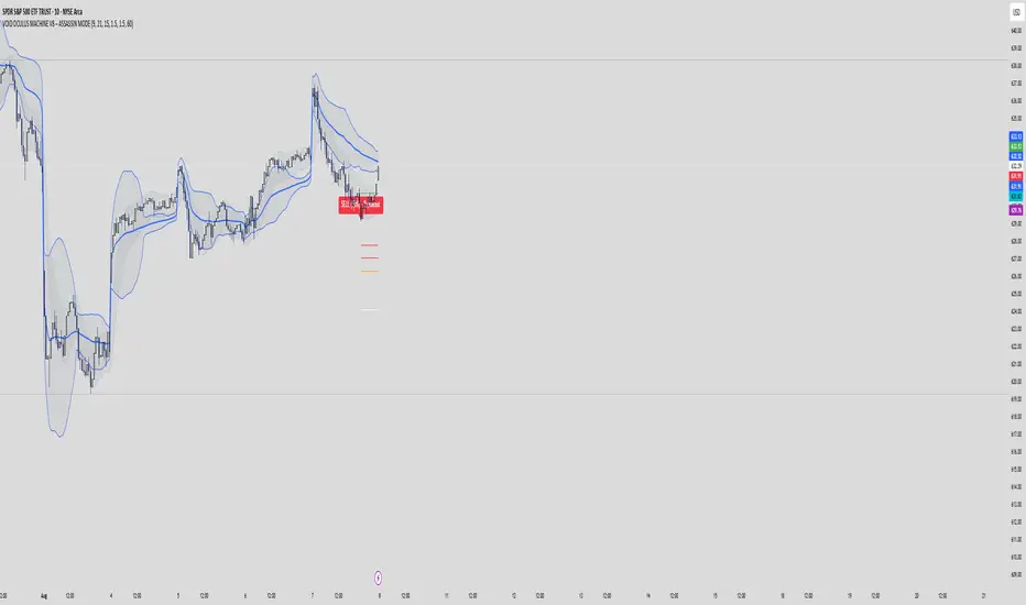
VOID OCULUS MACHINE V8 – ASSASSIN MODEVOID OCULUS MACHINE V8 – ASSASSIN MODE
Version 8.0 | Pine Script v6
Purpose & Originality
VOID OCULUS MACHINE V8 – ASSASSIN MODE brings together four advanced trading filters—EMA crossovers, TRIX momentum, VWAP band positioning, and a proprietary “Predictive Cloud”—into a single, high-precision entry system. Rather than relying on any one signal, it calculates a confidence score combining trend, momentum, volume, and volatility cues, then triggers only the highest-probability setups once a user-defined threshold is met. This multi-layer architecture offers traders laser-focused entries (“Assassin Mode”) with built-in risk (stop) and reward (targets) visualization.
How It Works & Component Rationale
EMA Trend Alignment
Fast EMA (9) vs. Slow EMA (21): Captures short-term versus medium-term trend. A bullish bias requires EMA9 > EMA21, bearish bias EMA9 < EMA21.
TRIX Momentum Filter
A triple-smoothed EMA oscillator over 15 bars, expressed as a percentage change. Positive TRIX confirms upward momentum; negative TRIX confirms downward momentum.
Gaussian Noise Reduction
Dual 5-period EMA smoothing of price removes short-term noise, creating a “cloud base.” Entries only fire when price interacts favorably with this smoothed baseline.
VWAP Band Confirmation (Optional)
Calculates session VWAP ± one standard deviation over 20 bars, plotting upper/lower bands. Traders can require price to sit above/below VWAP mid for trend confirmation.
Predictive Cloud Overlay
A dynamic band (Gaussian ± ATR) forecasts a near-term “value zone.” Pullback and reversal entries can occur as price re-enters or breaks out of this cloud.
Confidence Scoring
Starts at 0 and adds:
+30 for EMA trend alignment (bull or bear)
+20 for volume spike (>20-bar SMA)
+20 for non-zero TRIX slope
+20 for ATR expansion (volatility ramping)
+10 if price is above or below VWAP mid (if VWAP filter is enabled)
Only fires signals when confidence ≥ 60% (configurable), ensuring multi-factor confluence.
Entry Type Differentiation
Breakout: Price pierces prior 10-bar high/low on volume and ATR expansion.
Pullback: Trend bias plus a crossover of price with EMA9.
Reversal: Price crosses back into the Predictive Cloud from outside, confirmed by VWAP cross.
Automated Trade Visualization
On each signal, clears previous objects, plots a “BUY (xx%) – ” or “SELL (xx%) – ” label, four tiered ATR-based targets (1×, 1.5×, 2×, 3.5×), and a stop-loss (ATR × 1.5).
Inputs & Customization
Input Description Default
Fast EMA Length for short-term trend EMA 9
Slow EMA Length for medium-term trend EMA 21
TRIX Length Period for triple-smoothed momentum oscillator 15
Stop Multiplier ATR multiple for stop-loss distance 1.5
Target Multiplier ATR multiple for first profit target 1.5
Enable VWAP Filter Require price alignment above/below VWAP mid On
Minimum Confidence Confidence % threshold to trigger a signal 60
Show Predictive Cloud Toggle the Gaussian ± ATR cloud on/off On
How to Use
Apply to Chart: Suitable on 5 m–1 h timeframes for swing entries.
Adjust Confidence & Filters: Raise the Minimum Confidence to tighten setups; disable VWAP filter for pure price/momentum plays.
Read Signals:
“BUY (75%) – Breakout” label means 75% confluence across filters, triggered by a breakout entry type.
Four colored horizontal lines mark TP1–TP4; a red line marks your stop.
Manage the Trade:
Use the plotted stop-loss line; scale out at targets or trail behind the Predictive Cloud.
Unique Value
VOID OCULUS MACHINE V8 stands out by quantifying multi-dimensional market context into a single confidence score and providing automated trade object plotting—no more manual target calculations or cluttered charts. Its “Assassin Mode” ensures only the most compelling setups trigger, saving traders time and reducing noise.
Disclaimer
This indicator is for educational purposes. Past performance does not guarantee future results. Always backtest across symbols/timeframes, combine with personal discretion, and apply strict risk management before trading live.
Cumulative Volume Delta (SB-1) 2.0
📈 Cumulative Volume Delta (CVD) — Stair-Step + Threshold Alerts
🔍 Overview
This Cumulative Volume Delta (CVD) tool visualizes aggressive buying and selling pressure in the market by plotting candlestick-style bars based on volume delta. It helps traders understand which side — buyers or sellers — is exerting more control on lower timeframes and highlights momentum shifts through stair-step patterns and delta threshold breaks. Resets to zero at EOD
Ideal for futures traders, scalpers, and intraday strategists looking for orderflow-based confirmation.
🧠 What Is CVD?
CVD (Cumulative Volume Delta) measures the difference between market buys and sells over a specific timeframe. When the delta is rising, it suggests buyers are being more aggressive. Falling delta suggests seller dominance.
This script aggregates volume delta from a lower timeframe and plots it in a higher timeframe context, allowing you to track microstructure shifts within larger candles.
📊 Features
✅ CVD Candlesticks
Each bar represents volume delta as an OHLC-style candle using:
Open: Delta at the start of the bar
High/Low: Peak delta range
Close: Final delta value at bar close
Teal candles = Net buying pressure
Red candles = Net selling pressure
✅ Threshold Levels (Key Visual Zones)
The script includes horizontal dashed lines at:
+5,000 and +10,000 → Signify strong buying pressure
-5,000 and -10,000 → Signify strong selling pressure
0 line → Neutrality line (no net pressure)
These levels act as volume-based support/resistance zones and breakout confirmation tools. For example:
A CVD cross above +5,000 shows buyers taking control
A CVD cross above +10,000 implies strong bullish momentum
A CVD cross below -5,000 or -10,000 signals intense selling pressure
📈 Stair-Step Pattern Detection
Detects two specific volume-based continuation setups:
Bullish Stair-Step: Both the high and low of the CVD candle are higher than the previous candle
Bearish Stair-Step: Both the high and low of the CVD candle are lower than the previous candle
These patterns often appear during trending moves and serve as confirmation of strength or continuation.
Visual markers:
🟢 Green triangles below bars = Bullish stair-step
🔴 Red triangles above bars = Bearish stair-step
🔔 Alert Conditions
Get real-time alerts when:
Bullish Stair-Step is detected
Bearish Stair-Step is detected
CVD crosses above +5,000
CVD crosses below -5,000
📢 Alerts only trigger on crossover, not every time CVD remains above or below. This avoids repetitive notifications.
⚙️ Inputs & Customization
Anchor Timeframe: The higher timeframe to which CVD data is applied (default: 1D)
Lower Timeframe: The timeframe used to calculate the CVD delta (default: 5 minutes)
Optional Override: Use custom timeframe toggle to force your own micro timeframe
📌 How to Use This CVD Indicator (Step-by-Step Guide)
✅ 1. Confirm Bias Using the Zero Line
The zero line (0 CVD) represents neutral pressure — neither buyers nor sellers are dominating.
Use it as your first filter:
🔼 If CVD is above 0 and rising → Buyer control
🔽 If CVD is below 0 and falling → Seller control
🧠 Tip: CVD rising while price is consolidating may signal hidden buyer interest.
✅ 2. Watch for Crosses of Key Levels: +5,000 and +10,000
These levels act as momentum thresholds:
Level Signal Type What It Means
+5,000 Buyer breakout Buyers are starting to dominate
+10,000 Strong bull bias Strong institutional or algorithmic buying flow
-5,000 Seller breakout Sellers are taking control
-10,000 Strong bear bias Heavy selling pressure is entering the market
Wait for CVD to cross above +5K or below -5K to confirm the active side.
Use these crossovers as entry triggers, breakout confirmations, or trade filters.
🔔 Alerts fire only when the level is first crossed, not every bar above/below.
✅ 3. Use Stair-Step Patterns for Continuation Confirmation
The indicator shows stair-step patterns using triangle signals:
🟢 Green triangle below bar = Bullish stair-step
Suggests a higher high and higher low in delta → buyers stepping up
🔴 Red triangle above bar = Bearish stair-step
Suggests lower highs and lower lows in delta → selling pressure building
Use stair-step signals:
To confirm a continuation of trend
As an entry or add-on signal
Especially after a threshold breakout
🧠 Example: If CVD breaks above +5K and forms bullish stairs → confirms strong trend, ideal for momentum entries.
✅ 4. Combine with Price Action or Structure
CVD works best when used with price, not in isolation. For example:
📉 Price makes a new low but CVD doesn’t → potential bullish divergence
📈 CVD surges while price lags → buyers are absorbing, breakout likely
Use it with:
VWAP
Orderblocks
Liquidity sweeps
Break of market structure/MSS/BOS
✅ 5.
Set Anchor Timeframe = Daily
Set Lower Timeframe = 5 minutes (default)
This lets you:
See intraday flow inside daily bars
Confirm whether a daily candle is being built on net buying or selling
🧠 You’re essentially seeing intra-bar aggression within a bigger time structure.
🧭 Example Trading Setup
Bullish Scenario:
CVD is rising and above 0
CVD crosses above +5,000 → alert fires
Green stair-step appears
Price breaks local resistance or liquidity sweep completes
✅ Consider long entry with structure and CVD alignment
🎯 Place stops below last stair-step or structural low
📌 Final Notes
This tool does not repaint and is designed to work in real-time across all futures, crypto, and equity instruments that support volume data. If your symbol does not provide volume, the script will notify you.
Use it in confluence with VWAP, liquidity zones, or structure breaks for high-confidence trades.

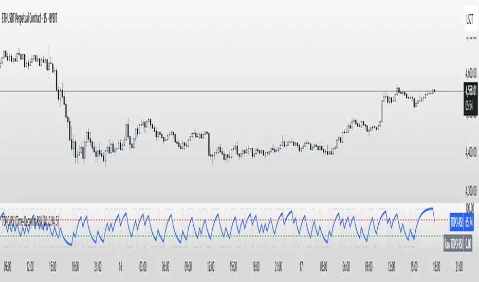
TDPO-RSI (Time-Decaying Percentile RSI)TDPO-RSI (Time-Decaying Percentile RSI)
TDPO-RSI is a modern, statistically-enhanced momentum indicator that improves on traditional RSI by using percentile-based analysis with exponential time decay. Instead of averaging gains and losses equally, this indicator ranks them by size and weights recent data more heavily—resulting in a more responsive and noise-resistant signal.
How it works:
Calculates percentile rank of gains and losses over a lookback window
Applies a decay factor (lambda) to give more weight to recent price action
Outputs a percentile-based RSI value between 0 and 100
Optional smoothing via EMA for clearer crossover signals
Key Uses:
Identify overbought/oversold zones (default: 70/30)
Use raw vs. smoothed RSI crossovers for entries
Detect momentum shifts earlier than traditional RSI
Suitable for scalping, trend continuation, and reversal setups
Inputs:
Lookback Length: Number of bars used for percentile calculation
Decay Factor (lambda): How quickly older data fades in influence (0.80–0.99)
Smoothing EMA: Smooths the final output to reduce noise
Tip: Combine with price structure and volume for best results. Higher timeframes can be used for trend context, while lower timeframes help with precise entries.
This tool is ideal for traders who want adaptive momentum analysis rooted in statistical behavior.
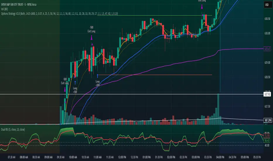
Options Strategy V2.0📈 Options Strategy V2.0 – Intraday Reversal-Resilient Momentum System
Overview:
This strategy is designed specifically for intraday SPY, TSLA, MSFT, etc. options trading (0DTE or 1DTE), using high-probability signals derived from a confluence of technical indicators: EMA crossovers, RSI thresholds, ATR-based risk control, and volume spikes. The strategy aims to capture strong directional moves while avoiding overtrading, thanks to a built-in cooldown logic and optional time/session filters.
⚙️ Core Concept
The strategy executes trades only in the direction of the prevailing trend, determined by short- and long-term Exponential Moving Averages (EMA). Entry signals are generated when the Relative Strength Index (RSI) confirms momentum in the direction of the trend, and volume spikes suggest institutional activity.
To increase adaptability and user control, it includes a highly customizable parameter set for both long and short entries independently.
📌 Key Features
✅ Trend-Following Logic
Long entries are only allowed when EMA(short) > EMA(long)
Short entries are only allowed when EMA(short) < EMA(long)
✅ RSI Confirmation
Long: Requires RSI crossover above a configurable threshold
Short: Requires RSI crossunder below a configurable threshold
Optional rejection filters: Entry blocked above/below specific RSI extremes
✅ Volume Spike Filter
Confirms institutional participation by comparing current volume to an average multiplied by a user-defined factor.
✅ ATR-Based Risk Management
Both Stop Loss (SL) and Take Profit (TP) are dynamically calculated using ATR × a multiplier.
TP/SL ratio is fully configurable.
✅ Cooldown Control
After every trade, the system waits for a set number of bars before allowing new entries.
This prevents overtrading and increases signal quality.
Optionally, cooldown is ignored for reversal trades, ensuring the system can react immediately to a confirmed trend change.
✅ Candle Body Filter (Noise Control)
Avoids trades on candles with too small bodies relative to wicks (often noise or indecision candles).
✅ VWAP Confirmation (Optional)
Ensures price is trading above VWAP for long entries, or below for short entries.
✅ Time & Session Filters
Trades only during regular market hours (09:30–16:00 EST).
No-trade zone (e.g., 14:15–15:45 EST) to avoid low-liquidity traps or late-day whipsaws.
✅ End-of-Day Auto Close
All open positions are force-closed at 15:55 EST, protecting against overnight risk (especially relevant for 0DTE options).
📊 Visual Aids
EMA plots show trend direction
VWAP line provides real-time mean-reversion context
Stop Loss and Take Profit lines appear dynamically with each trade
Alerts notify of entry signals and exit triggers
🔧 Customization Panel
Nearly every element of the strategy can be tailored:
EMA lengths (short and long, for both sides)
RSI thresholds and length
ATR length, SL multiplier, and TP/SL ratio
Volume spike sensitivity
Minimum EMA distance filter
Candle body ratio filter
Session restrictions
Cooldown logic (duration + reversal exception)
This makes the strategy extremely versatile, allowing both conservative and aggressive configurations depending on the trader’s profile and the market context.
📌 Example Use Case: SPY Options (0DTE or 1DTE)
This system was designed and tested specifically for SPY and other intraday options trading, where:
Delta is around 0.50 or higher
Trades are short-lived (often 1–5 candles)
You aim to trade 1–3 signals per day, filtering out weak entries
🚫 Important Notes
It is not a scalping strategy; it relies on confirmed breakouts with trend support
No pyramiding or re-entries without cooldown to preserve risk integrity
Should be used with real-time alerts and manual broker execution
📈 Alerts Included
📈 Long Entry Signal
📉 Short Entry Signal
⚠️ Auto-closed all positions at 15:55 EST
✅ Proven Settings – Real Trades + Backtest Results
The current version of the strategy includes the optimal settings I’ve arrived at through extensive backtesting, as well as 3 months of real trading with consistent profitability. These results reflect real-world execution under live market conditions using 0DTE SPY options, with disciplined trade management and risk control.
🧠 Final Thoughts
Options Strategy V2.0 is a robust, highly tunable intraday strategy that blends momentum, trend-following, and volume confirmation. It is ideal for disciplined traders focused on SPY or other 0DTE/1DTE options, and it includes guardrails to reduce false signals and improve execution timing.
Perfect for those who seek precision, flexibility, and risk-defined setups—not blind automation.
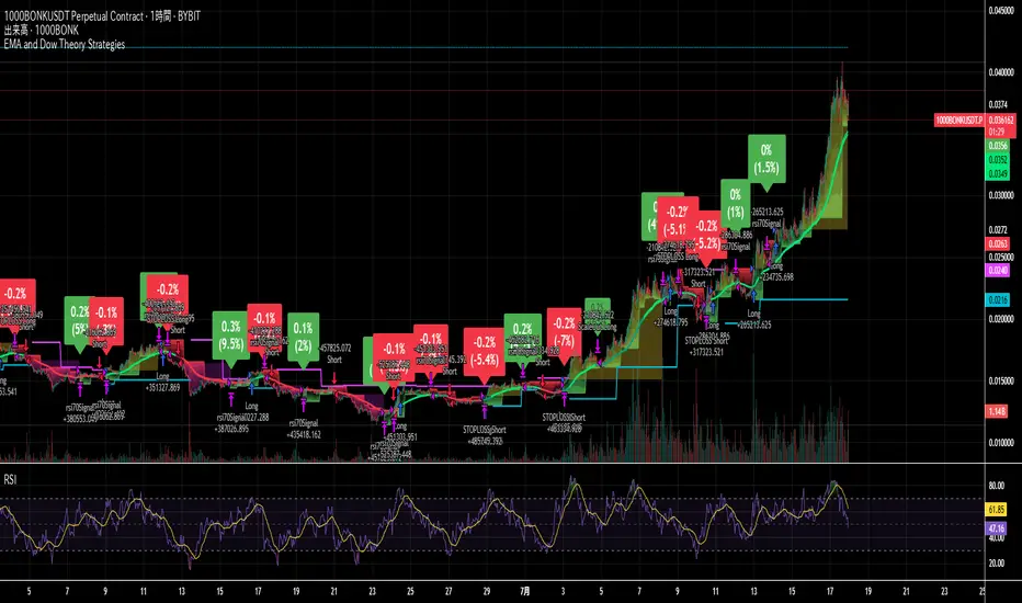
EMA and Dow Theory Strategies🌐 Strategy Description
📘 Overview
This is a hybrid strategy that combines EMA crossovers, Dow Theory swing logic, and multi-timeframe trend overlays. It is suitable for intraday to short-term trading on any asset class: crypto, forex, stocks, and indices.
The strategy provides precise entry/exit signals, dynamic stop-loss and scale-out, and highly visual trade guidance.
🧠 Key Features
・Dual EMA crossover system (applied to both symbol and external index)
・Dow Theory-based swing high/low detection for trend confirmation
・Visual overlay of higher timeframe swing trend (htfTrend)
・RSI filter to avoid overbought/oversold entries
・Dynamic partial take-profit when trend weakens
・Custom stop-loss (%) control
・Visualized trade PnL labels directly on chart
・Alerts for entry, stop-loss, partial exit
・Gradient background zones for swing zones and trend visualization
・Auto-tracked metrics: APR, drawdown, win rate, equity curve
⚙️ Input Parameters
| Parameter | Description |
| ------------------------- | -------------------------------------------------------- |
| Fast EMA / Slow EMA | Periods for detecting local trend via EMAs |
| Index Fast EMA / Slow EMA | EMAs applied to external reference index |
| StopLoss | Maximum loss threshold in % |
| ScaleOut Threshold | Scale-out percentage when trend changes color |
| RSI Period / Levels | RSI period and overbought/oversold levels |
| Swing Detection Length | Number of bars used to detect swing highs/lows |
| Stats Display Options | Toggle PnL labels and position of statistics table |
🧭 About htfTrend (Higher Timeframe Trend)
The script includes a higher timeframe trend (htfTrend) calculated using Dow Theory (pivot highs/lows).
This trend is only used for visual guidance, not for actual entry conditions.
Why? Strictly filtering trades by higher timeframe often leads to missed opportunities and low frequency.
By keeping htfTrend visual-only, traders can still refer to macro structure but retain trade flexibility.
Use it as a contextual tool, not a constraint.
ストラテジー説明
📘 概要
本ストラテジーは、EMAクロスオーバー、ダウ理論によるスイング判定、**上位足トレンドの視覚表示(htfTrend)**を組み合わせた複合型の短期トレーディング戦略です。
仮想通貨・FX・株式・指数など幅広いアセットに対応し、デイトレード〜スキャルピング用途に適しています。
動的な利確/損切り、視覚的にわかりやすいエントリー/イグジット、統計表示を搭載しています。
🧠 主な機能
・対象銘柄+外部インデックスのEMAクロスによるトレンド判定
・ダウ理論に基づいたスイング高値・安値検出とトレンド判断
・上位足スイングトレンド(htfTrend)の視覚表示
・RSIフィルターによる過熱・売られすぎの回避
・トレンドの弱まりに応じた部分利確(スケールアウト)
・**損切り閾値(%)**をカスタマイズ可能
・チャート上に損益ラベル表示
・アラート完備(エントリー・決済・部分利確)
・トレンドゾーンを可視化する背景グラデーション
・勝率・ドローダウン・APR・資産増加率などの自動表示
| 設定項目名 | 説明内容 |
| --------------------- | -------------------------- |
| Fast EMA / Slow EMA | 銘柄に対して使用するEMAの期間設定 |
| Index Fast / Slow EMA | 外部インデックスのEMA設定 |
| 損切り(StopLoss) | 損切りラインのしきい値(%で指定) |
| 部分利確しきい値 | トレンド弱化時にスケールアウトする割合(%) |
| RSI期間・水準 | RSI計算期間と、過熱・売られすぎレベル設定 |
| スイング検出期間 | スイング高値・安値の検出に使用するバー数 |
| 統計表示の切り替え | 損益ラベルや統計テーブルの表示/非表示選択 |
🧭 上位足トレンド(htfTrend)について
本スクリプトには、上位足でのスイング高値・安値の更新に基づく**htfTrend(トレンド判定)が含まれています。
これは視覚的な参考情報であり、エントリーやイグジットには直接使用されていません。**
その理由は、上位足を厳密にロジックに組み込むと、トレード機会の損失が増えるためです。
このスクリプトでは、**判断の補助材料として「表示のみに留める」**設計を採用しています。
→ 裁量で「利確を早める」「逆張りを避ける」判断に活用可能です。
AZ Dynamic Trend Indicator with Heikin-Ashi### Dynamic Trend Indicator with Heikin-Ashi (v2.7)
**Effortlessly identify trends and reversals** with this versatile tool combining multi-timeframe analysis, adaptive moving averages, and Heikin-Ashi smoothing. Here's what it offers:
#### 🔍 **Core Features**
1. **Dual Timeframe Analysis**:
- Track trends on higher timeframes (e.g., 1H/D) while viewing signals on your current chart.
- Toggle between **Heikin-Ashi** or standard candles for cleaner trend visualization.
2. **8 Customizable MAs**:
- Choose from **ALMA, HMA, SMA, SWMA, VWMA, WMA, ZLEMA, or EMA** with adjustable periods.
- Unique "Trend Strength" metric: `(MA_Close - MA_Open) / (MA_High - MA_Low)` highlights momentum direction.
3. **Smart Signals**:
- **Entry/Exit**: Triangles mark crossovers between MA Close/Open.
- **Reversal Alerts**: Detects counter-trend moves within a user-defined window (default: 3 bars) after signals.
- Color-coded plots: Bullish (🟢), Bearish (🔴), Reversal Bull (🔵), Reversal Bear (🟠).
#### 🎨 **Visual Customization**
- Toggle **High/Low MA lines**, **Close line**, and **fill colors**.
- Adjust colors for all elements to match your chart theme.
- Hide signals or reversal markers as needed.
#### ⚙️ **Practical Use**
- **Trend Following**: Use the MA Close/Open crossover with trend fill colors to confirm direction.
- **Reversal Trading**: Capitalize on pullbacks with reversal signals (e.g., after a bearish signal, watch for Bull Reversal markers).
- **Multi-Timeframe Confirmation**: Avoid false signals by aligning higher-timeframe trends with your entries.
*Ideal for swing traders and trend riders!*
**Note**: Adjust `MA Period`, `Reversal Window`, and `Trend Timeframe` for your strategy. Disable Heikin-Ashi in choppy markets for faster reactions.
---
*Code v2.7 updates: Optimized reversal logic, added ALMA/ZLEMA support, and enhanced visual controls.*

Market Shift Levels [ChartPrime]Market Shift Levels
This indicator detects trend shifts and visualizes key market structure turning points using Hull Moving Average logic. It highlights potential areas of support and resistance where price is likely to react, empowering traders to spot early trend transitions.
Market Shift Levels are horizontal zones that mark the moment of a directional change in market behavior. These shifts are based on crossovers between two smoothed Hull Moving Averages (HMA), allowing the indicator to detect potential reversals with minimal lag.
Once a shift is detected:
A dashed horizontal Market Shift Level is plotted at the low (for bullish shift) or high (for bearish shift) of the candle.
These levels often become key reaction points during pullbacks and trend retests.
Volume or price labels are added when price wicks into these levels, helping traders gauge the strength of rejection or acceptance.
⯁ KEY FEATURES
Uses HMA-based logic to detect when price momentum shifts.
Plots clean Market Shift Levels (MSLs) that act as dynamic support and resistance.
Automatically colors bars and candles based on the price positioning relative to levels.
Labels wick-based retests with either:
Volume data of the 3-bar cluster (default).
Price level if toggled.
⯁ HOW TO USE
Look for trend shifts where the HMA crossover triggers a new level — this marks a possible structural pivot .
Use the horizontal level as a dynamic support or resistance zone — especially when price returns with wick rejections.
Watch for volume labels near the level — higher values signal stronger rejection and potential continuation.
Combine with confluence tools like Smart Money concepts or Fibonacci levels for added edge.
⯁ EXAMPLE SETUPS
After a bullish shift, wait for price to return and wick into the level — if volume spikes and candle closes strong, it’s a retest confirmation entry .
After a bearish shift, bearish wick rejections with volume may signal short re-entry zones .
⯁ CONCLUSION
The Market Shift Levels indicator offers a visual and data-backed approach to spotting trend reversals and critical retest zones. It’s a simple yet powerful tool to structure your trades around objective, repeatable market behavior — all in real-time.

CVD Strength | VTS Pro🔷 CVD Strength | VTS Pro
By Alireza Mossaheb
Description:
CVD Strength is a powerful tool designed to analyze market momentum by visualizing the Cumulative Volume Delta (CVD) using advanced techniques. This indicator provides a multi-timeframe view of volume delta behavior and highlights strong and weak bullish/bearish conditions based on volume spikes, candle size, and optional moving average filters.
Key Features:
Multi-timeframe CVD candle plotting with color-coded strength signals
Optional EMA (21), WMA (30), and SMA (50) overlays for trend filtering
Smart strength detection logic using volume, candle size, and moving average crossovers
Bullish and bearish crossover signals marked on chart
Customizable anchor and lower timeframes for flexible analysis
Alerts users when data vendor does not supply volume information
This script is particularly useful for identifying institutional buying/selling pressure and can be used effectively in both trend-following and mean-reversion strategies.

Trend Flow Trail [AlgoAlpha]OVERVIEW
This script overlays a custom hybrid indicator called the Money Flow Trail which combines a volatility-based trend-following trail with a volume-weighted momentum oscillator. It’s built around two core components: the AlphaTrail—a dynamic band system influenced by Hull MA and volatility—and a smoothed Money Flow Index (MFI) that provides insights into buying or selling pressure. Together, these tools are used to color bars, generate potential reversal markers, and assist traders in identifying trend continuation or exhaustion phases in any market or timeframe.
CONCEPTS
The AlphaTrail calculates a volatility-adjusted channel around price using the Hull Moving Average as the base and an EMA of range as the spread. It adaptively shifts based on price interaction to capture trend reversals while avoiding whipsaws. The direction (bullish or bearish) determines both the band being tracked and how the trail locks in. The Money Flow Index (MFI) is derived from hlc3 and volume, measuring buying vs selling pressure, and is further smoothed with a short Hull MA to reduce noise while preserving structure. These two systems work in tandem: AlphaTrail governs directional context, while MFI refines the timing.
FEATURES
Dynamic AlphaTrail line with regime switching logic that controls directional bias and bar coloring.
Smoothed MFI with gradient coloring to visually communicate pressure and exhaustion levels.
Overbought/oversold thresholds (80/20), mid-level (50), and custom extreme zones (90/10) for deeper signal granularity.
Built-in take-profit signal logic: crossover of MFI into overbought with bullish AlphaTrail, or into oversold with bearish AlphaTrail.
Visual fills between price and AlphaTrail for clearer confirmation during trend phases.
Alerts for regime shifts, MFI crossovers, trail interactions, and bar color regime changes.
USAGE
Add the indicator to any chart. Use the AlphaTrail plot to define trend context: bullish (trailing below price) or bearish (trailing above). MFI values give supporting confirmation—favor long setups when MFI is rising and above 50 in a bullish regime, and shorts when MFI is falling and below 50 in a bearish regime. The colored fills help visually track strength; sharp changes in MFI crossing 80/20 or 90/10 zones often precede pullbacks or reversals. Use the plotted circles as optional take-profit signals when MFI and trend are extended. Adjust AlphaTrail length/multiplier and MFI smoothing to better match the asset’s volatility profile.

Adaptive MACD Deluxe [AlgoAlpha]OVERVIEW
This script is an advanced rework of the classic MACD indicator, designed to be more adaptive, visually informative, and customizable. It enhances the original MACD formula using a dynamic feedback loop and a correlation-based weighting system that adjusts in real-time based on how deterministic recent price action is. The signal line is flexible, offering several smoothing types including Heiken Ashi, while the histogram is color-coded with gradients to help users visually identify momentum shifts. It also includes optional normalization by volatility, allowing MACD values to be interpreted as relative percentage moves, making the indicator more consistent across different assets and timeframes.
CONCEPTS
This version of MACD introduces a deterministic weight based on R-squared correlation with time, which modulates how fast or slow the MACD adapts to price changes. Higher correlation means smoother, slower MACD responses, and low correlation leads to quicker reaction. The momentum calculation blends traditional EMA math with feedback and damping components to create a smoother, less noisy series. Heiken Ashi is optionally used for signal smoothing to better visualize short-term trend bias. When normalization is enabled, the MACD is scaled by an EMA of the high-low range, converting it into a bounded, volatility-relative indicator. This makes extreme readings more meaningful across markets.
FEATURES
The script offers six distinct options for signal line smoothing: EMA, SMA, SMMA (RMA), WMA, VWMA, and a custom Heiken Ashi mode based on the MACD series. Each option provides a different response speed and smoothing behavior, allowing traders to match the indicator’s behavior to their strategy—whether it's faster reaction or reduced noise.
Normalization is another key feature. When enabled, MACD values are scaled by a volatility proxy, converting the indicator into a relative percentage. This helps standardize the MACD across different assets and timeframes, making overbought and oversold readings more consistent and easier to interpret.
Threshold zones can be customized using upper and lower boundaries, with inner zones for early warnings. These zones are highlighted on the chart with subtle background fills and directional arrows when MACD enters or exits key levels. This makes it easier to spot strong or weak reversals at a glance.
Lastly, the script includes multiple built-in alerts. Users can set alerts for MACD crossovers, histogram flips above or below zero, and MACD entries into strong or weak reversal zones. This allows for hands-free monitoring and quick decision-making without staring at the chart.
USAGE
To use this script, choose your preferred signal smoothing type, enable normalization if you want MACD values relative to volatility, and adjust the threshold zones to fit your asset or timeframe. Use the colored histogram to detect changes in momentum strength—brighter colors indicate rising strength, while faded colors imply weakening. Heiken Ashi mode smooths out noise and provides clearer signals, especially useful in choppy conditions. Use alert conditions for crossover and reversal detection, or monitor the arrow markers for entries into potential exhaustion zones. This setup works well for trend following, momentum trading, and reversal spotting across all market types.
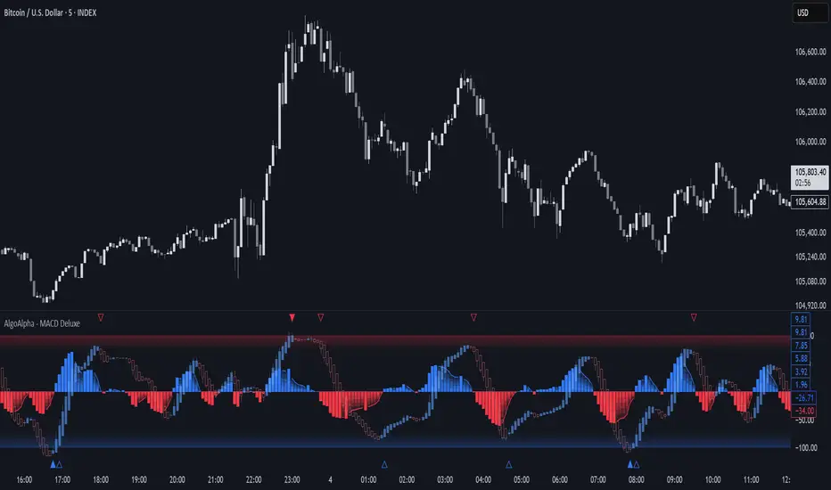
OA - SMESSmart Money Entry Signals (SMES)
The SMES indicator is developed to identify potential turning points in market behavior by analyzing internal price dynamics, rather than relying on external volume or sentiment data. It leverages normalized price movement, directional volatility, and smoothing algorithms to detect potential areas of accumulation or distribution by market participants.
Core Concepts
Smart Money Flow calculation based on normalized price positioning
Directional VHF (Vertical Horizontal Filter) used to enhance signal directionality
Overbought and Oversold regions defined with optional glow visualization
Entry and Exit signals based on dynamic crossovers
Highly customizable input parameters for precision control
Key Inputs
Smart Money Flow Period
Smoothing Period
Price Analysis Length
Fibonacci Lookback Length
Visual toggle options (zones, glow effects, signal display)
Usage
This tool plots the smoothed smart money flow as a standalone oscillator, designed to help traders identify potential momentum shifts or extremes in market sentiment. Entry signals are generated through crossover logic, while optional filters based on price behavior can refine those signals. Exit signals are shown when the smart money line exits extreme regions.
Important Notes
This indicator does not repaint
Works on all timeframes and instruments
Best used as a confirmation tool with other technical frameworks
All calculations are based strictly on price data
Disclaimer
This script is intended for educational purposes only. It does not provide financial advice or guarantee performance. Please do your own research and apply appropriate risk management before making any trading decisions.
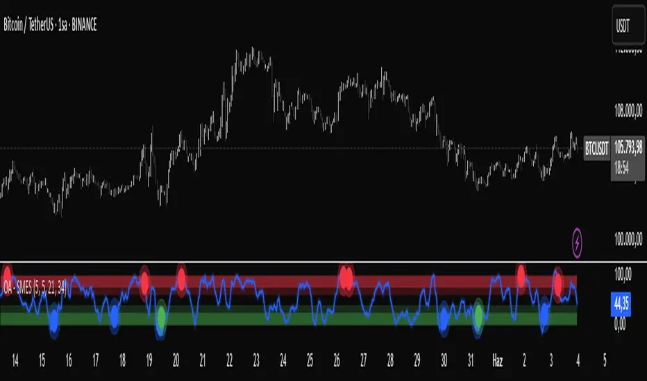
RSI-Adaptive T3 [ChartPrime]The RSI-Adaptive T3 is a precision trend-following tool built around the legendary T3 smoothing algorithm developed by Tim Tillson , designed to enhance responsiveness while reducing lag compared to traditional moving averages. Current implementation takes it a step further by dynamically adapting the smoothing length based on real-time RSI conditions — allowing the T3 to “breathe” with market volatility. This dynamic length makes the curve faster in trending moves and smoother during consolidations.
To help traders visualize volatility and directional momentum, adaptive volatility bands are plotted around the T3 line, with visual crossover markers and a dynamic info panel on the chart. It’s ideal for identifying trend shifts, spotting momentum surges, and adapting strategy execution to the pace of the market.
HOIW IT WORKS
At its core, this indicator fuses two ideas:
The T3 Moving Average — a 6-stage recursively smoothed exponential average created by Tim Tillson , designed to reduce lag without sacrificing smoothness. It uses a volume factor to control curvature.
A Dynamic Length Engine — powered by the RSI. When RSI is low (market oversold), the T3 becomes shorter and more reactive. When RSI is high (overbought), the T3 becomes longer and smoother. This creates a feedback loop between price momentum and trend sensitivity.
// Step 1: Adaptive length via RSI
rsi = ta.rsi(src, rsiLen)
rsi_scale = 1 - rsi / 100
len = math.round(minLen + (maxLen - minLen) * rsi_scale)
pine_ema(src, length) =>
alpha = 2 / (length + 1)
sum = 0.0
sum := na(sum ) ? src : alpha * src + (1 - alpha) * nz(sum )
sum
// Step 2: T3 with adaptive length
e1 = pine_ema(src, len)
e2 = pine_ema(e1, len)
e3 = pine_ema(e2, len)
e4 = pine_ema(e3, len)
e5 = pine_ema(e4, len)
e6 = pine_ema(e5, len)
c1 = -v * v * v
c2 = 3 * v * v + 3 * v * v * v
c3 = -6 * v * v - 3 * v - 3 * v * v * v
c4 = 1 + 3 * v + v * v * v + 3 * v * v
t3 = c1 * e6 + c2 * e5 + c3 * e4 + c4 * e3
The result: an evolving trend line that adapts to market tempo in real-time.
KEY FEATURES
⯁ RSI-Based Adaptive Smoothing
The length of the T3 calculation dynamically adjusts between a Min Length and Max Length , based on the current RSI.
When RSI is low → the T3 shortens, tracking reversals faster.
When RSI is high → the T3 stretches, filtering out noise during euphoria phases.
Displayed length is shown in a floating table, colored on a gradient between min/max values.
⯁ T3 Calculation (Tim Tillson Method)
The script uses a 6-stage EMA cascade with a customizable Volume Factor (v) , as designed by Tillson (1998) .
Formula:
T3 = c1 * e6 + c2 * e5 + c3 * e4 + c4 * e3
This technique gives smoother yet faster curves than EMAs or DEMA/Triple EMA.
⯁ Visual Trend Direction & Transitions
The T3 line changes color dynamically:
Color Up (default: blue) → bullish curvature
Color Down (default: orange) → bearish curvature
Plot fill between T3 and delayed T3 creates a gradient ribbon to show momentum expansion/contraction.
Directional shift markers (“🞛”) are plotted when T3 crosses its own delayed value — helping traders spot trend flips or pullback entries.
⯁ Adaptive Volatility Bands
Optional upper/lower bands are plotted around the T3 line using a user-defined volatility window (default: 100).
Bands widen when volatility rises, and contract during compression — similar to Bollinger logic but centered on the adaptive T3.
Shaded band zones help frame breakout setups or mean-reversion zones.
⯁ Dynamic Info Table
A live stats panel shows:
Current adaptive length
Maximum smoothing (▲ MaxLen)
Minimum smoothing (▼ MinLen)
All values update in real time and are color-coded to match trend direction.
HOW TO USE
Use T3 crossovers to detect trend transitions, especially during periods of volatility compression.
Watch for volatility contraction in the bands — breakouts from narrow band periods often precede trend bursts.
The adaptive smoothing length can also be used to assess current market tempo — tighter = faster; wider = slower.
CONCLUSION
RSI-Adaptive T3 modernizes one of the most elegant smoothing algorithms in technical analysis with intelligent RSI responsiveness and built-in volatility bands. It gives traders a cleaner read on trend health, directional shifts, and expansion dynamics — all in a visually efficient package. Perfect for scalpers, swing traders, and algorithmic modelers alike, it delivers advanced logic in a plug-and-play format.

Strategy Builder With IndicatorsThis strategy script is designed for traders who enjoy building systems using multiple indicators.
Please note: This script does not include any built-in indicators. Instead, it works by referencing the plot outputs of the indicators you’ve already added to your chart.
For example, if you add a MACD and an ATR indicator to your chart, you can assign their plot values as inputs in the settings panel of this strategy.
• MACD as a trigger
• ATR as a filter
How Filters Work
Filters check whether certain conditions are met before a trade can be opened. For instance, if you set a filter like ATR > 30, then no trade will be executed unless that condition is true — even if the trigger fires.
All filters are linked, meaning every active filter must be satisfied for a trade to occur.
How Triggers Work
Triggers are what actually fire a trade signal — such as a moving average crossover or RSI breaking above a specific level. Unlike filters, triggers are independent. Only one active trigger needs to be true for the trade to execute.
Thanks to its modular structure, this strategy can be used with any indicator of your choice.
⸻
Risk Management Features
In the settings, you’ll find flexible options for:
• Stop Loss (SL)
• Trailing Stop Loss (TSL)
• Multi Take-Profit (TP)
These features enhance trade safety and let you tailor your risk management.
SL types available:
• Tick-based SL
• Percent-based SL
• ATR-based SL
Once you select your preferred SL type, you can fine-tune its distance using the offset field.
Trailing SL allows your stop to follow price as it moves in your favor — helping to lock in profits.
Multi-TP lets you take profits at two different levels, helping you secure gains while leaving room for extended moves.
Breakeven option is also available to automatically move your SL to entry after reaching a profit threshold.
⸻
How to Build a Solid Strategy
Let’s break down a good setup into three key components:
1. Trend Filter
Avoid trading against the trend — that’s like swimming against the current.
Use a filter like:
• Supertrend
• Momentum indicators
• Candlestick bias, etc.
Example: In this case, I used Supertrend and filtered for trades only if the price is above the uptrend line.
2. Trigger Condition
Once we confirm the trend is on our side, we need a trigger to execute at the right moment. This can be:
• RSI cross
• Candlestick patterns
• Trendline breaks
• Moving average crossovers, etc.
Example: I used RSI crossing above 50 as the entry trigger.
3. Risk Management
Even in the right trend at the right time — anything can happen. That’s why you should always define Stop Loss and Take Profit levels.
⸻
And there you have it! Your strategy is ready to backtest, refine, and deploy with alerts for live trading.
Questions or suggestions? Feel free to reach out

Supertrend - SSL Strategy with Toggle [AlPashaTrader]📈 Overview of the Supertrend - SSL Strategy with Toggle Indicator
This strategy combines two powerful technical tools—Supertrend and SSL Channel—to deliver precise and reliable trading signals, designed for traders who value confirmation and risk management. 🎯
⚙️ How This Indicator Was Created
The strategy was meticulously crafted to harness the complementary strengths of:
Supertrend Indicator: A trend-following tool based on Average True Range (ATR) and a multiplier factor, it detects bullish or bearish trends by calculating dynamic support and resistance levels. 📊
SSL Channel: A channel indicator built using two Simple Moving Averages (SMA) of the highs and lows over a set period. It cleverly determines trend direction by comparing price action relative to these moving averages. 🔄
These two indicators are merged into one cohesive strategy with an optional toggle feature allowing the trader to choose whether to require confirmation from both indicators before taking a position or to act on signals from either. 🎚️
The script includes user-friendly controls for:
Defining a custom trading date range 📅, useful for backtesting or restricting trading to specific market conditions.
Setting the ATR length and multiplier for Supertrend sensitivity ⚙️.
Adjusting the SSL channel period for responsiveness to price changes ⏱️.
Choosing whether to require dual confirmation (both Supertrend and SSL signals) for more conservative trading or a single indicator trigger for a more aggressive approach 🛡️ vs ⚔️.
🔍 How This Indicator Works
Signal Generation:
Supertrend analyzes market volatility and trend direction, signaling a potential buy when the trend turns bullish 📈 and a sell when bearish 📉.
SSL Channel tracks price relative to its high and low moving averages to identify uptrends and downtrends. A crossover of the SSL Up and SSL Down lines generates buy or sell signals 🔔.
Confirmation Logic:
When confirmation is enabled, the strategy waits for agreement between both indicators before entering a trade ✅, reducing false signals.
When confirmation is disabled, it trades based on signals from either indicator ⚡, allowing more frequent entries but potentially higher risk.
Entry and Exit Rules:
Entry occurs when the indicator(s) signal a new trend direction 🚀 for long, or decline for short.
Exit happens when opposing signals appear 🛑, closing existing positions to lock in profits or cut losses.
Visual Aids:
The SSL Channel lines are plotted directly on the chart with distinct colors to intuitively show trend shifts 🎨.
The system respects the specified date range ⏳, ensuring trades only occur within user-defined periods.
🎯 How to Use This Strategy Effectively
Set Your Preferences: Adjust ATR length, factor, and SSL period to your style. More sensitive? Decrease lengths. Smoother? Increase them ⚙️.
Choose Confirmation Mode: Use the toggle depending on your risk appetite:
Confirmation ON ✅: For conservative traders wanting high-probability setups.
Confirmation OFF ⚡: For aggressive traders who want more signals.
Apply Date Filters: Focus your trading or backtesting on specific periods 📅.
Monitor Entry/Exit Signals: Watch crossovers and Supertrend changes closely 👀.
Risk Management: The strategy uses position sizing as a percentage of equity (default 15%) 💰. Adjust accordingly.
Combine with Other Tools: Enhance results by combining this with volume, price action, or fundamentals 🔧.
📝 Summary
This Supertrend - SSL Strategy with Toggle is a dynamic and flexible trading tool blending volatility-based trend detection with moving-average channel insights. It empowers traders to customize confirmation strictness, control trading periods, and efficiently capture trending opportunities while managing risk smartly.
By integrating proven indicators in a user-friendly, visually intuitive package, this strategy stands as a sophisticated tool suitable for various markets and trading styles. 🚀📊
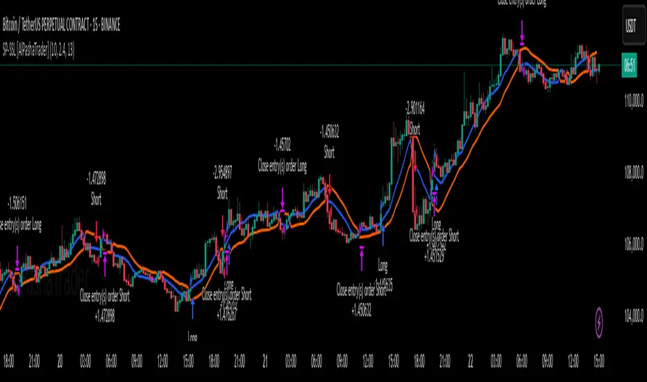
PhenLabs - Market Fluid Dynamics📊 Market Fluid Dynamics -
Version: PineScript™ v6
📌 Description
The Market Fluid Dynamics - Phen indicator is a new thinking regarding market analysis by modeling price action, volume, and volatility using a fluid system. It attempts to offer traders control over more profound market forces, such as momentum (speed), resistance (thickness), and buying/selling pressure. By visualizing such dynamics, the script allows the traders to decide on the prevailing market flow, its power, likely continuations, and zones of calmness and chaos, and thereby allows improved decision-making.
This measure avoids the usual difficulty of reconciling multiple, often contradictory, market indications by including them within a single overarching model. It moves beyond traditional binary indicators by providing a multi-dimensional view of market behavior, employing fluid dynamic analogs to describe complex interactions in an accessible manner.
🚀 Points of Innovation
Integrated Fluid Dynamics Model: Combines velocity, viscosity, pressure, and turbulence into a single indicator.
Normalized Metrics: Uses ATR and other normalization techniques for consistent readings across different assets and timeframes.
Dynamic Flow Visualization: Main flow line changes color and intensity based on direction and strength.
Turbulence Background: Visually represents market stability with a gradient background, from calm to turbulent.
Comprehensive Dashboard: Provides an at-a-glance summary of key fluid dynamic metrics.
Multi-Layer Smoothing: Employs several layers of EMA smoothing for a clearer, more responsive main flow line.
🔧 Core Components
Velocity Component: Measures price momentum (first derivative of price), normalized by ATR. It indicates the speed and direction of price changes.
Viscosity Component: Represents market resistance to price changes, derived from ATR relative to its historical average. Higher viscosity suggests it’s harder for prices to move.
Pressure Component: Quantifies the force created by volume and price range (close - open), normalized by ATR. It reflects buying or selling pressure.
Turbulence Detection: Calculates a Reynolds number equivalent to identify market stability, ranging from laminar (stable) to turbulent (chaotic).
Main Flow Indicator: Combines the above components, applying sensitivity and smoothing, to generate a primary signal of market direction and strength.
🔥 Key Features
Advanced Smoothing Algorithm: Utilizes multiple EMA layers on the raw flow calculation for a fluid and responsive main flow line, reducing noise while maintaining sensitivity.
Gradient Flow Coloring: The main flow line dynamically changes color from light to deep blue for bullish flow and light to deep red for bearish flow, with intensity reflecting flow strength. This provides an immediate visual cue of market sentiment and momentum.
Turbulence Level Background: The chart background changes color based on calculated turbulence (from calm gray to vibrant orange), offering an intuitive understanding of market stability and potential for erratic price action.
Informative Dashboard: A customizable on-screen table displays critical metrics like Flow State, Flow Strength, Market Viscosity, Turbulence, Pressure Force, Flow Acceleration, and Flow Continuity, allowing traders to quickly assess current market conditions.
Configurable Lookback and Sensitivity: Users can adjust the base lookback period for calculations and the sensitivity of the flow to viscosity, tailoring the indicator to different trading styles and market conditions.
Alert Conditions: Pre-defined alerts for flow direction changes (positive/negative crossover of zero line) and detection of high turbulence states.
🎨 Visualization
Main Flow Line: A smoothed line plotted below the main chart, colored blue for bullish flow and red for bearish flow. The intensity of the color (light to dark) indicates the strength of the flow. This line crossing the zero line can signal a change in market direction.
Zero Line: A dotted horizontal line at the zero level, serving as a baseline to gauge whether the market flow is positive (bullish) or negative (bearish).
Turbulence Background: The indicator pane’s background color changes based on the calculated turbulence level. A calm, almost transparent gray indicates low turbulence (laminar flow), while a more vibrant, semi-transparent orange signifies high turbulence. This helps traders visually assess market stability.
Dashboard Table: An optional table displayed on the chart, showing key metrics like ‘Flow State’, ‘Flow Strength’, ‘Market Viscosity’, ‘Turbulence’, ‘Pressure Force’, ‘Flow Acceleration’, and ‘Flow Continuity’ with their current values and qualitative descriptions (e.g., ‘Bullish Flow’, ‘Laminar (Stable)’).
📖 Usage Guidelines
Setting Categories
Show Dashboard - Default: true; Range: true/false; Description: Toggles the visibility of the Market Fluid Dynamics dashboard on the chart. Enable to see key metrics at a glance.
Base Lookback Period - Default: 14; Range: 5 - (no upper limit, practical limits apply); Description: Sets the primary lookback period for core calculations like velocity, ATR, and volume SMA. Shorter periods make the indicator more sensitive to recent price action, while longer periods provide a smoother, slower signal.
Flow Sensitivity - Default: 0.5; Range: 0.1 - 1.0 (step 0.1); Description: Adjusts how much the market viscosity dampens the raw flow. A lower value means viscosity has less impact (flow is more sensitive to raw velocity/pressure), while a higher value means viscosity has a greater dampening effect.
Flow Smoothing - Default: 5; Range: 1 - 20; Description: Controls the length of the EMA smoothing applied to the main flow line. Higher values result in a smoother flow line but with more lag; lower values make it more responsive but potentially noisier.
Dashboard Position - Default: ‘Top Right’; Range: ‘Top Right’, ‘Top Left’, ‘Bottom Right’, ‘Bottom Left’, ‘Middle Right’, ‘Middle Left’; Description: Determines the placement of the dashboard on the chart.
Header Size - Default: ‘Normal’; Range: ‘Tiny’, ‘Small’, ‘Normal’, ‘Large’, ‘Huge’; Description: Sets the text size for the dashboard header.
Values Size - Default: ‘Small’; Range: ‘Tiny’, ‘Small’, ‘Normal’, ‘Large’; Description: Sets the text size for the metric values in the dashboard.
✅ Best Use Cases
Trend Identification: Identifying the dominant market flow (bullish or bearish) and its strength to trade in the direction of the prevailing trend.
Momentum Confirmation: Using the flow strength and acceleration to confirm the conviction behind price movements.
Volatility Assessment: Utilizing the turbulence metric to gauge market stability, helping to adjust position sizing or avoid choppy conditions.
Reversal Spotting: Watching for divergences between price and flow, or crossovers of the main flow line above/below the zero line, as potential reversal signals, especially when combined with changes in pressure or viscosity.
Swing Trading: Leveraging the smoothed flow line to capture medium-term market swings, entering when flow aligns with the desired trade direction and exiting when flow weakens or reverses.
Intraday Scalping: Using shorter lookback periods and higher sensitivity to identify quick shifts in flow and turbulence for short-term trading opportunities, particularly in liquid markets.
⚠️ Limitations
Lagging Nature: Like many indicators based on moving averages and lookback periods, the main flow line can lag behind rapid price changes, potentially leading to delayed signals.
Whipsaws in Ranging Markets: During periods of low volatility or sideways price action (high viscosity, low flow strength), the indicator might produce frequent buy/sell signals (whipsaws) as the flow oscillates around the zero line.
Not a Standalone System: While comprehensive, it should be used in conjunction with other forms of analysis (e.g., price action, support/resistance levels, other indicators) and not as a sole basis for trading decisions.
Subjectivity in Interpretation: While the dashboard provides quantitative values, the interpretation of “strong” flow, “high” turbulence, or “significant” acceleration can still have a subjective element depending on the trader’s strategy and risk tolerance.
💡 What Makes This Unique
Fluid Dynamics Analogy: Its core strength lies in translating complex market interactions into an intuitive fluid dynamics framework, making concepts like momentum, resistance, and pressure easier to visualize and understand.
Market View: Instead of focusing on a single aspect (like just momentum or just volatility), it integrates multiple factors (velocity, viscosity, pressure, turbulence) to provide a more comprehensive picture of market conditions.
Adaptive Visualization: The dynamic coloring of the flow line and the turbulence background provide immediate, adaptive visual feedback that changes with market conditions.
🔬 How It Works
Price Velocity Calculation: The indicator first calculates price velocity by measuring the rate of change of the closing price over a given ‘lookback’ period. The raw velocity is then normalized by the Average True Range (ATR) of the same lookback period. Normalization enables comparison of momentum between assets or timeframes by scaling for volatility. This is the direction and speed of initial price movement.
Viscosity Calculation: Market ‘viscosity’ or resistance to price movement is determined by looking at the current ATR relative to its longer-term average (SMA of ATR over lookback * 2). The further the current ATR is above its average, the lower the viscosity (less resistance to price movement), and vice-versa. The script inverts this relationship and bounds it so that rising viscosity means more resistance.
Pressure Force Measurement: A ‘pressure’ variable is calculated as a function of the ratio of current volume to its simple moving average, multiplied by the price range (close - open) and normalized by ATR. This is designed to measure the force behind price movement created by volume and intraday price thrusts. This pressure is smoothed by an EMA.
Turbulence State Evaluation: A equivalent ‘Reynolds number’ is calculated by dividing the absolute normalized velocity by the viscosity. This is the proclivity of the market to move in a chaotic or orderly fashion. This ‘reynoldsValue’ is smoothed with an EMA to get the ‘turbulenceState’, which indicates if the market is laminar (stable), transitional, or turbulent.
Main Flow Derivation: The ‘rawFlow’ is calculated by taking the normalized velocity, dampening its impact based on the ‘viscosity’ and user-input ‘sensitivity’, and orienting it by the sign of the smoothed ‘pressureSmooth’. The ‘rawFlow’ is then put through multiple layers of exponential moving average (EMA) smoothing (with ‘smoothingLength’ and derived values) to reach the final ‘mainFlow’ line. The extensive smoothing is designed to give a smooth and clear visualization of the overall market direction and magnitude.
Dashboard Metrics Compilation: Additional metrics like flow acceleration (derivative of mainFlow), and flow continuity (correlation between close and volume) are calculated. All primary components (Flow State, Strength, Viscosity, Turbulence, Pressure, Acceleration, Continuity) are then presented in a user-configurable dashboard for ease of monitoring.
💡 Note:
The “Market Fluid Dynamics - Phen” indicator is designed to offer a unique perspective on market behavior by applying principles from fluid dynamics. It’s most effective when used to understand the underlying forces driving price rather than as a direct buy/sell signal generator in isolation. Experiment with the settings, particularly the ‘Base Lookback Period’, ‘Flow Sensitivity’, and ‘Flow Smoothing’, to find what best suits your trading style and the specific asset you are analyzing. Always combine its insights with robust risk management practices.