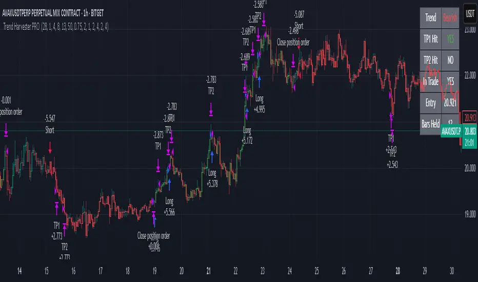
Trend Harvester PRO Trend Harvester PRO – Adaptive Trend-Following Strategy for Crypto
Trend Harvester PRO is a fully systematic trend-following strategy built for cryptocurrency markets on intraday timeframes — particularly optimized for the 1-hour chart. The script combines ZLEMA-based trend tracking, momentum confirmation, and a volatility-aware filter to detect high-probability directional moves with clarity and precision.
This is not a mashup of random indicators — each component serves a specific purpose in validating trends, avoiding choppy zones, and timing entries responsibly.
🔍 Strategy Logic Overview
The core objective is to detect sustainable, real-time trends and exit with multi-stage profit targets. To do this, the script uses several layers of confirmation:
1. 📊 ZLEMA Trend Engine (Zero Lag EMA)
This is the backbone of the strategy.
ZLEMA (Zero-Lag EMA) is a moving average that minimizes lag by adjusting for past data offset.
The strategy uses a fast ZLEMA and a slow ZLEMA, combined with a slope calculation, to assess the current trend.
When:
Fast ZLEMA > Slow ZLEMA
The ZLEMA is rising (positive slope)
→ The market is considered in an uptrend.
Conversely, if:
Fast ZLEMA < Slow ZLEMA
The slope is negative
→ The market is considered in a downtrend.
This setup detects not just direction, but also whether the trend has meaningful acceleration.
2. ⚡ Momentum Confirmation
Trend direction alone isn’t enough — we also need momentum agreement.
The script calculates a smoothed Rate of Change (ROC) to evaluate if momentum supports the direction of the ZLEMA trend.
For long trades: ROC must be positive
For short trades: ROC must be negative
This prevents taking trades where price is crossing moving averages but lacks follow-through power.
3. 🌪️ Volatility Filter
Choppy markets are common in crypto. To reduce false signals:
The script compares short-term volatility (10-bar standard deviation of price changes) to longer-term volatility.
If the ratio is too high (i.e., short-term volatility is spiking), the strategy avoids entry.
This ensures trades are only taken when the market is relatively calm and directional — avoiding false breakouts.
4. 🧠 Confirmation Bars + Trend State
Signals only trigger after a certain number of consecutive bars confirm trend direction (confirmBars).
This prevents reacting to just 1 candle and requires consistent evidence of trend.
A state machine is used to track current trend status:
+1 = confirmed uptrend
-1 = confirmed downtrend
0 = neutral / no trade
This trend state changes only after all conditions are met and confirmation bars pass.
5. 🧊 Cooldown Enforcement
After a trade exits (from TP or a trend reversal), the strategy enforces a cooldown period before new entries are allowed. This:
Prevents back-to-back entries on trend flips
Reduces overtrading
Helps avoid whipsaws or same-bar reversal trades
6. 🎯 Multi-Level Take Profits (TP1 & TP2)
Once a trade is entered:
Two limit exits are set automatically:
TP1: Closes 50% of the position at a configurable profit level
TP2: Closes the remaining 50%
If the trend weakens before TP2 is reached, the position is closed early.
Both long and short trades use the same logic, with user-defined percentages.
This system allows for partial profit-taking while keeping a portion of the trade running.
7. 🧾 Built-in Dashboard
The script includes a real-time dashboard showing:
Trend direction: Bullish, Bearish, or Neutral
Whether TP1 / TP2 was hit
Entry price
If currently in a trade
How many bars the trade has been open
This helps monitor strategy performance at a glance without needing extra labels.
8. 🔔 Webhook-Compatible Alerts
The strategy includes custom alerts that can be used for:
Long and Short entries
TP1 and TP2 hits
Exiting trades
These can be integrated into automated bot systems or used manually.
🔒 Non-Repainting Logic
The strategy uses only confirmed bar data (i.e., values from closed bars).
There are no repainting indicators.
Entries and exits are placed using strategy.entry and strategy.exit on confirmed conditions.
✅ How to Use It
Apply the strategy to 1H altcoin charts (BTC, ETH, SOL, etc.).
Tune the TP percentages (longTP1Pct, longTP2Pct, etc.) based on volatility.
Use the dashboard to monitor trend state and trade progress.
Combine with additional tools (like support/resistance or volume) for higher confluence.
Use the date filter to run backtests over defined periods.
⚠️ Risk Management Notice
This strategy does not include stop losses by default. It is designed to exit based on trend reversal or take-profit limits.
Always backtest thoroughly and use realistic sizing.
Do not risk more than 5–10% of your account on any trade.
Past results do not guarantee future performance. This tool is for educational and research purposes.
🧬 What Makes This Original
Trend Harvester PRO was built from scratch with tightly integrated logic:
ZLEMA tracks early trend direction with low lag
ROC confirms momentum in the same direction
Volatility filter avoids false setups
Multi-bar confirmation and cooldown logic control trade pacing
Dual TP exits manage partial profit-taking
A live dashboard makes real-time tracking intuitive
Unlike mashups of indicators with no synergy, each component here directly supports the quality of trade decisions, and the logic is modular, transparent, and non-repainting.
Pesquisar nos scripts por "bot"
SmartScale Envelope DCA This is a Dollar-Cost Averaging (DCA) long strategy that buys when price dips below a moving average envelope and adds to the position in a stepwise, risk-controlled way. It uses up to 8 buy-ins, applies a cooldown between entries, and exits based on either a take profit from average entry price or a stop loss. Backtest range limits trades to the last 365 days for backtest control.
All input settings can and should be adjusted to the chart, as volatility in price action varies. Simply go into the inputs settings, and start from the top and move down to get better backtest results. Moving from the top down has been proven to give the best results. Then, move to properties and set your order size, pyramiding, and so on. It may be necessary to then fine tune your adjustments a second time to dial it in.
Works well on 1 hour time frames and in volatility.
Happy Trading!

Prime Trend ReactorIntroduction
Prime Trend Reactor is an advanced crypto trend-following strategy designed to deliver precision entries and exits based on a multi-factor trend consensus system.
It combines price action, adaptive moving averages, momentum oscillators, volume analysis, volatility signals, and higher timeframe trend confirmation into a non-repainting, fully systematic approach.
This strategy is original: it builds a unique trend detection matrix by blending multiple forms of price-derived signals through weighted scoring, rather than simply stacking indicators.
It is not a mashup of public indicators — it is engineered from the ground up using custom formulas and strict non-repainting design.
It is optimized for 1-hour crypto charts but can be used across any asset or timeframe.
⚙️ Core Components
Prime Trend Reactor integrates the following custom components:
1. Moving Averages System
Fast EMA (8), Medium EMA (21), Slow EMA (50), Trend EMA (200).
Detects short-term, medium-term, and long-term trend structures.
EMA alignment is scored as part of the trend consensus system.
2. Momentum Oscillators
RSI (Relative Strength Index) with Smoothing.
RMI (Relative Momentum Index) custom-calculated.
Confirms price momentum behavior aligned with trend.
3. Volume Analysis
CMF (Chaikin Money Flow) for accumulation/distribution pressure.
OBV (On Balance Volume) EMA Cross for volume flow confirmation.
4. Volatility and Price Structure
Vortex Indicator (VI+ and VI-) for trend strength and directional bias.
Mean-Extreme Price Engine blends closing price with extremes (high/low) based on user-defined ratio.
5. Structure Breakout Detection
Detects structure breaks based on highest high/lowest low pivots.
Adds weight to trend strength on fresh breakouts.
6. Higher Timeframe Confirmation (HTF)
Uses higher timeframe EMAs and close to confirm macro-trend direction.
Smartly pulls HTF data with barmerge.lookahead_off to avoid repainting.
🔥 Entry and Exit Logic
Long Entry: Triggered when multi-factor trend consensus turns strongly bullish.
Short Entry: Triggered when consensus flips strongly bearish.
Take Profits (TP1/TP2):
TP1: Partial 50% profit at small target.
TP2: Full 100% close at larger target.
Exit on Trend Reversal:
If trend consensus reverses before hitting TP2, the strategy exits early to protect capital.
TP Hits and Trend Reversals fire real-time webhook-compatible alerts.
🧩 Trend Consensus Matrix (Original Concept)
Instead of relying on a single indicator, Prime Trend Reactor calculates a weighted score using:
EMA Alignment
Momentum Oscillators (RSI + RMI)
Volume Analysis
Volatility (Vortex)
Higher Timeframe Bias
Each component adds a weighted contribution to the final trend strength score.
Only when the weighted score exceeds a user-defined threshold does the system allow entries.
This multi-dimensional scoring system is original and engineered specifically to avoid noisy or lagging traditional signals.
📈 Visualization and Dashboard
Custom EMA Clouds dynamically fill between Fast/Medium EMAs.
Colored Candles show real-time trend direction.
Dynamic Dashboard displays:
Current Position (Long/Short/Flat)
Entry Price
TP1 and TP2 Hit Status
Bars Since Entry
Win Rate (%)
Profit Factor
Current Trend Signal
Consensus Score (%)
🛡️ Non-Repainting Design
All trend calculations are based on current and confirmed past data.
HTF confirmations use barmerge.lookahead_off.
No same-bar entries and exits — enforced logic prevents overlap.
No lookahead bias.
Strict variable handling ensures confirmed-only trend state transitions.
✅ 100% TradingView-approved non-repainting behavior.
📣 Alerts and Webhooks
This strategy includes full TradingView webhook support:
Long/Short Entries
TP1 Hit (Partial Exit)
TP2 Hit (Full Exit)
Exit on Trend Reversal
All alerts use constant-string JSON formatting compliant with TradingView multi-exchange bots:
📜 TradingView Mandatory Disclaimer
This strategy is a tool to assist in market analysis. It does not guarantee profitability. Trading financial markets involves risk. You are solely responsible for your trading decisions. Past performance does not guarantee future results.

Sniper Core XT🔫 SNIPER CORE XT — ZLEMA-Based Trend + Momentum Strategy for Crypto
⚙️ How It Works (What Makes It Unique):
Sniper Core XT is a fully automated, non-repainting crypto strategy that combines a purpose-built trend detection system with volatility, volume, and momentum confirmation. It is designed from scratch in Pine Script v5 and optimized for bot deployment, copy trading, or semi-manual execution on the 1H timeframe.
Unlike a simple indicator mashup, this strategy builds its logic around one core component — ZLEMA (Zero-Lag Exponential Moving Average) — and then selectively adds only supporting filters that refine trend detection and execution logic.
🧠 Core Logic & Components:
ZLEMA Trend Engine:
The main trend signal comes from a fast vs. slow ZLEMA crossover. ZLEMA is chosen for its responsiveness and minimal lag, giving traders earlier entries without the noise of standard EMAs.
Vortex Direction & Strength Filter:
Uses Vortex Indicator internals to measure directional conviction. The strategy only enters if the vortex aligns with ZLEMA direction and shows minimum strength based on a customizable threshold.
Volume Confirmation via ZLEMA of Volume:
Filters out weak moves by confirming that current volume exceeds the ZLEMA-smoothed average of volume, creating adaptive volume thresholds.
Adaptive Momentum Filter:
Momentum is measured by a normalized rate-of-change adjusted for volatility (ATR). This helps avoid flat market entries and overextends.
Hardcoded Stop Loss (2%) and Dual TP:
TP1: 50% profit scale-out
TP2: Full closure
Stop loss exits on bar close, not using built-in SL/TP orders — this allows reentry if conditions remain favorable.
Real-Time Non-Canvas Dashboard:
A lightweight table shows entry price, trend direction, TP1/TP2/SL hit status, and bars in trade — all configurable for screen position and font size.
One-Bar Cooldown Mechanism:
Prevents entering and exiting on the same bar. Reinforces realistic execution logic and avoids repaint artifacts.
🧪 Strategy Use & Applications:
Designed for 1H trading of trending crypto pairs
Works well in medium-to-high volatility conditions
Fully supports multi-exchange alerts for integration with:
WunderTrading
3Commas
Cornix
PineConnector
🛡️ Strategy Style:
Feature Value
Repainting ❌ Never
Entry Cooldown ✅ 1-Bar
SL Handling ✅ 2% from entry (hardcoded)
TP1/TP2 ✅ Built-in (limit orders)
Alert Compatible ✅ Fully supported
Timeframe 🕒 1H recommended
⚠️ Disclaimer:
This is not financial advice. All signals are based on historical logic and may differ in live markets. Always use proper position sizing and risk management.
📌 Publishing Notes
This strategy is original and built from scratch. While it uses ZLEMA and Vortex as components, all logic — including volume filters, momentum filters, TP/SL logic, and dashboard — has been custom-coded and tested specifically for crypto trend-following on the 1H timeframe.

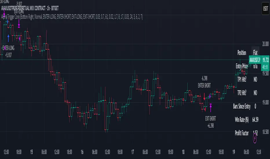
Alpha Trigger CoreAlpha Trigger Core — Trend Momentum Strategy with Dual Take Profit System
Alpha Trigger Core is a precision-engineered trend-following strategy developed for crypto and altcoin markets. Unlike simple indicator mashups, this system was built from the ground up with a specific logic framework that integrates trend, momentum, volatility, and structure validation into a single unified strategy.
It is not a random combination of indicators, but rather a coordinated system of filters that work together to increase signal quality and minimize false positives. This makes it especially effective on trending assets like BTC, ETH, AVAX, and SOL on the 1-hour chart.
🔍 How It Works
This strategy fuses multiple advanced filters into a cohesive signal engine:
🔹 Trend Identification
A hybrid model combining:
Kalman Filter — Smooths price noise with predictive tracking.
SuperTrend Overlay — Confirms directional bias using ATR.
ZLEMA Envelope — Defines dynamic upper/lower bounds based on price velocity.
🔹 Momentum Filter
Uses a ZLEMA-smoothed CCI to identify accelerating moves.
Long entries require a rising 3-bar CCI sequence.
Short entries require a falling 3-bar CCI sequence.
🔹 Volatility Strength Filter (Vortex Indicator)
Validates entries only when Vortex Diff exceeds a customizable threshold.
Prevents low-volatility "chop zone" trades.
🔹 Wick Trap Filter
Filters out false breakouts driven by liquidity wicks.
Validates that body structure supports the breakout.
📈 Entry & Exit Logic
Long Entry: All trend, momentum, volatility filters must align bullishly and wick traps must be absent.
Short Entry: All filters must align bearishly, with no wick rejection.
Early Exit: Uses ZLEMA slope crossover to exit before a full trend reversal is confirmed.
🎯 Take Profit System
TP1: Takes 50% profit at a user-defined % target.
TP2: Closes remaining 100% at second target.
Cooldown: Prevents immediate reentry and ensures clean position transitions.
📊 Real-Time Strategy Dashboard
Tracks and displays:
Position status (Long, Short, Flat)
Entry Price
TP1/TP2 Hit status
Win Rate (%)
Profit Factor
Bars Since Entry
Fully customizable position & font size
🤖 Bot-Ready Multi-Exchange Alerts
Compatible with WonderTrading, 3Commas, Binance, Bybit, and more.
Customizable comment= tags for entry, exit, TP1, and TP2.
Fully alert-compatible for webhook integrations.
📌 Suggested Use
Best used on trending crypto pairs with moderate-to-high volatility. Recommended on the 1H timeframe for altcoins and majors. Can be used for manual confirmation or automated trading.
🔒 Script Transparency
This is a closed-source script. However, the description above provides a transparent breakdown of the strategy’s core logic, filters, and execution model — ensuring compliance with TradingView’s publishing guidelines.
⚠️ Trading Disclaimer
This script is for educational purposes only and is not financial advice. Always conduct your own analysis before making investment decisions. Past performance does not guarantee future results. Use this strategy at your own risk.
IronBot v4IronBot v4 – Trading Strategy Overview
1. Quick Context
IronBot v4 is a trading strategy designed for users who want a simple yet effective approach to reading the markets. It uses a combination of Fibonacci retracement levels, custom logic triggers, and innovative modules (EMA validation, Iron Impulse Shield and Iron Auto Volume Detector) to identify potential entry and exit points, strengthening the strategy’s detection of sudden market volatility or shifts in trading volume.
2. Theoretical Details
Fibonacci Analysis
The script identifies recent market highs and lows, then calculates key Fibonacci levels (high- and low-based). These levels can help confirm potential reversals or trends.
EMA Option
When enabled, the exponential moving average (EMA) offers additional validation for trade entries. If the current price remains above a certain EMA threshold, long positions may be favored; conversely, if it stays below the EMA, short positions may be initiated.
IIS (Iron Impulse Shield)
IIS helps to filter out risky trades by measuring recent price shocks or surges. If an extreme movement is detected, the strategy may temporarily disable longs or shorts to avoid false signals.
IAVD (Iron Auto Volume Detector)
This functionality automatically detects the average market volume over a defined period (regardless of the market, since it relies on real data). When entering a position, it ensures that overall volume is high enough to confirm a genuinely active, robust market. By providing an additional filter, it can strengthen the decision-making process whenever the market’s participation level is in question.
Panel
IronBot v4 displays a real-time backtest panel that summarizes the selected configuration (including the current pair, analysis window, enabled filters), as well as showing net profit, applicable exchange fees, country taxes, and the final net balance. This gives traders an immediate overview of strategy performance and risk metrics.
What Pinescript Adds Visually
The script plots:
Fibonacci levels (highlighting potential reversal zones)
Trend lines indicating bullish (green) or bearish (red) lean
Optional EMA line
Optional Fibonacci forecast lines for anticipating future moves
Automatic labeling of entry, take-profit, and stop-loss levels, indicating the profit percentage of each trade.
3. Explanation of Inputs
The strategy exposes multiple inputs that can be toggled or configured by the user:
Analysis Window : Dictates how many bars to consider for high/low calculations and the fib retracement thresholds.
TRADES
Display TP/SL: For displaying Take profits and Stop loss.
Display Forecast: When enabled, this feature calculates and projects possible future Fibonacci retracements using historical data, helping traders anticipate potential upcoming trade setups.
Leverage: Only used for the Panel and not for trades. Lets you amplify your position size; higher leverage increases potential gains but also heightens risk. TradingView strategy is using properties for doing this.
Exchange Maker Fees & Exchange Taker Fees: Only used for the Panel and not for trades. Define the percentage cost applied by your exchange for maker and taker trades, respectively. These fees are accounted for in final profit calculations of the Panel.
Country Tax: Only used for the Panel and not for trades. Specifies a tax percentage to be deducted from net profits.
STOP LOSS and TAKE PROFITS
Stop-Loss & Take-Profit Parameters: Controls the percentage distances at which the strategy will exit positions. Additionally, you can configure up to four distinct take-profit levels (TP1 through TP4). Each level should be higher target than the previous one, and you can assign a specific percentage of the total position to close at each TP, ensuring the sum equals 100%. A break-even feature is also available when multiple TPs are used.
EMA
EMA (Exponential Moving Average) Option: When enabled, the strategy opens long trades only if the current price is above the specified EMA length, and opens short trades only if it is below that threshold.
PANELS
Show Panel: For displaying the backtest integrated panel.
IRON IMPULSE SHIELD (IIS)
IIS (Iron Impulse Shield) Option: When enabled, IIS continuously monitors recent price volatility depending on the analysis window set. If the market experiences an extreme surge or drop beyond a specified threshold, IIS temporarily blocks new long or short positions.
IRON AUTO VOLUME DETECTOR (IAVD)
IAVD (Iron Auto Volume Detector) Option: When enabled, it continuously measures the average market volume over a special period, irrespective of the specific trading pair. This ensures that IronBot v4 focuses on markets with robust participation, reducing the likelihood of entering trades during low-liquidity conditions.
By changing these values, IronBot v4 reacts differently to market structure and risk management requirements. Stop-loss and take-profit levels will adjust accordingly, while advanced filters (like EMA or IIS) influence when trades can open.
4. TradingView Strategy Properties
IronBot v4 uses the built-in TradingView “strategy” functionality. In particular:
Order Placement: The code calls strategy.entry() and strategy.close() for direct orders, ensuring signals are sent immediately (no limit orders are used). This helps connect with exchange signal bots for automated execution.
Initial Capital: The code uses initial capital defined in properties for calculating Net balance in the integrated panel.
On bar close: This strategy fill orders on bar close.
Pyramiding: This strategy can take only 1 successive trade in the same direction
Be careful to configure your leverage input depending on your strategy properties.
5. Visualization
5. Purpose & Disclaimer
This script is for educational purposes only and does not constitute financial advice. Past performance does not guarantee future results. Always confirm your own risk tolerance and consult a financial professional before placing live trades. Trading leveraged products can involve substantial risk of loss.

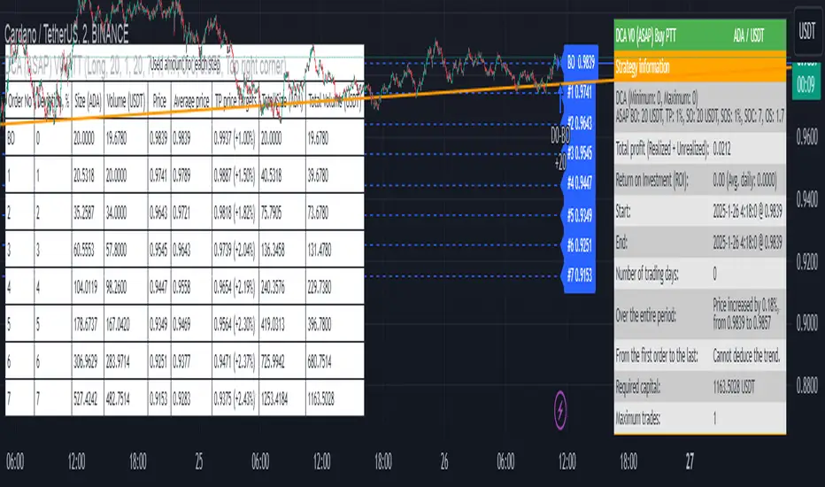
DCA (ASAP) V0 PTTScript Name: DCA (ASAP) V0 PTT
Detailed Description:
This script implements the Dollar-Cost Averaging (DCA) strategy, allowing you to automatically manage buy/sell orders safely and efficiently. Below are the key features of this script:
1. Purpose and Operation:
o Supports both Long and Short trading modes.
o Designed to optimize profitability using the DCA method, where Safety Orders are triggered when the price moves against the predicted direction.
o Helps users maintain their Target Profit in various market conditions.
2. Main Features:
o Automatic Order Placement: The initial Base Order is opened as soon as no active order exists.
o Safety Order Management: Safety Orders are automatically placed when the price moves against the initial order. The volume and distance of these orders are customizable.
o Order Closing: Orders are closed upon reaching the Target Profit, accounting for transaction fees.
o Detailed Information Display: Displays open orders, trading statistics, and performance metrics directly on the chart.
3. Customizable Parameters:
o Base Order Size: The size of the initial order.
o Target Profit (%): Target profit as a percentage of the total order volume.
o Safety Order Size: The size of each Safety Order.
o Price Deviation (%): The percentage distance between consecutive Safety Orders.
o Safety Order Volume Scale: The scaling factor for increasing the volume of subsequent Safety Orders.
o Max Safety Orders: The maximum number of Safety Orders allowed per deal.
4. Unique Features:
o Backtest Range Support: Enables you to limit backtesting to a specific time range of interest.
o Comprehensive Statistics: Displays detailed tables including open trades, pending orders, ROI, trading days, and realized profit.
o Integrated Trading Fees: Includes transaction fees in profit calculations for precise results.
5. Usage Instructions:
o Select the trading mode (Long or Short) from the "Strategy" input.
o Customize parameters such as Base Order, Safety Order, and Target Profit according to your requirements and the asset being traded.
o Monitor the performance of the strategy through the displayed information tables.
Notes:
• This script does not disclose detailed calculation logic but provides an overview of the concepts and usage.
• Designed for trading on exchanges that support margin or spot trading.
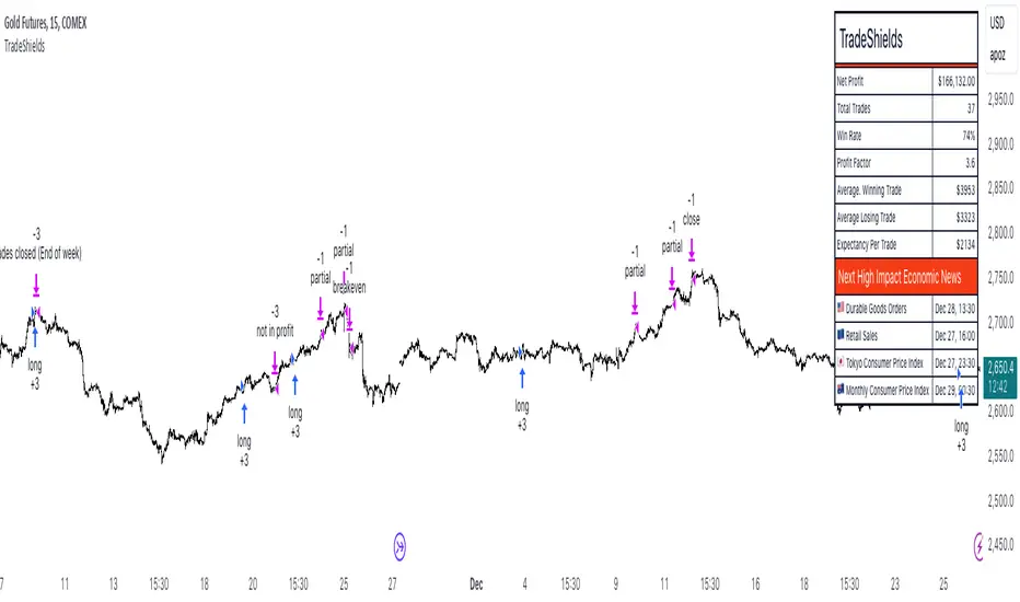
TradeShields Strategy Builder🛡 WHAT IS TRADESHIELDS?
This no-code strategy builder is designed for traders on TradingView, offering an intuitive platform to create, backtest, and automate trading strategies. While identifying signals is often straightforward, the real challenge in trading lies in managing risk and knowing when not to trade. It equips users with advanced tools to address this challenge, promoting disciplined decision-making and structured trading practices.
This is not just a collection of indicators but a comprehensive toolkit that helps identify high-quality opportunities while placing risk management at the core of every strategy. By integrating customizable filters, robust controls, and automation capabilities, it empowers traders to align their strategies with their unique objectives and risk tolerance.
_____________________________________
🛡 THE GOAL: SHIELD YOUR STRATEGY
The mission is simple: to shield your strategy from bad trades . Whether you're a seasoned trader or just starting, the hardest part of trading isn’t finding signals—it’s avoiding trades that can harm your account. This framework prioritizes quality over quantity , helping filter out suboptimal setups and encouraging disciplined execution.
With tools to manage risk, avoid overtrading, and adapt to changing market conditions, it protects your strategy against impulsive decisions and market volatility.
_____________________________________
🛡 HOW TO USE IT
1. Apply Higher Timeframe Filters
Begin by analyzing broader market trends using tools like the 200 EMA, Ichimoku Cloud, or Supertrend on higher timeframes (e.g., daily or 4-hour charts).
- Example: Ensure the price is above the 200 EMA on the daily chart for long trades or below it for short trades.
2. Identify the Appropriate Entry Signal
Choose an entry signal that aligns with your model and the asset you're trading. Options include:
Supertrend changes for trend reversals.
Bollinger Band touches for mean-reversion trades.
RSI strength/weakness for overbought or oversold conditions.
Breakouts of key levels (e.g., daily or weekly highs/lows) for momentum trades.
MACD and TSI flips.
3. Determine Take-Profit and Stop-Loss Levels
Set clear exit strategies to protect your capital and lock in profits:
Use single, dual, or triple take-profit levels based on percentages or price levels.
Choose a stop-loss type, such as fixed percentage, ATR-based, or trailing stops.
Optionally, set breakeven adjustments after hitting your first take-profit target.
4. Apply Risk Management Filters
Incorporate risk controls to ensure disciplined execution:
Limit the number of trades per day, week, or month to avoid overtrading.
Use time-based filters to trade during specific sessions or custom windows.
Avoid trading around high-impact news events with region-specific filters.
5. Automate and Execute
Leverage the advanced automation features to streamline execution. Alerts are tailored specifically for each supported platform, ensuring seamless integration with tools like PineConnector, 3Commas, Zapier, and more.
_____________________________________
🛡 CORE FOCUS: RISK MANAGEMENT, AUTOMATION, AND DISCIPLINED TRADING
This builder emphasizes quality over quantity, encouraging traders to approach markets with structure and control. Its innovative tools for risk management and automation help optimize performance while reducing effort, fostering consistency and long-term success.
_____________________________________
🛡 KEY FEATURES
General Settings
Theme Customization : Light and dark themes for a tailored interface.
Timezone Adjustment : Align session times and news schedules with your local timezone.
Position Sizing : Define lot sizes to manage risk effectively.
Directional Control : Choose between long-only, short-only, or both directions for trading.
Time Filters
Day-of-Week Selection : Enable or disable trading on specific days.
Session-Based Trading : Restrict trades to major market sessions (Asia, London, New York) or custom windows.
Custom Time Windows : Precisely control the timeframes for trade execution.
Risk Management Tools
Trade Limits : Maximum trades per day, week, or month to avoid overtrading.
Automatic Trade Closures : End-of-session, end-of-day, or end-of-week options.
Duration-Based Filters : Close trades if take-profit isn’t reached within a set timeframe or if they remain unprofitable beyond a specific duration.
Stop-Loss and Take-Profit Options : Fixed percentage or ATR-based stop-losses, single/dual/triple take-profit levels, and breakeven stop adjustments.
Economic News Filters
Region-Specific Filters : Exclude trades around major news events in regions like the USA, UK, Europe, Asia, or Oceania.
News Avoidance Windows : Pause trades before and after high-impact events or automatically close trades ahead of scheduled news releases.
Higher Timeframe Filters
Multi-Timeframe Tools : Leverage EMAs, Supertrend, or Ichimoku Cloud on higher timeframes (Daily, 4-hour, etc.) for trend alignment.
Chart Timeframe Filters
Precision Filtering : Apply EMA or ADX-based conditions to refine trade setups on current chart timeframes.
Entry Signals
Customizable Options : Choose from signals like Supertrend, Bollinger Bands, RSI, MACD, Ichimoku Cloud, or EMA pullbacks.
Indicator Parameter Overrides : Fine-tune default settings for specific signals.
Exit Settings
Flexible Take-Profit Targets : Single, dual, or triple targets. Exit at significant levels like daily/weekly highs or lows.
Stop-Loss Variability : Fixed, ATR-based, or trailing stop-loss options.
Alerts and Automation
Third-Party Integrations : Seamlessly connect with platforms like PineConnector, 3Commas, Zapier, and Capitalise.ai.
Precision-Formatted Alerts : Alerts are tailored specifically for each platform, ensuring seamless execution. For example:
- PineConnector alerts include risk-per-trade parameters.
- 3Commas alerts contain bot-specific configurations.
_____________________________________
🛡 PUBLISHED CHART SETTINGS: 15m COMEX:GC1!
Time Filters : Trades are enabled from Tuesday to Friday, as Mondays often lack sufficient data coming off the weekend, and weekends are excluded due to market closures. Custom time sessions are turned off by default, allowing trades throughout the day.
Risk Filters : Risk is tightly controlled by limiting trades to a maximum of 2 per day and enabling a mechanism to close trades if they remain open too long and are unprofitable. Weekly trade closures ensure that no positions are carried over unnecessarily.
Economic News Filters : By default, trades are allowed during economic news periods, giving traders flexibility to decide how to handle volatility manually. It is recommended to enable these filters if you are creating strategies on lower timeframes.
Higher Timeframe Filters : The setup incorporates confluence from higher timeframe indicators. For example, the 200 EMA on the daily timeframe is used to establish trend direction, while the Ichimoku cloud on the 30-minute timeframe adds additional confirmation.
Entry Signals : The strategy triggers trades based on changes in the Supertrend indicator.
Exit Settings : Trades are configured to take partial profits at three levels (1%, 2%, and 3%) and use a fixed stop loss of 2%. Stops are moved to breakeven after reaching the first take profit level.
_____________________________________
🛡 WHY CHOOSE THIS STRATEGY BUILDER?
This tool transforms trading from reactive to proactive, focusing on risk management and automation as the foundation of every strategy. By helping users avoid unnecessary trades, implement robust controls, and automate execution, it fosters disciplined trading.
NexTrade
Overview of NexTrade: The Future of Crypto Trading
Introduction
NexTrade is a cutting-edge algorithmic trading platform designed to optimize cryptocurrency trading strategies. Developed by myself, a software engineer with a passion for quantitative development. Over the past year, I have focused on learning and applying quantitative techniques to the crypto space, ultimately crafting a platform that leverages advanced market analysis, automation, and robust risk management to help investors maximize returns while minimizing risk. NexTrade is engineered to help you capitalize on market movements in a fast-paced and highly competitive space, that is Cryptocurrency.
Key Features and Advantages
Sophisticated Market Analysis: NexTrade uses a comprehensive market analysis framework that examines historical trends, price movements, and market conditions across multiple cryptocurrency exchanges. The algorithm identifies trading opportunities by chart analysis on higher timeframes in order to follow trends, allowing it to execute trades at optimal moments.
Multi-Exchange Integration: NexTrade connects to multiple leading cryptocurrency exchanges, such as Binance, Kraken, and Coinbase Pro, to ensure access to diverse liquidity pools. This multi-exchange connectivity allows the platform to execute trades at the most favorable prices, optimizing profitability and minimizing slippage across various platforms. However, we suggest using the exchange with lowest fees possible.
Risk Management: NexTrade’s risk management features such as Stop Losses, ATR Trailing SL, and ADX chop indicator allows us to ensure we are effectively managing our risk.
Backtesting and Optimization: Before going live, NexTrade’s trading strategies undergo rigorous backtesting using historical market data. This enables users to see how strategies would have performed under various conditions, providing transparency and confidence in the platform’s potential for generating consistent returns. Ongoing optimization ensures that strategies evolve in response to market changes.
Real-Time Performance Monitoring: Users have access to detailed, real-time performance reports, tracking key metrics such as trades executed, profits, losses, and overall portfolio performance. This transparency allows investors to make informed decisions and monitor their investments closely at any time.
Market Opportunity
The cryptocurrency market continues to experience rapid growth, with trillions of dollars in trading volume annually. However, it is also notoriously volatile, creating both risk and reward opportunities for traders. To successfully navigate this market, investors need sophisticated tools that can automate the trading process and optimize decisions based on accurate market analysis.
NexTrade was developed to address this need. With its combination of data-driven market analysis, automated execution, and risk management, NexTrade is positioned to help investors gain an edge in a market that is often unpredictable and challenging. The platform offers a reliable, scalable solution to crypto trading, designed for both beginners and seasoned professionals.
Why Invest in NexTrade?
Scalable and Flexible: Whether you’re trading small amounts or large volumes, NexTrade can scale to accommodate your needs. The platform supports multiple exchanges, giving users the flexibility to diversify and grow their investments. Users can start with as low as $100!
Risk-Adjusted Returns: By focusing on risk management, NexTrade aims to deliver returns that are balanced with the level of risk the investor is willing to accept. The algorithm continuously adjusts trading strategies to align with market conditions, maximizing the potential for profits while minimizing the likelihood of significant losses.
24/7 Trading: The cryptocurrency market operates around the clock, and NexTrade is designed to take advantage of this. Its automated nature means that it can execute trades at any time, without the need for human intervention.
Conclusion
NexTrade offers a sophisticated yet accessible solution for investors looking to capitalize on the growth of the cryptocurrency market. With its focus on data-driven analysis, automated trade execution, and advanced risk management, NexTrade empowers investors to achieve optimal returns while managing risk effectively. Whether you are new to crypto or an experienced trader, NexTrade provides the tools needed to stay competitive and succeed in a fast-moving market.
By investing in NexTrade, you are gaining access to a proven algorithmic trading platform that has the potential to enhance your crypto trading strategy and deliver consistent results. The future of cryptocurrency trading is automated, risk-managed, and optimized—and NexTrade is leading the way.
If users wish the enable the chop detector on the bot, which uses ADX, they can turn it on in the settings after the strategu is added to the chart. By default, it is set to false.

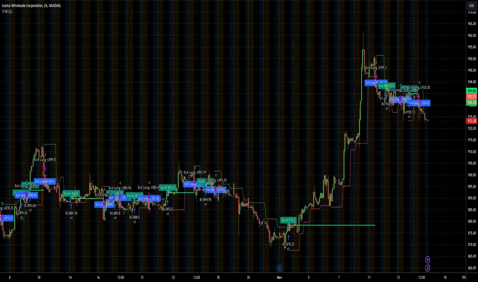
TFMTFM Strategy Explanation
Overview
The TFM (Timeframe Multiplier) strategy is a PineScript trading bot that utilizes multiple timeframes to identify entry and exit points.
Inputs
1. tfm (Timeframe Multiplier): Multiplies the chart's timeframe to create a higher timeframe for analysis.
2. lns (Long and Short): Enables or disables short positions.
Logic
Calculations
1. chartTf: Gets the chart's timeframe in seconds.
2. tfTimes: Calculates the higher timeframe by multiplying chartTf with tfm.
3. MintickerClose and MaxtickerClose: Retrieve the minimum and maximum closing prices from the higher timeframe using request.security.
- MintickerClose: Finds the lowest low when the higher timeframe's close is below its open.
- MaxtickerClose: Finds the highest high when the higher timeframe's close is above its open.
Entries and Exits
1. Long Entry: When the current close price crosses above MaxtickerClose.
2. Short Entry (if lns is true): When the current close price crosses below MintickerClose.
3. Exit Long: When the short condition is met (if lns is false) or when the trade is manually closed.
Strategy
1. Attach the script to a chart.
2. Adjust tfm and lns inputs.
3. Monitor entries and exits.
Example Use Cases
1. Intraday trading with tfm = 2-5.
2. Swing trading with tfm = 10-30.
Tips
1. Experiment with different tfm values.
2. Use lns to control short positions.
3. Combine with other indicators for confirmation.
NNFX RSI EMA FVMA MACD ALGOThis Pine Script introduces a cutting-edge trading strategy that seamlessly integrates multiple technical indicators—namely, the Flexible Variable Moving Average ( FVMA ), Relative Strength Index ( RSI ), Moving Average Convergence Divergence ( MACD ), and Exponential Moving Average ( EMA )—to deliver a sophisticated trading experience. This script stands out due to its comprehensive approach, robust risk management, and the inclusion of crucial data tables for various timeframes, making it an invaluable tool for traders seeking to enhance their market performance.
Originality of the Strategy:
The originality of this script lies in its unique combination of multiple powerful indicators, enabling traders to benefit from diverse perspectives on market dynamics. This mashup enhances decision-making processes, providing multiple layers of confirmation for trade entries and exits. The strategy is designed to offer an innovative solution for traders looking to improve their performance through well-defined rules and a solid framework.
Flexible Variable Moving Average (FVMA):
The FVMA adapts dynamically to market conditions, offering a more responsive trend line than traditional moving averages. This flexibility allows for quick identification of trends and reversals, crucial for fast-paced trading environments.
Exponential Moving Average (EMA):
By giving greater weight to recent price data, the EMA enhances sensitivity to price changes, allowing for more accurate entries and exits when used alongside the FVMA. This combination maximizes the effectiveness of the strategy in identifying optimal trading opportunities.
Relative Strength Index (RSI):
The RSI helps identify overbought or oversold conditions, integrating seamlessly with other indicators to enhance the strategy's ability to pinpoint potential reversal points. This aspect of the strategy ensures that traders can make informed decisions based on market momentum.
Moving Average Convergence Divergence (MACD):
The MACD serves as an essential confirmation tool, providing insights into trend strength and momentum. This enhances the accuracy of entry and exit signals, allowing traders to make more informed decisions based on robust technical analysis.
Multi-Take Profit (TP) and Stop Loss (SL) Levels:
The strategy supports multiple TPs, allowing traders to lock in profits at various levels while effectively managing risk through a robust SL system. This flexibility caters to diverse trading styles and risk profiles, ensuring that the strategy can adapt to individual trader needs.
Default Properties:
Take Profit Levels: TP1 is set to 2.0, and TP2 is set to 2.9, which is designed to enhance profit potential while maintaining a solid risk-reward ratio.
Stop Loss: A SL is set at 2% of the 5% account balance, which helps to preserve capital and manage risk effectively, adhering to the guideline of not risking more than 5-10% of the account balance per trade.
Labeling System for Exits: Automatic labeling of TP and SL exits on the chart provides clear visualization of trading outcomes. This feature supports informed decision-making and performance tracking, aligning with the guideline of providing transparent results.
Custom Alerts System:
The inclusion of customizable alerts for trade entries, exits, and SL/TP hits keeps traders informed in real-time, enabling prompt actions without constant market monitoring. This is crucial for effective trade management and helps traders respond quickly to market changes.
API Boxes for Automated Trading:
The strategy features API boxes, allowing traders to set up automated trading based on indicator signals. This functionality enables seamless integration with trading platforms, enhancing efficiency and streamlining the trading process, which is particularly valuable for traders looking to optimize their execution.
Data Tables for Enhanced Analysis:
The script includes data tables displaying critical insights across various timeframes: 2-hour, daily, weekly, and monthly. These tables provide a comprehensive overview of market conditions, allowing traders to analyze trends and make informed decisions based on a broad spectrum of data. By leveraging this information, traders can identify high-probability setups and align their strategies with prevailing market trends, significantly increasing their chances of success.
Default Properties:
Initial Capital: £1,000, ensuring a realistic starting point for traders.
Risk per Trade: 5% of the account balance, promoting sustainable trading practices.
Commission: 0.1%, reflecting realistic transaction costs that traders may encounter.
Slippage: 1%, accounting for potential market volatility during trade execution.
Take Profit Levels:
TP1: 2.0
TP2: 2.9
Stop Loss (SL): 2% of the 5% account balance, which is well within acceptable risk parameters.
Compliance with TradingView Guidelines:
This script fully complies with TradingView's guidelines, specifically:
Strategy Results:
The strategy is designed to publish backtesting results that do not mislead traders. The realistic parameters outlined in the default properties ensure that traders have a clear understanding of potential outcomes.
The dataset used for backtesting has sufficient trades to produce a reliable sample size, aligning with the guideline of ideally having more than 100 trades.
Any deviations from recommended practices are justified in the script description, ensuring transparency and adherence to best practices.
The script explains the default properties in detail, providing a thorough understanding of how these settings influence performance.
Why This Script is Worth Paying For:
This Pine Script offers an unparalleled trading experience through its unique combination of technical indicators, comprehensive trade management features, and detailed data tables for multiple timeframes. Here are compelling reasons to invest in this strategy:
Holistic Approach: The integration of multiple indicators ensures a well-rounded perspective on market conditions, increasing the likelihood of successful trades.
Advanced Risk Management: The flexibility of multiple TPs and SLs empowers traders to tailor their risk profiles according to individual strategies, enhancing overall profitability.
Automated Trading Capability: The inclusion of API boxes for automated trading streamlines execution, allowing traders to capitalize on opportunities without the need for manual intervention.
Comprehensive Data Analysis: The detailed data tables provide invaluable insights across different timeframes, enabling traders to make informed decisions based on robust market analysis.
In summary, this innovative Pine Script represents a powerful tool designed to empower traders at all levels. Its originality, synergistic functionality, and comprehensive features create a dynamic and effective trading environment, justifying its value and positioning it as a must-have for anyone serious about achieving consistent trading success.

Rsi Long-Term Strategy [15min]Hello, I would like to present to you The "RSI Long-Term Strategy" for 15min tf
The "RSI Long-Term Strategy " is designed for traders who prefer a combination of momentum and trend-following techniques. The strategy focuses on entering long positions during significant market corrections within an overall uptrend, confirmed by both RSI and volume. The use of long-term SMAs ensures that trades are made in line with the broader market trend. The stop-loss feature provides risk management by limiting losses on trades that do not perform as expected. This strategy is particularly well-suited for longer-term traders who monitor 15-minute charts but look for substantial trend reversals or continuations.
Indicators and Parameters:
Relative Strength Index (RSI):
- The RSI is calculated using a 10-period length. It measures the magnitude of recent price changes to evaluate overbought or oversold conditions. The script defines oversold conditions when the RSI is at or below 30 and overbought conditions when the RSI is at or above 70.
Volume Condition:
-The strategy incorporates a volume condition where the current volume must be greater than 2.5 times the 20-period moving average of volume. This is used to confirm the strength of the price movement.
Simple Moving Averages (SMA):
- The strategy uses two SMAs: SMA1 with a length of 250 periods and SMA2 with a length of 500 periods. These SMAs help identify long-term trends and generate signals based on their crossover.
Strategy Logic:
Entry Logic:
A long position is initiated when all the following conditions are met:
The RSI indicates an oversold condition (RSI ≤ 30).
SMA1 is above SMA2, indicating an uptrend.
The volume condition is satisfied, confirming the strength of the signal.
Exit Logic:
The strategy closes the long position when SMA1 crosses under SMA2, signaling a potential end of the uptrend (a "Death Cross").
Stop-Loss:
A stop-loss is set at 5% below the entry price to manage risk and limit potential losses.
Buy and sell signals are highlighted with circles below or above bars:
Green Circle : Buy signal when RSI is oversold, SMA1 > SMA2, and the volume condition is met.
Red Circle : Sell signal when RSI is overbought, SMA1 < SMA2, and the volume condition is met.
Black Cross: "Death Cross" when SMA1 crosses under SMA2, indicating a potential bearish signal.
to determine the level of stop loss and target point I used a piece of code by RafaelZioni, here is the script from which a piece of code was taken
I hope the strategy will be helpful, as always, best regards and safe trades
;)
Quatro SMA Strategy [4h]Hello, I would like to present to you The "Quatro SMA" strategy
Strategy is based on four simple moving averages of different lengths and monitoring trading volume. The key idea is to identify strong market trends by comparing short-term moving averages with the long-term SMA. The strategy generates buy signals when all short-term SMAs are above the SMA(200) and the volume confirms the strength of the move. Similarly, sell signals are generated when all short-term SMAs are below the SMA(200), and the volume is sufficiently high.
The strategy manages risk by applying a stop loss and three different Take Profit levels (TP1, TP2, TP3), with varying percentages of the position closed at each level.
Each Take Profit level is triggered at a specific percentage gain, with the position being closed gradually depending on the achieved targets. The percentage of the position closed at each TP level is also defined by the user.
Indicators and Parameters:
Simple Moving Averages (SMA):
The script utilizes four simple moving averages with different lengths (4, 16, 32, 200). The first three SMAs (SMA1, SMA2, SMA3) are used to determine the trend direction, while the fourth SMA (with a length of 200) serves as a support/resistance line.
Volume:
The script monitors trading volume and checks if the current volume exceeds 2.5 times the average volume of the last 40 candles. High volume is considered as confirmation of trend strength.
Entry Conditions:
- Long Position: Triggered when SMA1 > SMA2 > SMA3, the closing price is above SMA(200), and the volume condition is met.
- Short Position: Triggered when SMA1 < SMA2 < SMA3, the closing price is below SMA(200), and the volume condition is met.
Exit Conditions:
- Long Position: Closed when SMA1 < SMA2 < SMA3 and the closing price is above SMA(200).
- Short Position: Closed when SMA1 > SMA2 > SMA3 and the closing price is below SMA(200).
to determine the level of stop loss and target point I used a piece of code by RafaelZioni, here is the script from which a piece of code was taken
I hope the strategy will be helpful, as always, best regards and safe trades
;)
HilalimSB Strategy HilalimSB A Wedding Gift 🌙
What is HilalimSB🌙?
First of all, as mentioned in the title, HilalimSB is a wedding gift.
HilalimSB - Revealing the Secrets of the Trend
HilalimSB is a powerful indicator designed to help investors analyze market trends and optimize trading strategies. Designed to uncover the secrets at the heart of the trend, HilalimSB stands out with its unique features and impressive algorithm.
Hilalim Algorithm and Fixed ATR Value:
HilalimSB is equipped with a special algorithm called "Hilalim" to detect market trends. This algorithm can delve into the depths of price movements to determine the direction of the trend and provide users with the ability to predict future price movements. Additionally, HilalimSB uses its own fixed Average True Range (ATR) value. ATR is an indicator that measures price movement volatility and is often used to determine the strength of a trend. The fixed ATR value of HilalimSB has been tested over long periods and its reliability has been proven. This allows users to interpret the signals provided by the indicator more reliably.
ATR Calculation Steps
1.True Range Calculation:
+ The True Range (TR) is the greatest of the following three values:
1. Current high minus current low
2. Current high minus previous close (absolute value)
3. Current low minus previous close (absolute value)
2.Average True Range (ATR) Calculation:
-The initial ATR value is calculated as the average of the TR values over a specified period
(typically 14 periods).
-For subsequent periods, the ATR is calculated using the following formula:
ATRt=(ATRt−1×(n−1)+TRt)/n
Where:
+ ATRt is the ATR for the current period,
+ ATRt−1 is the ATR for the previous period,
+ TRt is the True Range for the current period,
+ n is the number of periods.
Pine Script to Calculate ATR with User-Defined Length and Multiplier
Here is the Pine Script code for calculating the ATR with user-defined X length and Y multiplier:
//@version=5
indicator("Custom ATR", overlay=false)
// User-defined inputs
X = input.int(14, minval=1, title="ATR Period (X)")
Y = input.float(1.0, title="ATR Multiplier (Y)")
// True Range calculation
TR1 = high - low
TR2 = math.abs(high - close )
TR3 = math.abs(low - close )
TR = math.max(TR1, math.max(TR2, TR3))
// ATR calculation
ATR = ta.rma(TR, X)
// Apply multiplier
customATR = ATR * Y
// Plot the ATR value
plot(customATR, title="Custom ATR", color=color.blue, linewidth=2)
This code can be added as a new Pine Script indicator in TradingView, allowing users to calculate and display the ATR on the chart according to their specified parameters.
HilalimSB's Distinction from Other ATR Indicators
HilalimSB emerges with its unique Average True Range (ATR) value, presenting itself to users. Equipped with a proprietary ATR algorithm, this indicator is released in a non-editable form for users. After meticulous testing across various instruments with predetermined period and multiplier values, it is made available for use.
ATR is acknowledged as a critical calculation tool in the financial sector. The ATR calculation process of HilalimSB is conducted as a result of various research efforts and concrete data-based computations. Therefore, the HilalimSB indicator is published with its proprietary ATR values, unavailable for modification.
The ATR period and multiplier values provided by HilalimSB constitute the fundamental logic of a trading strategy. This unique feature aids investors in making informed decisions.
Visual Aesthetics and Clear Charts:
HilalimSB provides a user-friendly interface with clear and impressive graphics. Trend changes are highlighted with vibrant colors and are visually easy to understand. You can choose colors based on eye comfort, allowing you to personalize your trading screen for a more enjoyable experience. While offering a flexible approach tailored to users' needs, HilalimSB also promises an aesthetic and professional experience.
Strong Signals and Buy/Sell Indicators:
After completing test operations, HilalimSB produces data at various time intervals. However, we would like to emphasize to users that based on our studies, it provides the best signals in 1-hour chart data. HilalimSB produces strong signals to identify trend reversals. Buy or sell points are clearly indicated, allowing users to develop and implement trading strategies based on these signals.
For example, let's imagine you wanted to open a position on BTC on 2023.11.02. You are aware that you need to calculate which of the buying or selling transactions would be more profitable. You need support from various indicators to open a position. Based on the analysis and calculations it has made from the data it contains, HilalimSB would have detected that the graph is more suitable for a selling position, and by producing a sell signal at the most ideal selling point at 08:00 on 2023.11.02 (UTC+3 Istanbul), it would have informed you of the direction the graph would follow, allowing you to benefit positively from a 2.56% decline.
Technology and Innovation:
HilalimSB aims to enhance the trading experience using the latest technology. With its innovative approach, it enables users to discover market opportunities and support their decisions. Thus, investors can make more informed and successful trades. Real-Time Data Analysis: HilalimSB analyzes market data in real-time and identifies updated trends instantly. This allows users to make more informed trading decisions by staying informed of the latest market developments. Continuous Update and Improvement: HilalimSB is constantly updated and improved. New features are added and existing ones are enhanced based on user feedback and market changes. Thus, HilalimSB always aims to provide the latest technology and the best user experience.
Social Order and Intrinsic Motivation:
Negative trends such as widespread illegal gambling and uncontrolled risk-taking can have adverse financial effects on society. The primary goal of HilalimSB is to counteract these negative trends by guiding and encouraging users with data-driven analysis and calculable investment systems. This allows investors to trade more consciously and safely.
What is HilalimSB Strategy🌙?
HilalimSB Strategy is a strategy that is supported by the HilalimSB algorithm created by the creator of HilalimSB and continues transactions with take profit and stop loss levels determined by users who strategically and automatically open transactions as a result of the data it receives and automatically closes transactions under necessary conditions. It is a first in the tradingview world with its unique take profit and stop loss markings. HilalimSB Strategy is open to users' initiatives and is a trading strategy developed on BTC.
What does the HilalimSB Strategy target?
The main purpose of HilalimSB Strategy is to reduce the transaction load of traders and to be integrated into various brokerage firms and operated by automatic trading bots, and it is aimed to serve this purpose. In addition to the strategies currently available in the markets, HilalimSB Strategy offers a useful infrastructure to traders with its useful interface. HilalimSB Strategy, which was decided to be published as a result of various calculations, was offered to the users with its unique visual effects after the completion of the testing procedures under market conditions.
HilalimSB Strategy and Heikin Ashi
HilalimSB Strategy produces data in Heikin Ashi chart types, but since Heikin Ashi chart types have their own calculation method, HilalimSB Strategy has been published in a way that cannot produce data in this chart type due to HilalimSB Strategy's ideology of appealing to all types of users, and any confusion that may arise is prevented in this way.
After the necessary conditions determined by the creator of HilalimSB are met, HilalimSB Heikin Ashi will be shared exclusively with invited users only, upon request, to users who request an invitation.
Differences between HilalimSB Strategy and HilalimSB
HilalimSB Strategy has been shared as a strategy and its features have been explained above. HilalimSB is a trading indicator and this is the main difference between them.We can explain it briefly this way.
Here are the differences between indicators and strategies:
1.Purpose and Use:
Indicators: Analyze market data to provide information about price movements and trends. They typically generate buy and sell signals and give traders clues about when to make trades in the market.
Strategies: These are plans for trading based on specific rules. They use signals from indicators and other market data to execute buy and sell transactions.
2.Features:
Indicators: Operate independently and are based on specific mathematical formulas. Examples include moving averages, RSI, and MACD.
Strategies: Combine one or more indicators and other market analysis tools to create a comprehensive trading plan. This plan determines entry and exit points, risk management, and trade size.
3.Scope:
Indicators: Are single analysis tools focusing on specific time frames or price movements.
Strategies: Are comprehensive trading plans that typically involve multiple trades over a certain period.
4.Decision Making:
Indicators: Provide information to traders and help in the decision-making process.
Strategies: Are direct decision-making mechanisms that execute trades automatically according to predetermined rules.
5.Automation:
Indicators: Are mostly interpreted manually and used based on the trader’s discretion.
Strategies: Can be used in automated trading systems and execute trades automatically according to the set rules.
The shared image is a 1-hour chart of BTCUSDC.P determined by the user as 1 percent take profit and 1 percent stop loss. And transactions were opened on Binance with the commission rate determined as 0.017 for the USDC trading pair.
HilalimSB Strategy, which presents users with completely concrete data, has proven itself in testing processes and is a project of SB that aims to reach all user profiles.🌙

[Support and Resistance with Trend Lines] with Backtest (TSO) with Backtest (TSO)
===========================================================================
===========================================================================
This indicator serves as a comprehensive full-cycle trading system, providing alerts at each stage of the trade, from opening to closure. The algorithm uses most recent and historical S&R (Support and Resistance) levels with most recent and historical Trend Lines, generating signals for trades when Breaks/Bounces occur (Trade Open Signal triggers can be configured via very customizable indicator Input "Signal Trigger Matrix" settings). With signal for trade open, TP (Take Profit and SL (Stop Loss) levels are calculated as well and marked on the chart including alerts for each action of the trade. The indicator offers a variety of automated approaches for TP (Take-Profit) and SL (Stop-Loss) settings. These include static current/historical S&R (Support and Resistance) levels or S&R/Trend Lines dynamic breaks for TP (Take-Profit) and various SL (Stop-Loss) approaches, including ATR Trailing SL, opposite S&R (Support and Resistance) levels SL, opposite Trend Lines SL and more. This diverse set of tools ensure flexibility in tailoring TP (Take-Profit) and SL (Stop-Loss) parameters to different market conditions, contributing to a more adaptive and robust trading system. Additionally, a series of signal analysis tools, including market sentiment, candle bar analysis, divergence, and volume, enhance the precision of trading signals.
* Works with popular timeframes: 1M, 3M, 5M, 15M, 30M, 45M, 1H.
* Works well with Futures and Indices, can be used to trade Stocks, Crypto and FOREX.
* Includes LIVE alert/labels Breakouts and Bounces signal trigger feature, which can be used for scalping (NOTE: This approach cannot be backtested).
* Every action of the trade is calculated on a confirmed closed candle bar state (barstate.isconfirmed), so the indicator will never repaint.
==============================================================
Indicator examples:
---------------------------------------------------------------------------
Strategy Config: SRTL_MES_15M3Y_EODoff_ALL
Here is a nice example of MES (Micro E-Mini S&P 500 Index Futures) configuration, which uses S&R (Support and Resistance) breakouts as signal trigger with Elliot Wave confirmation and previous S&R historical levels for TP (Take-Profit).
---------------------------------------------------------------------------
An example of an intraday Tesla trade. Also the green arrows will be displayed IMMEDIATELY when Breakout/Reverse Bounce occurs (same an Alert will be triggered immediately).
===========================================================================
Trading open/close/TP/SL labels, plots and colors explanations:
---------------------------------------------------------------------------
>>> S&R (Support and Resistance) levels/lines: orange - support, blue - resistance (can be hidden).
>>> Trend Lines: yellow - support, green - resistance (can be hidden).
>>> Blue labels show resistance breakouts and bounces, light-blue - bullish, dark-blue - bearish
>>> Yellow labels show resistance breakouts and bounces, light-yellow - bullish, dark-yellow - bearish
>>> Green/Red arrows on top/bottom of candle bar will show LIVE breakouts (if turned on)
>>>>> LONG open: green "house" looking arrow below candle bar.
>>>>> SHORT open: red "house" looking arrow above candle bar.
>>>>> LONG/SHORT take-profit target: green/red circles (multi-profit > TP2/3/4/5 smaller circles).
>>>>> LONG/SHORT stop-loss target: green/red + crosses.
>>>>> LONG/SHORT take-profit hits: green/red diamonds.
>>>>> LONG/SHORT stop-loss hits: green/red X-crosses.
>>>>> LONG/SHORT EOD (End of Day | Intraday style) close (profitable trade): green/red squares.
>>>>> LONG/SHORT EOD (End of Day | Intraday style) close (loss trade): green/red PLUS(+)-crosses.
===========================================================================
STATS TABLE ///////////////////////////////////////////////////////////////
---------------------------------------------------------------------------
>>> Trading STATS table on the chart showing current trade direction, Last TP (Take-Profit) Taken, Current Trade PL (profit/loss in price difference from trade open to the very current state).
---------------------------------------------------------------------------
CUSTOM TRADING DATE RANGE /////////////////////////////////////////////////
---------------------------------------------------------------------------
>>>>> This feature can be used to manually set indicator trading range from and to a specific date and time. NOTE: This is not intended for a very long date range backtesting, utilize TradingView Strategy Tester for that.
* Use TradingView “Strategy Tester” to see Backtesting results
NOTE: If Strategy Tester does not show any results with Date Ranged fully unchecked, there may be an issue where a script opens a trade, but there is not enough TradingView power to set the Take-Profit and Stop-Loss and somehow an open trade gets stuck and never closes, so there are “no trades present”. In such case - manually check “Start”/“End” dates or use “Deep Backtesting” feature!
---------------------------------------------------------------------------
INTRADAY ACTIVE TRADING SESSION CONFIGURATION /////////////////////////////
---------------------------------------------------------------------------
>>> Regional Active Trading Session Hours Schedule: If selected - trades will only open during regional active trading session, if 'OFF', there will be no trading schedule and trades will open 24/7.
>>> EOD(End of Day) Close - On/Off: Close the trade if it's still open at the end of active trading session (on the very last candle bar). NOTE: If no region is selected at 'Regional Active Trading Session Schedule' - there will be no EOD(End of Day) Close and trades will run overnight until either SL(Stop-Loss) or TP(Take-Profit) is hit!
>>>>> EOD(End of Day) Close - 1 candle bar before last: This is specifically for stocks as while usually indices can be closed 15minutes after the market closes, for stocks - the last candle bar closes at the same time with the market active trading session, which if closed - trades can't be closed until next day/session! Enable this setting for the trade to close/alert 1 candle bar before the last one, so there is still time to close the trade at the Broker (NOTE: depending on the timeframe, 1 candle bar can be: 15sec, 30sec, 1min, 3min, 5min, 15min, 30min, 45min, 1h).
---------------------------------------------------------------------------
SIGNAL TRIGGER MATRIX ////////////////////////////////////////////////
---------------------------------------------------------------------------
>>> Trading Engine: This setting turns on TradingView Strategy trading engine for backtesting.
>>> Market Session Only: With this setting turned on, all signal trigger Breaks/Bounces will be hidden during Pre/Post market time.
>>> Plot S&R Levels/Lines: Plot S&R (Support and Resistance) on chart. Note: historical levels/lines will only be plotted if hit (Break/Bounce).
>>> Plot Trend Lines Levels/Lines: Plot Trend Lines levels/lines on chart. Note: historical levels/lines will only be plotted if hit (Break/Bounce).
>>> Use S&R Current Levels | Use S&R Historical Levels | Use Trend Lines Current Levels | Use Trend Lines Historical Levels |: Choose which levels should be used for Breaks/Bounces to be captured on. If all triggers are turned on/checked - whatever happens 1st wins the trigger.
>>> Breaks | Bounces: 'Breaks': Turn on Breaks through levels/lines signal trigger. | 'Bounces': Turn on Bounces off levels/lines signal trigger.
>>> Signal: Regular | Signal: S&R Combo | Signal: TL Combo | Signal: S&R + TL Combo | Signal: Repeat Action |: Trade open signal trigger execution approach MATRIX (If 1 or more turned on at the same time - whatever comes first will be the trade signal trigger). 'Regular': A single Break/Bounce must occur on a closed bar for signal trigger. 'S&R Combo': A combination of 2 Current + Historical S&R (Support and Resistance) Break/Bounce must happen in the same direction on same bar for signal trigger. 'TL Combo': A combination of 2 Current + Historical Trend Lines Break/Bounce must happen in the same direction on same bar for signal trigger. 'S&R + TL Combo': a combination of ANY S&R and Trend Line Break/Bounce must happen in the same direction on same bar for signal trigger. 'Repeat Action': Initial and then confirmation (2nd/3rd/etc. consecutive occurence) Break/Bounce must occur on same level/line for signal trigger.
>>> Historical - Look Back (# of days): How far back (in # of days) will historical S&R/Trend Lines will be used for Trade Open signals/TP/SL/etc.
>>> Historical - Look Back Invalidation (# of days): IF THERE IS TOO MUCH HISTORICAL LEVELS/LINES ON CHART - LOWER THIS SETTING + MAKE SURE IT'S SMALLER THAN 'Historical - Look Back (# of days)'. With big Look back period (5+ days) - it can become very messy with too many historical levels/lines. To clear oldest historical levels/lines - set Look Back Invalidation # of days to less than Historical Look Back # of days. (After X # of Look Back Invalidation days - older levels/lines will become invalidated and no longer used for opening trades/TP (Take-Profit)/SL (Stop-Loss), while newer levels/lines will still be discovered.
>>> S&R/Trend Lines - Support/Resistance combined into 1 entity: Every level or a line becomes simply a level or a line, regardless if it originally was a support or resistance. By default, depending on the level/line originally being support or resistance - the signal direction will be such as: Resistance is broken > LONG / bounced > SHORT; Support is broken > SHORT / bounced > LONG; with this setting on, either level or line can be both broken or bounced off in ANY direction, trade open direction will depend on current market sentiment only.
---------------------------------------------------------------------------
S&R CONFIGURATION ////////////////////////////////////////////////
---------------------------------------------------------------------------
>>> S&R Search - Left Bars (current): This setting is for calculating optimal S&R (Support and Resistance) levels (in combination with below - Right Bars).
>>> S&R Search - Right Bars (current): This setting is for calculating optimal S&R (Support and Resistance) levels (in combination with above - Left Bars).
>>> S&R Search - Custom Resolution (current): This is a custom timeframe setting specifically for S&R Search, it disregards current chart timeframe. This is great to use for scalping, for example: with main chart set to 1min and the custom timeframe set to 3min or 5min - there will be stronger support/resistance levels with more detailed price action.
>>> S&R Search - Left Bars (historical): This setting is for calculating optimal S&R (Support and Resistance) levels (in combination with below - Right Bars).
>>> S&R Search - Right Bars (historical): This setting is for calculating optimal S&R (Support and Resistance) levels (in combination with above - Left Bars).
>>> S&R Search - Custom Resolution (historical): This is a custom timeframe setting specifically for S&R Search, it disregards current chart timeframe. This is great to use for scalping, for example: with main chart set to 1min and the custom timeframe set to 3min or 5min - there will be stronger support/resistance levels with more detailed price action.
>>> S&R - Historical S&R Levels - Extend to the right: Extend all S&R lines to the right.
>>> S&R (Current/Historical) - Live Breakout/Bounce - ALERT/SHOW: NOTE: Alert wlil trigger immediately at price Breaking thru or Bouncing off level/line and an arrow above /below the bar will show the direction of breakout/bounce. If on that same live bar - price comes back causing the Breakout/Bounce become no longer valid - the arrow will disappear as the condition of the Break/Bounce will no longer be valid.
---------------------------------------------------------------------------
TREND LINES CONFIGURATION ////////////////////////////////////////////////
---------------------------------------------------------------------------
>>> Show: Trend Line development (where it 'did not exist' yet): It takes 2 pivots to develop a trend line, pivot is established at least 3 candle bars later from where the pivot is. With this setting turned on - it will plot dashed lines where trend lines originated connecting the 1st and 2nd pivot point up to where the trend line became established (where in reality you would now be able to draw a certain trend line). Established already generated trend line are plotted with a solid line.
>>> Trend Lines - Line Slope Confirmation: LONG breakout will only be shown if trend line is goind downslope \. SHORT breakout will only be shown if trend line is goind upslope /.
>>> Trend Lines - Search - Left Bars (current): This setting is for calculating optimal Trend Lines.
>>> Trend Lines - Search - Right Bars (current): This setting is for calculating optimal Trend Lines.
>>> Trend Lines - Custom Resolution (current): This is a custom timeframe setting specifically for S&R Search, it disregards current chart timeframe. This is great to use for scalping, for example: with main chart set to 1min and the custom timeframe set to 3min or 5min - there will be stronger support/resistance levels with more detailed price action.
>>> Trend Lines - Search - Left Bars (historical): This setting is for calculating optimal Trend Lines.
>>> Trend Lines - Search - Right Bars (historical): This setting is for calculating optimal Trend Lines.
>>> Trend Lines - Custom Resolution (historical): This is a custom timeframe setting specifically for S&R Search, it disregards current chart timeframe. This is great to use for scalping, for example: with main chart set to 1min and the custom timeframe set to 3min or 5min - there will be stronger support/resistance levels with more detailed price action.
>>> Trend Lines - Historical Trend Lines - Extend to the right: Extend all Trend Lines to the right.
>>> Trend Lines (Current/Historical) - Live Breakout/Bounce - ALERT/SHOW: NOTE: Alert will trigger immediately at price Breaking thru or Bouncing off level/line and an arrow above /below the bar will show the direction of breakout/bounce. If on that same live bar - price comes back causing the Breakout/Bounce become no longer valid - the arrow will disappear as the condition of the Break/Bounce will no longer be valid.
---------------------------------------------------------------------------
TAKE-PROFIT/STOP-LOSS CONFIGURATION ///////////////////////////////////////
---------------------------------------------------------------------------
>>> TP (Take-Profit) System: 'S&R Static Current/Historical': TP (Take-Profit) is calculated using current/historical S&R (Support & Resistance) levels at trade open and remains static. 'S&R/Trend Lines Dynamic Breaks': TP (Take-Profit) is fully dynamic and will be trigger at price above trade open price and with Breakout occurence (S&R or Trend Line current/historical breakout).
>>> TP (Take-Profit) # of targets: It is wise to divide the trade into several profit targets. With this setting - up to 5 TP (Take-Profit) targets can be approached. The trade will be equally divided up by the selected # of TP (Take-Profit) targets.
>>> SL (Stop-Loss) System: 'ATR-Trailing-SL': SL (Stop-Loss) is trail-following the ATR (Average True Range) line, NOTE: If at signal trigger, ATR will be against the trade direction - trade open signal will be skipped; 'S&R-Static-SL': SL (Stop-Loss) is set at trade open per optimal most recent S&R level and remains there until trade closes; 'TrendLines-Static-SL': SL (Stop-Loss) is set at trade open per optimal most recent trend line and remains there until trade closes; 'TrendLines-Dynamic-SL': SL (Stop-Loss) will be set per current opposite trend line and follow it until trade is open.; 'Oppos-Sig-Trd-in-Loss': SL (Stop-Loss) will trigger at opposite signal with trade currently at loss.
>>> SL (Stop-Loss) - On/Off: Without SL (Stop-Loss), unless EOD (End of Day) Close is turned on - there will be no SL (Stop-Loss) at all!
---------------------------------------------------------------------------
MARKET SENTIMENT CONFIRMATION ///////////////////////////////////////
---------------------------------------------------------------------------
>>> Market Sentiment: Signal is confirmed per Market Sentiment direction. If Market Sentiment is turned off - whatever signal comes 1st will be the trade open trigger.
---------------------------------------------------------------------------
SIGNAL ANALYSIS AND CLEANUP ///////////////////////////////////////////////
---------------------------------------------------------------------------
>>> Signal Cleanup - Bar Color: Include Bar Color (bullish/bearish) confirmation, LONG signal will only be opened if signal bar is green/bullish, SHORT if red/bearish.
>>> Signal Cleanup - Bar Directional Structure: Skip opposite bar structure types signals (For example: bearish green hammer).
>>> Signal Cleanup - Bar Doji Skip: Skip doji (indecisive) candles signals.
>>> Signal Cleanup - EWO (Elliott Wave Oscillator): Include EWO (Elliott Wave Oscillator), LONG will only be opened if EWO is bullish / SHORT if EWO is bearish.
>>> Signal Cleanup - VWAP (Volume-Weighted Average Price): Include VWAP (Volume-Weighted Average Price), LONG will only be opened if price is above VWAP / SHORT if price is below VWAP.
>>> Signal Cleanup - MA (Moving Average) Confirmation: Include MA (Moving Average), LONG will only be opened if MA is bullish / SHORT if MA is bearish.
>>> Signal Cleanup - ATR (Average True Range): Include ATR (Average True Range) confirmation, LONG will only be opened if ATR is bullish / SHORT if ATR is bearish.
>>> Signal Cleanup - Divergence(RSI + MACD): Include Divergence (RSI + MACD ) confirmation, LONG will only be opened if Divergence is bullish / SHORT if Divergence is bearish.
>>> Signal Cleanup - Volume % Strength: Include Volume strength/percentage confirmation, LONG/SHORT will only be opened with strong Volume matching the signal direction | By default, strong Volume percentage is set to 150% and weak to 50%.
>>> Signal Cleanup - Volume Above Average: Include Volume Above Moving Average (Volume closing bar closes above volume moving average) confirmation, LONG/SHORT will only be opened with Volume above average - Volume closed bar color must match the closed price color (bullish/bearish direction) + Volume bar must be closed above volume MA line).
---------------------------------------------------------------------------
===========================================================================
||||||||||||||||||||||||||||||||||| *** ||||||||||||||||||||||||||||||||||| *** |||||||||||||||||||||||||||||||||||
||||||||||||||||||||||||||||||||||| *** ||||||||||||||||||||||||||||||||||| *** |||||||||||||||||||||||||||||||||||
TP System - VERY IMPORTANT INFO!
-------------------------------------------------------------------------------------------------------------------
"TP PERCENTAGE" - amount by which current trade/position needs to be reduced/partially closed/sold.
-------------------------------------------------------------------------------------------------------------------
TP System: Dynamic
"TP PERCENTAGE" - will always be the same amount (trade/position size divided by the # of take-profit(TP) targets) and percentage to be closed will always be of the ORIGINAL trade/position.
-------------------------------------------------------------------------------------------------------------------
TP System: Static
"TP PERCENTAGE" - will always be the same amount IF take-profit(TP) targets are hit 1-by-1 (TP1 > TP2 > TP3 > TP4 > TP5), otherwise it will vary and unless it is a 1st take-profit(TP1), the REMAINING trade/position size will always be smaller than original and therefore the percentage to be closed will always be of the REMAINING trade/position and NOT the original one!
-------------------------------------------------------------------------------------------------------------------
"TP PERCENTAGE" CheatSheet (these are the only percentages you may see)
-----------------------------------------------------------------------
TP PERCENTAGE---Close/Sell Amount-------------Example (trade size: 50 stocks)
20%-------------trade size * 0.2--------------50 * 0.2 = 10 stocks
25%-------------trade size * 0.25-------------50 * 0.25 = 12.5(~13) stocks
34%-------------trade size * 0.34-------------50 * 0.34 = 17 stocks
40%-------------trade size * 0.4--------------50 * 0.4 = 20 stocks
50%-------------trade size * 0.5--------------50 * 0.5 = 25 stocks
60%-------------trade size * 0.6--------------50 * 0.6 = 30 stocks
66%-------------trade size * 0.66-------------50 * 0.66 = 33 stocks
75%-------------trade size * 0.75-------------50 * 0.75 = 37.5(~38) stocks
80%-------------trade size * 0.8--------------50 * 0.8 = 40 stocks
100%------------trade size--------------------50 = 50 stocks
-----------------------------------------------------------------------
If for any reason a portion of the current/remaining trade closed at such occurrence was slightly wrong, it is not an issue. Such occurrences are rare and with slight difference in partial TP closed is not significant to overall performance of our algorithms.
||||||||||||||||||||||||||||||||||| *** ||||||||||||||||||||||||||||||||||| *** |||||||||||||||||||||||||||||||||||
||||||||||||||||||||||||||||||||||| *** ||||||||||||||||||||||||||||||||||| *** |||||||||||||||||||||||||||||||||||
===========================================================================
Alert Settings (you don’t have to touch this section unless you will be using TradingView alerts through a Webhook to use with trading bot)
---------------------------------------------------------------------------
Here is how a LONG OPEN alert looks like.
NOTE: Each label , , etc. is customizable, you can change the text of it within indicator Input settings.
ALERT >>>>>>>>>>>>>>>>>>>>>>>>>>>>>>>>>>>>>>>>>>>>>>>
COIN: BTCUSD
TIMEFRAME: 15M
LONG: OPEN
ENTRY: 20000
TP1: 20500
TP2: 21000
TP3: 21500
TP4: 22500
TP5: 23500
SL: 19000
Leverage: 0
---------------------------------------------------------------------------
Here is how a TP1 alert will look with 5 TPs breakdown of the trade.
NOTE1: Next to TP1 taken it will show at which price it was triggered.
NOTE2: Next to "TP Percentage" it shows how much of the CURRENT/ACTIVE/REMAINING trade needs to be closed.
NOTE2: If TP2/3/4/5 comes before TP1 - the alert will tell you exactly how many percent of the trade needs to be closed!
ALERT >>>>>>>>>>>>>>>>>>>>>>>>>>>>>>>>>>>>>>>>>>>>>>>
COIN: BTCUSD
TIMEFRAME: 15M
LONG: TP1
TP1: 20500
TP Percentage: 20%
---------------------------------------------------------------------------
Here is how an alert will look for LONG - STOP-LOSS.
ALERT >>>>>>>>>>>>>>>>>>>>>>>>>>>>>>>>>>>>>>>>>>>>>>>
COIN: BTCUSD
TIMEFRAME: 15M
ENTRY: 20000
LONG: SL
SL: 19000
---------------------------------------------------------------------------
Here is how an alert will look for LONG - EOD (End of Day) In Profit close.
ALERT >>>>>>>>>>>>>>>>>>>>>>>>>>>>>>>>>>>>>>>>>>>>>>>
COIN: BTCUSD
TIMEFRAME: 15M
LONG: EOD-Close (profit)
ENTRY: 20000
EOD-Close: 21900
===========================================================================
Adding Alerts in TradngView
---------------------------------------------------------------------------
-Add indicator to chart and make sure the correct strategy is configured (check Backtesting results)
-Right-click anywhere on the TradingView chart
-Click on Add alert
-Condition: Select this indicator by it’s name
-Immediately below, change it to "alert() function calls only", as other wise there will be 2 alerts for every alert!
-Expiration: Open-ended (that may require higher tier TradingView account, otherwise the alert will need to be occasionally re-triggered)
-Alert name: Whatever you desire
-Hit “Create”
-Note: If you change ANY Settings within the indicator – you must DELETE the current alert and create a new one per steps above, otherwise it will continue triggering alerts per old Settings!
===========================================================================
Good Luck! (NOTE: Trading is very risky, past performance is not necessarily indicative of future results, so please trade responsibly!)
---------------------------------------------------------------------------
NOTE: There seems to be a strange glitch when strategy is running live, it will show "double-take" take-profits labels on the chart. This is not affecting the script logic and backtesting results, if you simply change the timeframe real quick to something else then back - it will no longer show the duplicate orders... this must be some sort of a glitch as every alert was thoroughly tested to make sure everything is working!
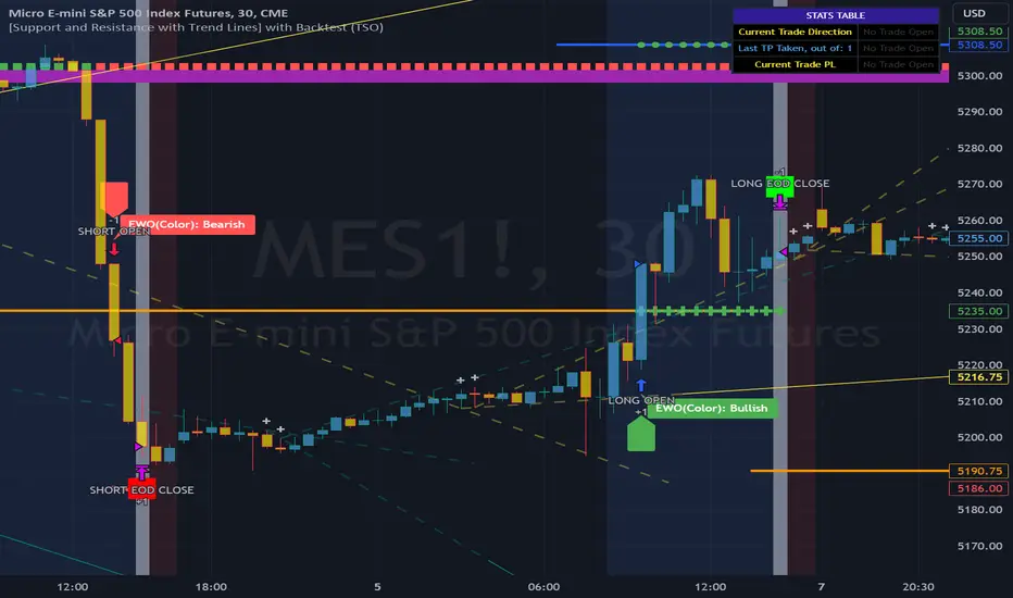
Spot Martingale KuCoin - The Quant ScienceINTRODUCTION
Backtesting software of the Spot Martingale algorithm offered by the KuCoin exchange.
This script replicates the logic used by the KuCoin bot and is useful for analyzing strategy on any cryptocurrency historical series.
It's not intended as an automatic trading algorithm and does not offer the possibility of automatic order execution.
The trader will use this software exclusively to research the best parameters with which to work on KuCoin.
LOGIC OF EXECUTION
The execution of orders is composed as follows:
1) Start Martingale: initial order
2) Martingale-Number: orders following Start Martingale
(A) The software is designed and developed to replicate trading without taking into account technical indicators or particular market conditions. The Initial Order (Start Martingale) will be executed immediately the close of the previous Martingale when the balance of market orders is zero. It will use the capital set in the Properties section for the initial order.
(B) After the first order, the software will open new orders as the price decreases. For orders following Start Martingale, the initial capital, multiplier, and number of orders in the exponential growth context are considered. The multiplier is the factor that determines the proportional increase in capital with each new order. The number of orders, indicates how many times the multiplier is applied to increase the investment.
Example
To find out the capital used in Martingale order number 5, with a Multiple For Position Increase equal to 2 and a starting capital of $100, the formula will be as follows:
Martingale Order = ($100 * (2 * 2 * 2 * 2 * 2)) = $100 * 32 = $3.200
(C) A multiplier is used for each new order that will increase the quantity purchased.
(D) All previously open orders are closed once the take profit is reached.
USER MANUAL
The user interface consists of two main sections:
1. Settings
Percentage Drop for Position Increase (0.1-15%) : percentage distance between Martingale orders. For example, if you set 5% each new order will be opened after a 5% price decrease from the previous one.
Max Position Increases (1-15) : number of Martingale orders to be executed after Start Martingale. For example, if you set 10, up to10 orders will be opened after Start Martingale.
Multiple For Position Increase (1-2x) : capital multiplier. For example, if you set 2 each for each new order, the capital involved will be doubled, order by order.
Take Profit Percentage (0.5-1000%) : percentage take profit, calculated on the average entry price.
2. Date Range Backtesting
The Date Range Backtesting section adjusts the analysis period. The user can easily adjust the UI parameters, and automatically the software will update the data.
LIMITATIONS OF THE MODEL
Although the Martingale model is widely used in position management, even this model has limitations and is subject to real risks during particular market conditions. Knowing these conditions will help you understand which asset is best to use the strategy on.
The main risks in adopting this automatic strategy are 2:
1) The price falls below our last order.
It happens during periods of strong bear-market in which the price collapses abruptly without experiencing any pullback. In this case the algorithm will enter a drawdown phase and the strategy will become a loser. The trader will then have to consider whether to wait for a price recovery or to incur a loss by manually closing the algorithm.
2) The price increases quickly.
It happens during periods of strong bull-market in which the price rises abruptly without experiencing any pullback. In this case the algorithm will not optimize order execution, working only with Start Martingale in the vast majority of trades. Given the exponential nature of the investment, the algorithm will in this case generate a profit that is always less than that of the reference market.
The best market conditions to use this strategy are characterized by high volatility such as correction phases during a bull run and/or markets that exhibit sideways price trends (such as areas of accumulation or congestion where price will generate many false signals).
FEATURES
This script was developed by including features to optimize the user experience.
Includes a dashboard at launch that allows the user to intuitively enter backtesting parameters.
Includes graphical indicator that helps the user analyze the behavior of the strategy.
Includes a date period backtesting feature that allows the user to adjust and choose custom historical periods.
DISCLAIMER
This script was released using parameters researched solely for the BTC/USDT pair, 4H timeframe, traded on the KuCoin Exchange (2017-present). Do not consider this combination of parameters as universal and usable on all assets and timeframes.
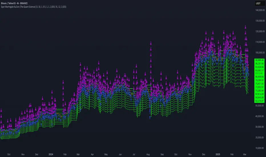
BitBell - EMA PullBack RSI EXO
🔵 Introduction
Version 1.1
This is a Pine 5 trend following strategy. It has a four strategy with several alerts and signals. The design intent is to produce a commercial grade signal generator that can be adapted to any symbol in cryptocurrency and only 1H Chart. Ideally, the script is reliable enough to be the basis of an automated trading system web-hooked to a server with API access to crypto brokerages. The strategy can be run in three different modes: long, short and bidirectional.
As a trend following strategy, the behavior of the script is to buy on strength and sell on weakness. As such the trade orders maintain its directional bias according to price pressure. What you will see on the chart is long positions on the left side of the mountain and short on the right. Long and short positions are not intermingled as long as there exists a detectable trend. This is extremely beneficial feature in long running bull or bear markets. The script uses multiple setups to avoid the situation where you got in on the trend, took a small profit but couldn’t get back in because the logic is waiting for a pullback or some other intricate condition.
Deep draw-downs are a characteristic of trend following systems and this system is no different. However, this script makes use of the TradingView pyramid feature with three NPUs to find better place and even you can change drop percentage in settings for another trigger, accessible from the properties tab.
When trend market break it will stop the trade and usually it takes 2-4 percent loss but don't worry it has prefect money management and you can use it for Futures market and even Spot market.
🔵 Design
This script uses twelve indicators on two time frames. The chart (primary) interval and one higher time frame which is based on the primary. The higher time frame identifies the trend for which the primary will trade. I’ve tried to keep the higher time frame around five times greater than the primary. The original trading algorithms are a port from a much larger program on another trading platform. I’ve converted some of the statistical functions to use standard indicators available on TradingView. The setups make heavy use of the Hull Moving Average in conjunction with EMAs that form the Bill Williams Alligator as described in his book “New Trading Dimensions” Chapter 3. Lag between the Hull and the EMAs form the basis of the entry and exit points. The alligator itself is used to identify the trend main body.
The entire script is around 740 lines of Pine code which is the maximum incidental size given the TradingView limits: local scopes, run-time duration and compile time. I’ve been working on this script for over a year and have tested it on various instruments stock crypto. It performs well on higher liquidity markets that have at least a year of historical data. Though it can be configured to work on any interval between 15 minutes and 4 hour, trend trading is generally a longer term paradigm. For day trading the 10 to 15 minute interval will allow you to catch momentum breakouts. For intraweek trades 30 minutes to 1 hour should give you a trade every other a day.
Inputs to the script use cone centric measurements in effort to avoid exposing adjustments to the various internal indicators. The goal was to keep the inputs relevant to the actual trade entry and exit locations as opposed to a series of MA input values and the like. As a result the strategy exposes over 12 inputs grouped into long or short sections. Inputs are available for the usual minimum profit and stop-loss as well as trade, modes, presets, reports and lots of calibrations. The inputs are numerous, I’m aware. Unfortunately, at this time, TradingView does not offer any other method to get data in the script. The usual initialization files such as cnf, cfg, ini, json and xml files are currently unsupported.
Example configurations for various instruments along with a detailed PDF user manual is available.
it has no repaint i guaranty this, and you can have 10 days free with comment and check it by yourself
One issue that comes up when comparing the strategy with the study is that the strategy trades show on the chart one bar later than the study. This problem is due to the fact that “strategy.entry()” and “strategy_close()” do not execute on the same bar called. The study, on the other hand, has no such limitation since there are no position routines. However, alerts that are subsequently fired off when triggered in the study are dispatched from the TradingView servers one bar later from the study plot. Therefore the alert you actually receive on your cell phone matches the strategy plot but is one bar later than the study plot.
Please be aware that the data source matters. Cryptocurrency has no central tick repository so each exchange supplies TradingView its feed. Even though it is the same symbol the quality of the data and subsequently the bars that are supplied to the chart varies with the exchange. This script will absolutely produce different results on different data feeds of the same symbol. Be sure to backtest this script on the same data you intend to receive alerts for. Any example settings I share with you will always have the exchange name used to generate the test results.
🟡 Usage
It sends long and short signals with pyramid orders of up to 3, meaning that the strategy can trigger up to 3 orders in the same direction. Good risk and money management.
It's important to note that the strategy combines 2 systems working together (Long and LongX). Let’s describe the specific features of this strategy.
🔵 If Findes Supports And Ressitances And Trend Lines As Best As It Can, And You Can See:
🟢 Frist Simple Long Condition = It Look At The Trend Wait For RSI Cross 30 Number Then Ckeck Risk To Reward, check something else such as divergence:
🟢 Another Long Example:
🔴 Frist Simple Short Condition = It Look At The Trend Wait For RSI Cross 70 Number Then Ckeck Risk To Reward, check something else such as divergence:
🔴 Another Short Example:
The following steps provide a very brief set of instructions that will get you started but will most certainly not produce the best backtest. A trading system that you are willing to risk your hard earned capital will require a well crafted configuration that involves time, expertise and clearly defined goals. As previously mentioned, I have several example configs that I use for my own trading that I can share with you along with a PDF which describes each input in detail. To get hands on experience in setting up your own symbol from scratch please follow the steps below.
The input dialog box contains over 12 inputs, There are four options must to be configured: Choose Target, side, Choose Settings, Money Management,and settings that apply to both. The following steps address these four main options only.
Money Management System For Leverage 10:
Bot Finds Last Lower Low And Calculate Distance From Entry Price, Then Cross It To Initial Capitan And Cross Leverage =>
Position_Size = (((1.64) * (initial Capital)) * (leverage))
And Check Dominances Too For Getting Best Money Management Result
🔵 Settings
* Side, You Can Set Long Or Short Or Both.
* Choose Target, You Can Set One Target Or All Targets.
* Money Management, You Can ON Or OFF It, With OFF You Can USE It For SPOT Trades.
* Choose Settings, In This Field You Can Set Mathematical Optimization, Ddepends On Which Pair You USE.
* Clear With Daily PullBack?, With This Check Box You Can Clear Signals With Daily PullBack.
* Long X, You Can Set Long Leverage.
* Short X, You Can Set Short Leverage.
* Second Order X, You Can Set Pyramiding Leverage.
* Target Long, You Can Set Percent For Long Target.
* Target Short, You Can Set Percent For Short Target.
* Short Martin Percent, You Can Set Short Martingale Percent.
* Long Martin Percent, You Can Set Long Martingale Percent.
🟡 Pyraming 3
🟡 Commission Is 0.065 %
🟡 Slippage Is 10 ticks
🔴Only Use For 1 Hour Chart
🔴 CONCLUSION
We believe that success lies in the association of the user with the indicator, opposed to many traders who have the perspective that the indicator itself can make them become profitable. The reality is much more complicated than that.
The aim is to provide an indicator comprehensive, customizable, and intuitive enough that any trader can be led to understand this truth and develop an actionable perspective of technical indicators as support tools for decision making.
🔴 RISK DISCLAIMER
Trading is risky & most day traders lose money. All content, tools, scripts, articles, & education provided by BitBell are purely for informational & educational purposes only. Past performance does not guarantee future results.

[Opening Range Breakout] S&R Strategy with Backtest (TSO) S&R Strategy with Backtest (TSO)
===========================================================================
===========================================================================
This indicator serves as a comprehensive full-cycle trading system, providing alerts at each stage of the trade, from opening to closure. The algorithm initiates by calculating the Opening/Pre-Market Price Range, waiting for a breakout to generate signals, and establishing TP (Take Profit and SL (Stop Loss) levels. The Opening/Pre-Market range, known for its robust support and resistance levels, is a key element. To filter out false breakouts and capture valid ones, the indicator incorporates a Smart Breakout feature, requiring confirmation through an initial breakout, a confirmation bounce, and a subsequent confirmation breakout. The indicator offers a variety of automated approaches for TP (Take-Profit) and SL (Stop-Loss) settings. These include leveraging opening range levels, both the most recent and historical S&R (Support and Resistance) levels, and an ATR (Average True Range) trailing stop-loss. This diverse set of tools ensure flexibility in tailoring TP (Take-Profit) and SL (Stop-Loss) parameters to different market conditions, contributing to a more adaptive and robust trading system. Additionally, a series of signal analysis tools, including candle bar analysis, divergence, and volume, enhance the precision of trading signals.
* Works with popular timeframes: 1M, 3M, 5M, 15M, 30M, 45M, 1H.
* Works best with Indices, Stocks, and Commodities, since there is pre-market price movement, which is used to obtain support and resistance price range.
* Every action of the trade is calculated on a confirmed closed candle bar state (barstate.isconfirmed), so the indicator will never repaint.
==============================================================
Indicator visual examples with various instruments:
---------------------------------------------------------------------------
Strategy Config: ORB_AAPL(NASDAQ)_15M
Example of Signal Cleanup confirmations via SMA and ATR. Take-Profit is calculated per optimal S&R (resistance) most recent levels.
---------------------------------------------------------------------------
Strategy Config: ORB_AMD(NASDAQ)_5M
Example of optimal S&R (resistance) level from previous day for Take-Profit 1 target, which gets hit.
---------------------------------------------------------------------------
Strategy Config: ORB_META(NASDAQ)_5M
Example of dynamic SL (Stop-Loss), which reduces the risk by moving to the new support level, which is at the same time is below the current price. Also Signal Cleanup confirmations via SMA, ATR and VWAP
---------------------------------------------------------------------------
Strategy Config: ORB_MSFT(NASDAQ)_15M
Example of automated ATR Trail Stop-Loss activation at no optimal S&R (support) feature.
---------------------------------------------------------------------------
Strategy Config: ORB_NFLX(NASDAQ)_3M
Example of a skipped LONG trade due to no optimal S&R (support) for Stop-Loss (can be seen per chart that it would be a loss trade). On another side, a SHORT SMA Confirmed trade hits all 3 profit targets.
---------------------------------------------------------------------------
Strategy Config: ORB_NVDA(NASDAQ)_15M
Example of no optimal support for SHORT Take-Profit targets, with ATR Trail Stop-Loss.
---------------------------------------------------------------------------
Strategy Config: ORB_SPY(AMEX)_15M
Example of several signal confirmations at the same time (SMA, VWAP, EWO) and S&R-TP-Entry-SL SL (Stop-Loss) system, which at trade open sets SL (Stop-Loss) per optimal S&R (since this is a LONG trade - support) and then moves to Entry at first take-profit.
===========================================================================
Trading open/close/TP/SL labels, plots and colors explanations:
---------------------------------------------------------------------------
>>> Opening/Pre-Market range: White dashed lines show opening range/pre-market levels with dotted white line extend along the Trading Schedule (if Trading Schedule is turned off - it will extend until next day).
>>> Smart Breakout: 1) Initial Breakout: "init_Brekout" | 2) Confirmation Bounce: "conf_Bounce" | 3) Confirmation Breakout: "conf_Breakout" (additional lables on chart can be hidden with only Confirmation Breakout shown).
>>> Additional S&R (Support and Resistance) lines: yellow - support, blue - resistance (can be hidden).
>>>>> LONG open: green "house" looking arrow below candle bar.
>>>>> SHORT open: red "house" looking arrow above candle bar.
>>>>> LONG/SHORT take-profit target: green/red circles (multi-profit > TP2/3/4/5 smaller circles).
>>>>> LONG/SHORT stop-loss target: green/red + crosses.
>>>>> LONG/SHORT take-profit hits: green/red diamonds.
>>>>> LONG/SHORT stop-loss hits: green/red X-crosses.
>>>>> LONG/SHORT EOD (End of Day | Intraday style) close (profitable trade): green/red squares.
>>>>> LONG/SHORT EOD (End of Day | Intraday style) close (loss trade): green/red PLUS(+)-crosses.
===========================================================================
STATS TABLE ///////////////////////////////////////////////////////////////
---------------------------------------------------------------------------
>>> Trading STATS table on the chart showing current trade direction, Last TP (Take-Profit) Taken, Current Trade PL (profit/loss in price difference from trade open to the very current state).
---------------------------------------------------------------------------
CUSTOM TRADING DATE RANGE /////////////////////////////////////////////////
---------------------------------------------------------------------------
>>>>> This feature can be used to manually set indicator trading range from and to a specific date and time. NOTE: This is not intended for a very long date range backtesting, utilize TradingView Strategy Tester for that.
* Use TradingView “Strategy Tester” to see Backtesting results
NOTE: If Strategy Tester does not show any results with Date Ranged fully unchecked, there may be an issue where a script opens a trade, but there is not enough TradingView power to set the Take-Profit and Stop-Loss and somehow an open trade gets stuck and never closes, so there are “no trades present”. In such case - manually check “Start”/“End” dates or use “Deep Backtesting” feature!
---------------------------------------------------------------------------
INTRADAY/TRADING SCHEDULE | ET (EASTERN TIMEZONE) ////////////////////////
---------------------------------------------------------------------------
>>> Trading Schedule - On/Off: This is where an Intraday Session or any custom session can be turned on and then scheduled.
>>>>> Trading Schedule - Time: Trade open Signals/Alerts time zone Hours. | NOTE: US Market Active Hours: 09:30 - 16:00 ET / Power Hour: 15:00 - 16:00 ET)
>>> Trading Schedule - EOD(End of Day) Close - On/Off: Close trade if still open by certain hour (set below).
>>>>> Trading Schedule - EOD(End of Day) Close - Hour (ET): US trading session closes at 4PM ET > 16:00.
Here is when the trade will close with EOD(End of Day) Close/Trading Cut Off Hour set to 16, which is end of US trading session:
1/3/5min > will close at 15:55pm ET
15min > will close at 15:45pm ET
30min > will close at 15:30pm ET
45min > will close at 15:45pm ET
60min > will close at 16:00pm ET
Here is when the trade will close with EOD(End of Day) Close/Trading Cut Off Hour set to 15, which is 1 hour before the end of US trading session (right before power hour starts):
1/3/5min > will close at 14:55pm ET
15min > will close at 14:45pm ET
30min > will close at 14:30pm ET
45min > will close at 14:45pm ET
60min > will close at 15:00pm ET
---------------------------------------------------------------------------
TRADE SIGNAL CONFIGURATION ////////////////////////////////////////////////
---------------------------------------------------------------------------
>>> Opening Range - Time Period (ET): Opening/Pre-Market Range time, which by default is set to US Session Pre-Market Range, can be customized to any time range as there are different market hours around the world and this setting can be customized to any time. Pre-Market Time/Price Range Hours(ET) | Pre-Market EU/Asia Hours: 4:00-9:30 ET | Pre-Market US (NY) Hours: 7:00-9:30 ET | Post-Market US Hours: 16:00-19:00 ET | First US Market Hour: 9:30-10:30 ET | Power Hour: 15:00-16:00)
>>> Opening Range - Levels Structure: determines how the price range is calculated, based on the highest/lowest price zones or based on the candle body bar.
>>> Opening Range - Breakout System: "Simple": bar close price has to simply break the opening range level | "Smart": After initial breakout (which is basically 'Simple' Breakout), a price come back is expected to the opening range level, a bounce, then a confirmation breakout with price closing ahead of the initial breakout.
>>>>> Opening Range - Smart Breakout: # of bars until Initial Breakout becomes invalid
>>>>> Opening Range - Smart Breakout: Bounce Settings, "Cross-Return" - LONG: Price has to cross down the initial breakout S&R, but never close below it; SHORT: Price has to cross up the initial breakout S&R, but then close above it; ||| "Cross-Close-Return" - LONG: At least 1 candle has to close below initial breakout S&R; SHORT: At least 1 candle has to close above initial breakout S&R.
>>>>> Alerts - Opening Range - Smart Breakout: Confirmation Bounce Alert. Trigger an alert at confirmation bounce. This is for live trading (especially scalping) Smart Breakout approach - to get ready to open the trade in the correct direction.
---------------------------------------------------------------------------
TAKE-PROFIT/STOP-LOSS CONFIGURATION ///////////////////////////////////////
---------------------------------------------------------------------------
>>> TP (Take-Profit) and SL (Stop-Loss): S&R Search - Left Bars: This setting is for calculating optimal S&R (Support and Resistance) levels (in combination with below - Right Bars) for S&R (Support and Resistance) TP (Take-Profit) levels calculations. NOTE: if at any point - there will be no available S&R (Support & Resistance) found for SL (Stop-Loss, 'S&R-Dynamic-SL' or 'S&R-Static-SL' setting, since both settings search for optimal SL (Stop-Loss) at trade open) or TP (Take-Profit, at any setting, since at trade open, an optimal TP (Take-Profit) level is searched) > SL (Stop-Loss) will automatically switch to trailing ATR-Trailing-SL and the trade will continue to run until it either hits ATR-Trailing-SL (Stop-Loss) or closes at EOD (End of Day).
>>> TP (Take-Profit) and SL (Stop-Loss): S&R Search - Right Bars: This setting is for calculating optimal S&R (Support and Resistance) levels (in combination with above - Left Bars) for S&R (Support and Resistance) TP (Take-Profit) levels calculations. NOTE: if at any point - there will be no available S&R (Support & Resistance) found for SL (Stop-Loss, 'S&R-Dynamic-SL' or 'S&R-Static-SL' setting, since both settings search for optimal SL (Stop-Loss) at trade open) or TP (Take-Profit, at any setting, since at trade open, an optimal TP (Take-Profit) level is searched) > SL (Stop-Loss) will automatically switch to trailing ATR-Trailing-SL and the trade will continue to run until it either hits ATR-Trailing-SL (Stop-Loss) or closes at EOD (End of Day).
>>> TP (Take-Profit) and SL (Stop-Loss): S&R Search - Custom Resolution: This is a custom timeframe setting specifically for S&R Search, it disregards current chart timeframe. This is great to use for scalping, for example: with main chart set to 1min and the custom timeframe set to 3min or 5min - there will be stronger support/resistance levels with more detailed price action.
>>> TP (Take-Profit) and SL (Stop-Loss): # of Bars (5000 max) to search back for optimal Support and Resistance levels: This is how many candles will be searched backwards for previous S&Rs (Support and Resistance) to find the optimal levels for TP (Take-Profit) and SL (Stop-Loss). NOTE: If SL (Stop-Loss) System is set to 'ATR-Trailing-SL' - this setting is only relevant for searching TP (Take-Profit) levels.
>>> TP (Take-Profit) and SL (Stop-Loss): At Trade Open - No S&R (Support and Resistance) found behavior: 'Skip Trade': If at trade open there are no S&R (Support and Resistance) levels for TP1 (Take-Profit 1) or SL (Stop-Loss) - trade is skipped. 'Open/ATR-Trailing-SL': If at trade open there are no S&R (Support and Resistance) levels for TP1 (Take-Profit 1) or SL (Stop-Loss), the trade will still be open with SL (Stop-Loss) set to 'ATR-Trailing-SL'.
>>> TP (Take-Profit) System: Pre-Market-Range-TP: All TP (Take-Profit) targets are calculated at trade open using the distance between Support and Resistance per Opening Pre-market Range and then divided by TP (Take-Profit) Divider, which can be set below; S&R-Current-Optimal-TP1: TP1 (Take-Profit) level is set per currently available S&R (Support & Resistance), if none available - historical S&R (Support & Resistance) levels will be searched, remaining TP (Take-Profit) targets (if selected, up to 5 # of TPs) are searched through most recent closest historical S&R (Support & Resistance) levels; S&R-Historic-Optimal-TP1: TP1 (Take-Profit) level is set per historically most recent closest available S&R (Support & Resistance) to the Entry price, remaining TP (Take-Profit) targets (if selected, up to 5 # of TPs) are searched through historical S&R (Support & Resistance) levels as well.
>>> TP (Take-Profit, Pre-Market-Range-TP) Divider #: This is for 'Pre-Market-Range-TP' setting only, where TP (Take-Profit) level is the distance between top/bottom levels of the opening range. It can be reduced by the divider #. (1 - full distance; 2 - 1/2 distance; 3 - 1/3 distance; etc.
>>> TP (Take-Profit) # of targets: It is wise to divide the trade into several profit targets. With this setting - up to 5 TP (Take-Profit) targets can be approached. The trade will be equally divided up by the selected # of TP (Take-Profit) targets.
>>> TP (Take-Profit) target(s) Consumed: Signal Bar consuming Take-Profits - trade signal bar is big enough to 'consume'/close ahead of the first TP setting > the signal can either be skipped, or all Take-Profit targets pushed ahead by average bar size).
>>> TP (Take-Profit) Offset - On/Off: This is a feature where TP (Take-Profit) target will be considered taken even if the price never crosses the target(s), but comes close enough (based on the offset amount). Set the offset amount below.
>>>>> TP (Take-Profit) Offset - Amount: Some Examples: (for SPY 0.1 would be $0.10 offset - if TP1 is $400 and price hits $399.90 > TP1 considered taken/signal shown/alert) | NOTE: For EURUSD, it is very different and if wrong will show TP1 immediately at trade open, typical good offset for EURUSD is: 0.0005 | Similar for BTCUSD, for example: 10 - $10 offset, if TP is $15,000 > $14,990.
>>> SL (Stop-Loss) System: 'Pre-Market-Range-SL': SL (Stop-Loss) is set to the opposite market range level from trade direction; 'S&R-Static-SL': SL (Stop-Loss) is set at trade open per optimal most recent S&R level and remains there until trade closes; 'S&R-Dynamic-SL': SL (Stop-Loss) is set at a trade open per optimal S&R (Support and Resistance) level from the most recent AND historical S&Rs (Support and Resistance), with every bar closed it will check if there are new S&Rs (Support and Resistance) levels, if these levels appear closer to the current price then current level - it will move SL (Stop-Loss) to that level, therefore reducing the risk; 'ATR-Trailing-SL': SL (Stop-Loss) is trail-following the ATR (Average True Range) line, NOTE: If at signal trigger, ATR will be against the trade direction - trade open signal will be skipped; 'S&R-TP-Entry-SL': SL (Stop-Loss) initially is set per S&R, then moves to Entry price at the very first TP (Take-Profit) hit and remains there until trade closes; 'S&R-TP-Trail-SL': SL (Stop-Loss) initially is set per S&R, then moves to Entry at TP1 (Take-Profit 1) hit, then keeps trailing per previously taken profit targets (TP2 taken, SL moves to TP1 | TP3 taken, SL moves to TP2 | TP4 taken, SL moves to TP3). NOTE: 'ATR-Trailing-SL' will not switch automatically if 'S&R-Dynamic-SL', S&R-TP-Entry-SL', 'S&R-TP-Trail-SL' system is selected, as already the most optimal SL (Stop-Loss) level is calculated - it will switch automatically only with 'S&R-Static-SL' system.
>>> SL (Stop-Loss) - On/Off: Without SL (Stop-Loss), unless EOD (End of Day) Close is turned on - there will be no SL (Stop-Loss) at all!
---------------------------------------------------------------------------
SIGNAL ANALYSIS AND CLEANUP ///////////////////////////////////////////////
---------------------------------------------------------------------------
>>> Signal Cleanup - Bar Color: Include Bar Color (bullish/bearish) confirmation, LONG signal will only be opened if signal bar is green/bullish, SHORT if red/bearish.
>>> Signal Cleanup - Bar Directional Structure: Skip opposite bar structure types signals (For example: bearish green hammer).
>>> Signal Cleanup - Bar Doji Skip: Skip doji (indecisive) candles signals.
>>> Signal Cleanup - EWO (Elliott Wave Oscillator): Include EWO (Elliott Wave Oscillator), LONG will only be opened if EWO is bullish / SHORT if EWO is bearish.
>>> Signal Cleanup - VWAP (Volume-Weighted Average Price): Include VWAP (Volume-Weighted Average Price), LONG will only be opened if price is above VWAP / SHORT if price is below VWAP.
>>> Signal Cleanup - MA (Moving Average) Confirmation: Include MA (Moving Average), LONG will only be opened if MA is bullish / SHORT if MA is bearish.
>>> Signal Cleanup - ATR (Average True Range): Include ATR (Average True Range) confirmation, LONG will only be opened if ATR is bullish / SHORT if ATR is bearish.
>>> Signal Cleanup - Divergence(RSI + MACD): Include Divergence (RSI + MACD ) confirmation, LONG will only be opened if Divergence is bullish / SHORT if Divergence is bearish.
>>> Signal Cleanup - Volume % Strength: Include Volume strength/percentage confirmation, LONG/SHORT will only be opened with strong Volume matching the signal direction | By default, strong Volume percentage is set to 150% and weak to 50%.
>>> Signal Cleanup - Volume Above Average: Include Volume Above Moving Average (Volume closing bar closes above volume moving average) confirmation, LONG/SHORT will only be opened with Volume above average - Volume closed bar color must match the closed price color (bullish/bearish direction) + Volume bar must be closed above volume MA line).
---------------------------------------------------------------------------
===========================================================================
||||||||||||||||||||||||||||||||||| *** ||||||||||||||||||||||||||||||||||| *** |||||||||||||||||||||||||||||||||||
||||||||||||||||||||||||||||||||||| *** ||||||||||||||||||||||||||||||||||| *** |||||||||||||||||||||||||||||||||||
TP System - VERY IMPORTANT INFO!
-------------------------------------------------------------------------------------------------------------------
"TP PERCENTAGE" - amount by which current trade/position needs to be reduced/partially closed/sold.
-------------------------------------------------------------------------------------------------------------------
TP System: Dynamic
"TP PERCENTAGE" - will always be the same amount (trade/position size divided by the # of take-profit(TP) targets) and percentage to be closed will always be of the ORIGINAL trade/position.
-------------------------------------------------------------------------------------------------------------------
TP System: Static
"TP PERCENTAGE" - will always be the same amount IF take-profit(TP) targets are hit 1-by-1 (TP1 > TP2 > TP3 > TP4 > TP5), otherwise it will vary and unless it is a 1st take-profit(TP1), the REMAINING trade/position size will always be smaller than original and therefore the percentage to be closed will always be of the REMAINING trade/position and NOT the original one!
-------------------------------------------------------------------------------------------------------------------
"TP PERCENTAGE" CheatSheet (these are the only percentages you may see)
-----------------------------------------------------------------------
TP PERCENTAGE---Close/Sell Amount-------------Example (trade size: 50 stocks)
20%-------------trade size * 0.2--------------50 * 0.2 = 10 stocks
25%-------------trade size * 0.25-------------50 * 0.25 = 12.5(~13) stocks
34%-------------trade size * 0.34-------------50 * 0.34 = 17 stocks
40%-------------trade size * 0.4--------------50 * 0.4 = 20 stocks
50%-------------trade size * 0.5--------------50 * 0.5 = 25 stocks
60%-------------trade size * 0.6--------------50 * 0.6 = 30 stocks
66%-------------trade size * 0.66-------------50 * 0.66 = 33 stocks
75%-------------trade size * 0.75-------------50 * 0.75 = 37.5(~38) stocks
80%-------------trade size * 0.8--------------50 * 0.8 = 40 stocks
100%------------trade size--------------------50 = 50 stocks
-----------------------------------------------------------------------
If for any reason a portion of the current/remaining trade closed at such occurrence was slightly wrong, it is not an issue. Such occurrences are rare and with slight difference in partial TP closed is not significant to overall performance of our algorithms.
||||||||||||||||||||||||||||||||||| *** ||||||||||||||||||||||||||||||||||| *** |||||||||||||||||||||||||||||||||||
||||||||||||||||||||||||||||||||||| *** ||||||||||||||||||||||||||||||||||| *** |||||||||||||||||||||||||||||||||||
===========================================================================
Alert Settings (you don’t have to touch this section unless you will be using TradingView alerts through a Webhook to use with trading bot)
---------------------------------------------------------------------------
Here is how a LONG OPEN alert looks like.
NOTE: Each label , , etc. is customizable, you can change the text of it within indicator Input settings.
ALERT >>>>>>>>>>>>>>>>>>>>>>>>>>>>>>>>>>>>>>>>>>>>>>>
COIN: BTCUSD
TIMEFRAME: 15M
LONG: OPEN
ENTRY: 20000
TP1: 20500
TP2: 21000
TP3: 21500
TP4: 22500
TP5: 23500
SL: 19000
Leverage: 0
---------------------------------------------------------------------------
Here is how a TP1 alert will look with 5 TPs breakdown of the trade.
NOTE1: Next to TP1 taken it will show at which price it was triggered.
NOTE2: Next to "TP Percentage" it shows how much of the CURRENT/ACTIVE/REMAINING trade needs to be closed.
NOTE2: If TP2/3/4/5 comes before TP1 - the alert will tell you exactly how many percent of the trade needs to be closed!
ALERT >>>>>>>>>>>>>>>>>>>>>>>>>>>>>>>>>>>>>>>>>>>>>>>
COIN: BTCUSD
TIMEFRAME: 15M
LONG: TP1
TP1: 20500
TP Percentage: 20%
---------------------------------------------------------------------------
Here is how an alert will look for LONG - STOP-LOSS.
ALERT >>>>>>>>>>>>>>>>>>>>>>>>>>>>>>>>>>>>>>>>>>>>>>>
COIN: BTCUSD
TIMEFRAME: 15M
ENTRY: 20000
LONG: SL
SL: 19000
---------------------------------------------------------------------------
Here is how an alert will look for LONG - EOD (End of Day) In Profit close.
ALERT >>>>>>>>>>>>>>>>>>>>>>>>>>>>>>>>>>>>>>>>>>>>>>>
COIN: BTCUSD
TIMEFRAME: 15M
LONG: EOD-Close (profit)
ENTRY: 20000
EOD-Close: 21900
===========================================================================
Adding Alerts in TradngView
---------------------------------------------------------------------------
-Add indicator to chart and make sure the correct strategy is configured (check Backtesting results)
-Right-click anywhere on the TradingView chart
-Click on Add alert
-Condition: Select this indicator by it’s name
-Immediately below, change it to "alert() function calls only", as other wise there will be 2 alerts for every alert!
-Expiration: Open-ended (that may require higher tier TradingView account, otherwise the alert will need to be occasionally re-triggered)
-Alert name: Whatever you desire
-Hit “Create”
-Note: If you change ANY Settings within the indicator – you must DELETE the current alert and create a new one per steps above, otherwise it will continue triggering alerts per old Settings!
===========================================================================
If you have any questions or issues with the indicator, please message me directly via TradingView.
---------------------------------------------------------------------------
Good Luck! (NOTE: Trading is very risky, past performance is not necessarily indicative of future results, so please trade responsibly!)
---------------------------------------------------------------------------
NOTE: There seems to be a strange glitch when strategy is running live, it will show "double-take" take-profits labels on the chart. This is not affecting the script logic and backtesting results, if you simply change the timeframe real quick to something else then back - it will no longer show the duplicate orders... this must be some sort of a glitch as every alert was thoroughly tested to make sure everything is working!

Session Breakout Scalper Trading BotHi Traders !
Introduction:
I have recently been exploring the world of automated algorithmic trading (as I prefer more objective trading strategies over subjective technical analysis (TA)) and would like to share one of my automation compatible (PineConnecter compatible) scripts “Session Breakout Scalper”.
The strategy is really simple and is based on time conditional breakouts although has more ”relatively” advanced optional features such as the regime indicators (Regime Filters) that attempt to filter out noise by adding more confluence states and the ATR multiple SL that takes into account volatility to mitigate the down side risk of the trade.
What is Algorthmic Trading:
Firstly what is algorithmic trading? Algorithmic trading also known as algo-trading, is a method of using computer programs (in this case pine script) to execute trades based on predetermined rules and instructions (this trading strategy). It's like having a robot trader who follows a strict set of commands to buy and sell assets automatically, without any human intervention.
Important Note:
For Algorithmic trading the strategy will require you having an essential TV subscription at the minimum (so that you can set alerts) plus a PineConnecter subscription (scroll down to the .”How does the strategy send signals” headings to read more)
The Strategy Explained:
Is the Time input true ? (this can be changed by toggling times under the “TRADE MEDIAN TIMES” group for user inputs).
Given the above is true the strategy waits x bars after the session and then calculates the highest high (HH) to lowest low (LL) range. For this box to form, the user defined amount of bars must print after the session. The box is symmetrical meaning the HH and LL are calculated over a lookback that is equal to the sum of user defined bars before and after the session (+ 1).
The Strategy then simultaneously defines the HH as the buy level (green line) and the LL as the sell level (red line). note the strategy will set stop orders at these levels respectively.
Enter a buy if price action crosses above the HH, and then cancel the sell order type (The opposite is true for a stop order).
If the momentum based regime filters are true the strategy will check for the regime / regimes to be true, if the regime if false the strategy will exit the current trade, as the regime filter has predicted a slowing / reversal of momentum.
The image below shows the strategy executing these trading rules ( Regime filters, "Trades on chart", "Signal & Label" and "Quantity" have been omitted. "Strategy label plots" has been switched to true)
Other Strategy Rules:
If a new session (time session which is user defined) is true (blue vertical line) and the strategy is currently still in a trade it will exit that trade immediately.
It is possible to also set a range of percentage gain per day that the strategy will try to acquire, if at any point the strategy’s profit is within the percentage range then the position / trade will be exited immediately (This can be changed in the “PERCENT DAY GAIN” group for user inputs)
Stops and Targets:
The strategy has either static (fixed) or variable SL options. TP however is only static. The “STRAT TP & TP” group of user inputs is responsible for the SL and TP values (quoted in pips). Note once the ATR stop is set to true the SL values in the above group no longer have any affect on the SL as expected.
What are the Regime Filters:
The Larry Williams Large Trade Index (LWLTI): The Larry Williams Large Trade Index (LWTI) is a momentum-based technical indicator developed by iconic trader Larry Williams. It identifies potential entries and exits for trades by gauging market sentiment, particularly the buying and selling pressure from large market players. Here's a breakdown of the LWTI:
LWLTI components and their interpretation:
Oscillator: It oscillates between 0 and 100, with 50 acting as the neutral line.
Sentiment Meter: Values above 75 suggest a bearish market dominated by large selling, while readings below 25 indicate a bullish market with strong buying from large players.
Trend Confirmation: Crossing above 75 during an uptrend and below 25 during a downtrend confirms the trend's continuation.
The Andean Oscillator (AO) : The Andean Oscillator is a trend and momentum based indicator designed to measure the degree of variations within individual uptrends and downtrends in the prices.
Regime Filter States:
In trading, a regime filter is a tool used to identify the current state or "regime" of the market.
These Regime filters are integrated within the trading strategy to attempt to lower risk (equity volatility and/or draw down). The regime filters have different states for each market order type (buy and sell). When the regime filters are set to true, if these regime states fail to be true the trade is exited immediately.
For Buy Trades:
LWLTI positive momentum state: Quotient of the lagged trailing difference and the ATR > 50
AO positive momentum state: Bull line > Bear line (signal line is omitted)
For Sell Trades:
LWLTI negative momentum stat: Quotient of the lagged trailing difference and the ATR < 50
AO negative momentum state: Bull line < Bear line (signal line is omitted)
How does the Strategy Send Signals:
The strategy triggers a TV alert (you will neet to set a alert first), TV then sends a HTTP request to the automation software (PineConnecter) which receives the request and then communicates to an MT4/5 EA to automate the trading strategy.
For the strategy to send signals you must have the following
At least a TV essential subscription
This Script added to your chart
A PineConnecter account, which is paid and not free. This will provide you with the expert advisor that executes trades based on these strategies signals.
For more detailed information on the automation process I would recommend you read the PineConnecter documentation and FAQ page.
Dashboard:
This Dashboard (top right by defualt) lists some simple trading statistics and also shows when a trade is live.
Important Notice:
- USE THIS STRATEGY AT YOUR OWN RISK AND ALWAYS DO YOUR OWN RESEARCH & MANUAL BACKTESTING !
- THE STRATEGY WILL NOT EXHIBIT THE BACKTEST PERFORMANCE SEEN BELOW IN ALL MARKETS !
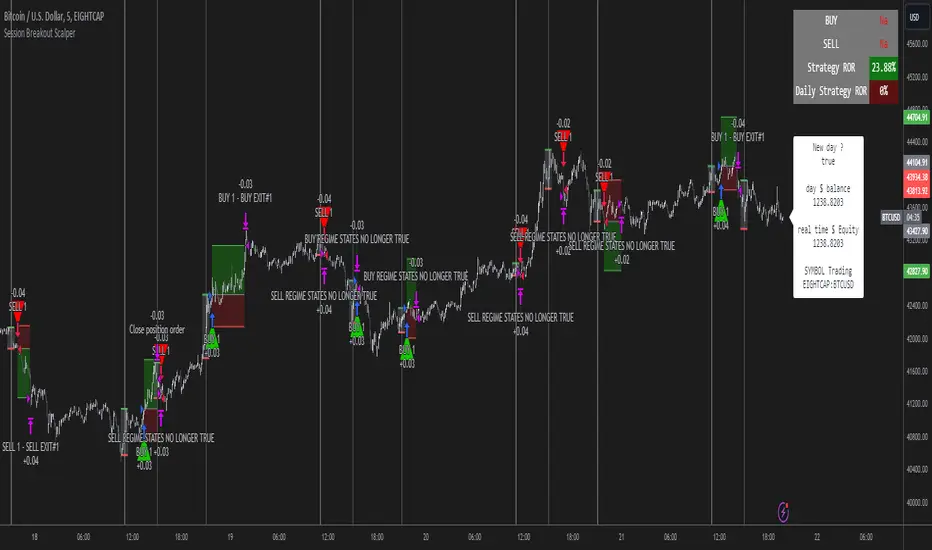
MACD of Relative Strenght StrategyMACD Relative Strenght Strategy :
INTRODUCTION :
This strategy is based on two well-known indicators: MACD and Relative Strenght (RS). By coupling them, we obtain powerful buy signals. In fact, the special feature of this strategy is that it creates an indicator from an indicator. Thus, we construct a MACD whose source is the value of the RS. The strategy only takes buy signals, ignoring SHORT signals as they are mostly losers. There's also a money management method enabling us to reinvest part of the profits or reduce the size of orders in the event of substantial losses.
RELATIVE STRENGHT :
RS is an indicator that measures the anomaly between momentum and the assumption of market efficiency. It is used by professionals and is one of the most robust indicators. The idea is to own assets that do better than average, based on their past performance. We calculate RS using this formula :
RS = close/highest_high(RS_Length)
Where highest_high(RS_Length) = highest value of the high over a user-defined time period (which is the RS_Length).
We can thus situate the current price in relation to its highest price over this user-defined period.
MACD (Moving Average Convergence - Divergence) :
This is one of the best-known indicators, measuring the distance between two exponential moving averages : one fast and one slower. A wide distance indicates fast momentum and vice versa. We'll plot the value of this distance and call this line macdline. The MACD uses a third moving average with a lower period than the first two. This last moving average will give a signal when it crosses the macdline. It is therefore constructed using the values of the macdline as its source.
It's important to note that the first two MAs are constructed using RS values as their source. So we've just built an indicator of an indicator. This kind of method is very powerful because it is rarely used and brings value to the strategy.
PARAMETERS :
RS Length : Relative Strength length i.e. the number of candles back to find the highest high and compare the current price with this high. Default is 300.
MACD Fast Length : Relative Strength fast EMA length used to plot the MACD. Default is 14.
MACD Slow Length : Relative Strength slow EMA length used to plot the MACD. Default is 26.
MACD Signal Smoothing : Macdline SMA length used to plot the MACD. Default is 10.
Max risk per trade (in %) : The maximum loss a trade can incur (in percentage of the trade value). Default is 8%.
Fixed Ratio : This is the amount of gain or loss at which the order quantity is changed. Default is 400, meaning that for each $400 gain or loss, the order size is increased or decreased by a user-selected amount.
Increasing Order Amount : This is the amount to be added to or subtracted from orders when the fixed ratio is reached. The default is $200, which means that for every $400 gain, $200 is reinvested in the strategy. On the other hand, for every $400 loss, the order size is reduced by $200.
Initial capital : $1000
Fees : Interactive Broker fees apply to this strategy. They are set at 0.18% of the trade value.
Slippage : 3 ticks or $0.03 per trade. Corresponds to the latency time between the moment the signal is received and the moment the order is executed by the broker.
Important : A bot has been used to test the different parameters and determine which ones maximize return while limiting drawdown. This strategy is the most optimal on BITSTAMP:ETHUSD in 8h timeframe with the parameters set by default.
ENTER RULES :
The entry rules are very simple : we open a long position when the MACD value turns positive. You are therefore LONG when the MACD is green.
EXIT RULES :
We exit a position (whether losing or winning) when the MACD becomes negative, i.e. turns red.
RISK MANAGEMENT :
This strategy can incur losses, so it's important to manage our risks well. If the position is losing and has incurred a loss of -8%, our stop loss is activated to limit losses.
MONEY MANAGEMENT :
The fixed ratio method was used to manage our gains and losses. For each gain of an amount equal to the value of the fixed ratio, we increase the order size by a value defined by the user in the "Increasing order amount" parameter. Similarly, each time we lose an amount equal to the value of the fixed ratio, we decrease the order size by the same user-defined value. This strategy increases both performance and drawdown.
Enjoy the strategy and don't forget to take the trade :)
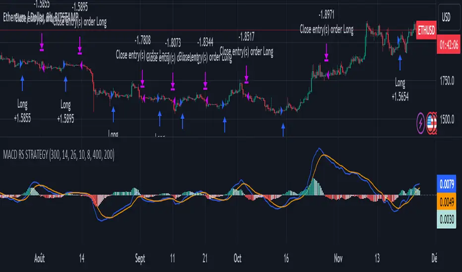
Bollinger Bands StrategyBollinger Bands Strategy :
INTRODUCTION :
This strategy is based on the famous Bollinger Bands. These are constructed using a standard moving average (SMA) and the standard deviation of past prices. The theory goes that 90% of the time, the price is contained between these two bands. If it were to break out, this would mean either a reversal or a continuation. However, when a reversal occurs, the movement is weak, whereas when a continuation occurs, the movement is substantial and profits can be interesting. We're going to use BB to take advantage of this strong upcoming movement, while managing our risks reasonably. There's also a money management method for reinvesting part of the profits or reducing the size of orders in the event of substantial losses.
BOLLINGER BANDS :
The construction of Bollinger bands is straightforward. First, plot the SMA of the price, with a length specified by the user. Then calculate the standard deviation to measure price dispersion in relation to the mean, using this formula :
stdv = (((P1 - avg)^2 + (P2 - avg)^2 + ... + (Pn - avg)^2) / n)^1/2
To plot the two Bollinger bands, we then add a user-defined number of standard deviations to the initial SMA. The default is to add 2. The result is :
Upper_band = SMA + 2*stdv
Lower_band = SMA - 2*stdv
When the price leaves this channel defined by the bands, we obtain buy and sell signals.
PARAMETERS :
BB Length : This is the length of the Bollinger Bands, i.e. the length of the SMA used to plot the bands, and the length of the price series used to calculate the standard deviation. The default is 120.
Standard Deviation Multipler : adds or subtracts this number of times the standard deviation from the initial SMA. Default is 2.
SMA Exit Signal Length : Exit signals for winning and losing trades are triggered by another SMA. This parameter defines the length of this SMA. The default is 110.
Max Risk per trade (in %) : It's the maximum percentage the user can lose in one trade. The default is 6%.
Fixed Ratio : This is the amount of gain or loss at which the order quantity is changed. The default is 400, meaning that for each $400 gain or loss, the order size is increased or decreased by a user-selected amount.
Increasing Order Amount : This is the amount to be added to or subtracted from orders when the fixed ratio is reached. The default is $200, which means that for every $400 gain, $200 is reinvested in the strategy. On the other hand, for every $400 loss, the order size is reduced by $200.
Initial capital : $1000
Fees : Interactive Broker fees apply to this strategy. They are set at 0.18% of the trade value.
Slippage : 3 ticks or $0.03 per trade. Corresponds to the latency time between the moment the signal is received and the moment the order is executed by the broker.
Important : A bot has been used to test the different parameters and determine which ones maximize return while limiting drawdown. This strategy is the most optimal on BITSTAMP:BTCUSD in 8h timeframe with the following parameters :
BB Length = 120
Standard Deviation Multipler = 2
SMA Exit Signal Length = 110
Max Risk per trade (in %) = 6%
ENTER RULES :
The entry rules are simple:
If close > Upper_band it's a LONG signal
If close < Lower_band it's a SHORT signal
EXIT RULES :
If we are LONG and close < SMA_EXIT, position is closed
If we are SHORT and close > SMA_EXIT, the position is closed
Positions close automatically if they lose more than 6% to limit risk
RISK MANAGEMENT :
This strategy is subject to losses. We manage our risk using the exit SMA or using a SL sets to 6%. This SMA gives us exit signals when the price closes below or above, thus limiting losses. If the signal arrives too late, the position is closed after a loss of 6%.
MONEY MANAGEMENT :
The fixed ratio method was used to manage our gains and losses. For each gain of an amount equal to the fixed ratio value, we increase the order size by a value defined by the user in the "Increasing order amount" parameter. Similarly, each time we lose an amount equal to the value of the fixed ratio, we decrease the order size by the same user-defined value. This strategy increases both performance and drawdown.
NOTE :
Please note that the strategy is backtested from 2017-01-01. As the timeframe is 8h, this strategy is a medium/long-term strategy. That's why only 51 trades were closed. Be careful, as the test sample is small and performance may not necessarily reflect what may happen in the future.
Enjoy the strategy and don't forget to take the trade :)

Rate of Change StrategyRate of Change Strategy :
INTRODUCTION :
This strategy is based on the Rate of Change indicator. It compares the current price with that of a user-defined period of time ago. This makes it easy to spot trends and even speculative bubbles. The strategy is long term and very risky, which is why we've added a Stop Loss. There's also a money management method that allows you to reinvest part of your profits or reduce the size of your orders in the event of substantial losses.
RATE OF CHANGE (ROC) :
As explained above, the ROC is used to situate the current price compared to that of a certain period of time ago. The formula for calculating ROC in relation to the previous year is as follows :
ROC (365) = (close/close (365) - 1) * 100
With this formula we can find out how many percent the change in the current price is compared with 365 days ago, and thus assess the trend.
PARAMETERS :
ROC Length : Length of the ROC to be calculated. The current price is compared with that of the selected length ago.
ROC Bubble Signal : ROC value indicating that we are in a bubble. This value varies enormously depending on the financial product. For example, in the equity market, a bubble exists when ROC = 40, whereas in cryptocurrencies, a bubble exists when ROC = 150.
Stop Loss (in %) : Stop Loss value in percentage. This is the maximum trade value percentage that can be lost in a single trade.
Fixed Ratio : This is the amount of gain or loss at which the order quantity is changed. The default is 400, which means that for each $400 gain or loss, the order size is increased or decreased by an amount chosen by the user.
Increasing Order Amount : This is the amount to be added to or subtracted from orders when the fixed ratio is reached. The default is $200, which means that for every $400 gain, $200 is reinvested in the strategy. On the other hand, for every $400 loss, the order size is reduced by $200.
Initial capital : $1000
Fees : Interactive Broker fees apply to this strategy. They are set at 0.18% of the trade value.
Slippage : 3 ticks or $0.03 per trade. Corresponds to the latency time between the moment the signal is received and the moment the order is executed by the broker.
Important : A bot has been used to test the different parameters and determine which ones maximize return while limiting drawdown. This strategy is the most optimal on BITSTAMP:BTCUSD in 1D timeframe with the following parameters :
ROC Length = 365
ROC Bubble Signal = 180
Stop Loss (in %) = 6
LONG CONDITION :
We are in a LONG position if ROC (365) > 0 for at least two days. This allows us to limit noise and irrelevant signals to ensure that the ROC remains positive.
SHORT CONDITION :
We are in a SHORT position if ROC (365) < 0 for at least two days. We also open a SHORT position when the speculative bubble is about to burst. If ROC (365) > 180, we're in a bubble. If the bubble has been in existence for at least a week and the ROC falls back below this threshold, we can expect the asset to return to reasonable prices, and thus a downward trend. So we're opening a SHORT position to take advantage of this upcoming decline.
EXIT RULES FOR WINNING TRADE :
The strategy is self-regulating. We don't exit a LONG trade until a SHORT signal has arrived, and vice versa. So, to exit a winning position, you have to wait for the entry signal of the opposite position.
RISK MANAGEMENT :
This strategy is very risky, and we can easily end up on the wrong side of the trade. That's why we're going to manage our risk with a Stop Loss, limiting our losses as a percentage of the trade's value. By default, this percentage is set at 6%. Each trade will therefore take a maximum loss of 6%.
If the SL has been triggered, it probably means we were on the wrong side. This is why we change the direction of the trade when a SL is triggered. For example, if we were SHORT and lost 6% of the trade value, the strategy will close this losing trade and open a long position without taking into account the ROC value. This allows us to be in position all the time and not miss the best opportunities.
MONEY MANAGEMENT :
The fixed ratio method was used to manage our gains and losses. For each gain of an amount equal to the value of the fixed ratio, we increase the order size by a value defined by the user in the "Increasing order amount" parameter. Similarly, each time we lose an amount equal to the value of the fixed ratio, we decrease the order size by the same user-defined value. This strategy increases both performance and drawdown.
NOTE :
Please note that the strategy is backtested from 2017-01-01. As the timeframe is 1D, this strategy is a medium/long-term strategy. That's why only 34 trades were closed. Be careful, as the test sample is small and performance may not necessarily reflect what may happen in the future.
Enjoy the strategy and don't forget to take the trade :)

RSI & Backed-Weighted MA StrategyRSI & MA Strategy :
INTRODUCTION :
This strategy is based on two well-known indicators that work best together: the Relative Strength Index (RSI) and the Moving Average (MA). We're going to use the RSI as a trend-follower indicator, rather than a reversal indicator as most are used to. To the signals sent by the RSI, we'll add a condition on the chart's MA, filtering out irrelevant signals and considerably increasing our winning rate. This is a medium/long-term strategy. There's also a money management method enabling us to reinvest part of the profits or reduce the size of orders in the event of substantial losses.
RSI :
The RSI is one of the best-known and most widely used indicators in trading. Its purpose is to warn traders when an asset is overbought or oversold. It was designed to send reversal signals, but we're going to use it as a trend indicator by increasing its length to 20. The RSI formula is as follows :
RSI (n) = 100 - (100 / (1 + (H (n)/L (n))))
With n the length of the RSI, H(n) the average of days closing above the open and L(n) the average of days closing below the open.
MA :
The Moving Average is also widely used in technical analysis, to smooth out variations in an asset. The SMA formula is as follows :
SMA (n) = (P1 + P2 + ... + Pn) / n
where n is the length of the MA.
However, an SMA does not weight any of its terms, which means that the price 10 days ago has the same importance as the price 2 days ago or today's price... That's why in this strategy we use a RWMA, i.e. a back-weighted moving average. It weights old prices more heavily than new ones. This will enable us to limit the impact of short-term variations and focus on the trend that was dominating. The RWMA used weights :
The 4 most recent terms by : 100 / (4+(n-4)*1.30)
The other oldest terms by : weight_4_first_term*1.30
So the older terms are weighted 1.30 more than the more recent ones. The moving average thus traces a trend that accentuates past values and limits the noise of short-term variations.
PARAMETERS :
RSI Length : Lenght of RSI. Default is 20.
MA Type : Choice between a SMA or a RWMA which permits to minimize the impact of short term reversal. Default is RWMA.
MA Length : Length of the selected MA. Default is 19.
RSI Long Signal : Minimum value of RSI to send a LONG signal. Default is 60.
RSI Short signal : Maximum value of RSI to send a SHORT signal. Default is 40.
ROC MA Long Signal : Maximum value of Rate of Change MA to send a LONG signal. Default is 0.
ROC MA Short signal : Minimum value of Rate of Change MA to send a SHORT signal. Default is 0.
TP activation in multiple of ATR : Threshold value to trigger trailing stop Take Profit. This threshold is calculated as multiple of the ATR (Average True Range). Default value is 5 meaning that to trigger the trailing TP the price need to move 5*ATR in the right direction.
Trailing TP in percentage : Percentage value of trailing Take Profit. This Trailing TP follows the profit if it increases, remaining selected percentage below it, but stops if the profit decreases. Default is 3%.
Fixed Ratio : This is the amount of gain or loss at which the order quantity is changed. Default is 400, which means that for each $400 gain or loss, the order size is increased or decreased by a user-selected amount.
Increasing Order Amount : This is the amount to be added to or subtracted from orders when the fixed ratio is reached. The default is $200, which means that for every $400 gain, $200 is reinvested in the strategy. On the other hand, for every $400 loss, the order size is reduced by $200.
Initial capital : $1000
Fees : Interactive Broker fees apply to this strategy. They are set at 0.18% of the trade value.
Slippage : 3 ticks or $0.03 per trade. Corresponds to the latency time between the moment the signal is received and the moment the order is executed by the broker.
Important : A bot has been used to test the different parameters and determine which ones maximize return while limiting drawdown. This strategy is the most optimal on BITSTAMP:ETHUSD with a timeframe set to 6h. Parameters are set as follows :
MA type: RWMA
MA Length: 19
RSI Long Signal: >60
RSI Short Signal : <40
ROC MA Long Signal : <0
ROC MA Short Signal : >0
TP Activation in multiple ATR : 5
Trailing TP in percentage : 3
ENTER RULES :
The principle is very simple:
If the asset is overbought after a bear market, we are LONG.
If the asset is oversold after a bull market, we are SHORT.
We have defined a bear market as follows : Rate of Change (20) RWMA < 0
We have defined a bull market as follows : Rate of Change (20) RWMA > 0
The Rate of Change is calculated using this formula : (RWMA/RWMA(20) - 1)*100
Overbought is defined as follows : RSI > 60
Oversold is defined as follows : RSI < 40
LONG CONDITION :
RSI > 60 and (RWMA/RWMA(20) - 1)*100 < -1
SHORT CONDITION :
RSI < 40 and (RWMA/RWMA(20) - 1)*100 > 1
EXIT RULES FOR WINNING TRADE :
We have a trailing TP allowing us to exit once the price has reached the "TP Activation in multiple ATR" parameter, i.e. 5*ATR by default in the profit direction. TP trailing is triggered at this point, not limiting our gains, and securing our profits at 3% below this trigger threshold.
Remember that the True Range is : maximum(H-L, H-C(1), C-L(1))
with C : Close, H : High, L : Low
The Average True Range is therefore the average of these TRs over a length defined by default in the strategy, i.e. 20.
RISK MANAGEMENT :
This strategy may incur losses. The method for limiting losses is to set a Stop Loss equal to 3*ATR. This means that if the price moves against our position and reaches three times the ATR, we exit with a loss.
Sometimes the ATR can result in a SL set below 10% of the trade value, which is not acceptable. In this case, we set the SL at 10%, limiting losses to a maximum of 10%.
MONEY MANAGEMENT :
The fixed ratio method was used to manage our gains and losses. For each gain of an amount equal to the value of the fixed ratio, we increase the order size by a value defined by the user in the "Increasing order amount" parameter. Similarly, each time we lose an amount equal to the value of the fixed ratio, we decrease the order size by the same user-defined value. This strategy increases both performance and drawdown.
Enjoy the strategy and don't forget to take the trade :)