Market Imbalance Tracker (Inefficient Candle + FVG)# 📊 Overview
This indicator combines two imbalance concepts:
• **Squared Up Points (SUP)** – midpoints of large, "inefficient" candles that often attract price back.
• **Fair Value Gaps (FVG)** – 3-candle gaps created by strong impulse moves that often get "filled."
Use them separately or together. Confluence between a SUP line and an FVG boundary/midpoint is high-value.
---
# ⚡ Quick Start (2 minutes)
1. **Add to chart** → keep defaults (Percentile method, 80th percentile, 100-bar lookback).
2. **Watch** for dashed SUP lines to print after large candles.
3. **Toggle Show FVG** → see green/red boxes where gaps exist.
4. **Turn on alerts** → New SUP created, SUP touched, New FVG.
5. **Trade the reaction** → look for confluence (SUP + FVG + S/R), then manage risk.
---
# 🛠 Features
## 🔹 Squared Up Points (SUP)
• **Purpose:** Midpoint of a large candle → potential support/resistance magnet.
• **Detection:** Choose *Percentile* (adaptive) or *ATR Multiple* (absolute).
• **Validation:** Only plots if the preceding candle does not touch the midpoint (with tolerance).
• **Lifecycle:** Line auto-extends into the future; it's removed when touched or aged out.
• **Visual:** Horizontal dashed line (color/width configurable; style fixed to dashed if not exposed).
## 🔹 Fair Value Gaps (FVG)
• **Purpose:** 3-candle gaps from an impulse; price often revisits to "fill."
• **Detection:** Requires a strong directional candle (Marubozu threshold) creating a gap.
• **Types:**
- **Bullish FVG (Green):** Gap below; expectation is downward fill.
- **Bearish FVG (Red):** Gap above; expectation is upward fill.
• **Close Rules (if implemented):**
- *Full Fill:* Gap closes when the opposite boundary is tagged.
- *Midpoint Fill:* Gap closes when its midpoint is tagged.
• **Visual:** Colored boxes; optional split-coloring to emphasize the midpoint.
> **Note:** If a listed FVG option isn't visible in Inputs, you're on a lighter build; use the available switches.
---
# ⚙️ Settings
## SUP Settings
• **Candle Size Method:** Percentile (top X% of recent ranges) or ATR Multiple.
• **Candle Size Percentile:** e.g., 80 → top 20% largest candles.
• **ATR Multiple & Period:** e.g., 1.5 × ATR(14).
• **Percentile Lookback:** Bars used to compute percentile.
• **Lookback Period:** How long SUP lines remain eligible before auto-cleanup.
• **Touch Tolerance (%):** Buffer based on the inefficient candle's range (0% = exact touch).
## Line Appearance
• **Line Color / Width:** Customizable.
• **Style:** Dashed (fixed unless you expose a style input).
## FVG Settings (if present in your build)
• **Show FVG:** On/Off.
• **Close Method:** Full Fill or Midpoint.
• **Marubozu Wick Tolerance:** Max wick % of the impulse bar.
• **Use Split Coloring:** Two-tone box halves around midpoint.
• **Colors:** Bullish/Bearish, and upper/lower halves (if split).
• **Max FVG Age:** Auto-remove older gaps.
---
# 📈 How to Use
## Trading Applications
• **SUP Lines:** Expect reaction on first touch; use as S/R or profit-taking magnets.
• **FVG Fills:** Price frequently tags the midpoint/boundary before continuing.
• **Confluence:** SUP at an FVG midpoint/boundary + higher-timeframe S/R = higher quality.
• **Bias:** Clusters of unfilled FVGs can hint at path of least resistance.
## Best Practices
• **Timeframe:** HTFs for swing levels, LTFs for execution.
• **Volume:** High volume at level = stronger signal.
• **Context:** Trade with broader trend or at least avoid counter-trend without confirmation.
• **Risk:** Always pre-define invalidation; structures fail in chop.
---
# 🔔 Alerts
• **New SUP Created** – When a qualifying inefficient candle prints a SUP midpoint.
• **SUP Touched/Invalidated** – When price touches within tolerance.
• **New FVG Detected** – When a valid gap forms per your rules.
> **Tip:** Set alerts *Once Per Bar Close* on HTFs; *Once* on LTFs to avoid noise.
---
# 🧑💻 Technical Notes
• **Percentile vs ATR:** Percentile adapts to volatility; ATR gives consistency for backtesting.
• **FVG Direction Logic:** Gap above price = bearish (expect up-fill); below = bullish (expect down-fill).
• **Performance:** Limits on lines/boxes and auto-aging keep things snappy.
---
# ⚠️ Limitations
• Imbalances are **context tools**, not signals by themselves.
• Works best with trend or clear impulses; expect noise in narrow ranges.
• Lower-timeframe gaps can be plentiful and lower quality.
---
# 📌 Version & Requirements
• **Pine Script v6**
• Heavy drawings may require **TradingView Pro** or higher (object limits).
---
*For best results, combine with your existing trading strategy and proper risk management.*
Pesquisar nos scripts por "backtesting"

Hurst Exponent Adaptive Filter (HEAF) [PhenLabs]📊 PhenLabs - Hurst Exponent Adaptive Filter (HEAF)
Version: PineScript™ v6
📌 Description
The Hurst Exponent Adaptive Filter (HEAF) is an advanced Pine Script indicator designed to dynamically adjust moving average calculations based on real time market regimes detected through the Hurst Exponent. The intention behind the creation of this indicator was not a buy/sell indicator but rather a tool to help sharpen traders ability to distinguish regimes in the market mathematically rather than guessing. By analyzing price persistence, it identifies whether the market is trending, mean-reverting, or exhibiting random walk behavior, automatically adapting the MA length to provide more responsive alerts in volatile conditions and smoother outputs in stable ones. This helps traders avoid false signals in choppy markets and capitalize on strong trends, making it ideal for adaptive trading strategies across various timeframes and assets.
Unlike traditional moving averages, HEAF incorporates fractal dimension analysis via the Hurst Exponent to create a self-tuning filter that evolves with market conditions. Traders benefit from visual cues like color coded regimes, adaptive bands for volatility channels, and an information panel that suggests appropriate strategies, enhancing decision making without constant manual adjustments by the user.
🚀 Points of Innovation
Dynamic MA length adjustment using Hurst Exponent for regime-aware filtering, reducing lag in trends and noise in ranges.
Integrated market regime classification (trending, mean-reverting, random) with visual and alert-based notifications.
Customizable color themes and adaptive bands that incorporate ATR for volatility-adjusted channels.
Built-in information panel providing real-time strategy recommendations based on detected regimes.
Power sensitivity parameter to fine-tune adaptation aggressiveness, allowing personalization for different trading styles.
Support for multiple MA types (EMA, SMA, WMA) within an adaptive framework.
🔧 Core Components
Hurst Exponent Calculation: Computes the fractal dimension of price series over a user-defined lookback to detect market persistence or anti-persistence.
Adaptive Length Mechanism: Maps Hurst values to MA lengths between minimum and maximum bounds, using a power function for sensitivity control.
Moving Average Engine: Applies the chosen MA type (EMA, SMA, or WMA) to the adaptive length for the core filter line.
Adaptive Bands: Creates upper and lower channels using ATR multiplied by a band factor, scaled to the current adaptive length.
Regime Detection: Classifies market state with thresholds (e.g., >0.55 for trending) and triggers alerts on regime changes.
Visualization System: Includes gradient fills, regime-colored MA lines, and an info panel for at-a-glance insights.
🔥 Key Features
Regime-Adaptive Filtering: Automatically shortens MA in mean-reverting markets for quick responses and lengthens it in trends for smoother signals, helping traders stay aligned with market dynamics.
Custom Alerts: Notifies on regime shifts and band breakouts, enabling timely strategy adjustments like switching to trend-following in bullish regimes.
Visual Enhancements: Color-coded MA lines, gradient band fills, and an optional info panel that displays market state and trading tips, improving chart readability.
Flexible Settings: Adjustable lookback, min/max lengths, sensitivity power, MA type, and themes to suit various assets and timeframes.
Band Breakout Signals: Highlights potential overbought/oversold conditions via ATR-based channels, useful for entry/exit timing.
🎨 Visualization
Main Adaptive MA Line: Plotted with regime-based colors (e.g., green for trending) to visually indicate market state and filter position relative to price.
Adaptive Bands: Upper and lower lines with gradient fills between them, showing volatility channels that widen in random regimes and tighten in trends.
Price vs. MA Fills: Color-coded areas between price and MA (e.g., bullish green above MA in trending modes) for quick trend strength assessment.
Information Panel: Top-right table displaying current regime (e.g., "Trending Market") and strategy suggestions like "Follow trends" or "Trade ranges."
📖 Usage Guidelines
Core Settings
Hurst Lookback Period
Default: 100
Range: 20-500
Description: Sets the period for Hurst Exponent calculation; longer values provide more stable regime detection but may lag, while shorter ones are more responsive to recent changes.
Minimum MA Length
Default: 10
Range: 5-50
Description: Defines the shortest possible adaptive MA length, ideal for fast responses in mean-reverting conditions.
Maximum MA Length
Default: 200
Range: 50-500
Description: Sets the longest adaptive MA length for smoothing in strong trends; adjust based on asset volatility.
Sensitivity Power
Default: 2.0
Range: 1.0-5.0
Description: Controls how aggressively the length adapts to Hurst changes; higher values make it more sensitive to regime shifts.
MA Type
Default: EMA
Options: EMA, SMA, WMA
Description: Chooses the moving average calculation method; EMA is more responsive, while SMA/WMA offer different weighting.
🖼️ Visual Settings
Show Adaptive Bands
Default: True
Description: Toggles visibility of upper/lower bands for volatility channels.
Band Multiplier
Default: 1.5
Range: 0.5-3.0
Description: Scales band width using ATR; higher values create wider channels for conservative signals.
Show Information Panel
Default: True
Description: Displays regime info and strategy tips in a top-right panel.
MA Line Width
Default: 2
Range: 1-5
Description: Adjusts thickness of the main MA line for better visibility.
Color Theme
Default: Blue
Options: Blue, Classic, Dark Purple, Vibrant
Description: Selects color scheme for MA, bands, and fills to match user preferences.
🚨 Alert Settings
Enable Alerts
Default: True
Description: Activates notifications for regime changes and band breakouts.
✅ Best Use Cases
Trend-Following Strategies: In detected trending regimes, use the adaptive MA as a trailing stop or entry filter for momentum trades.
Range Trading: During mean-reverting periods, monitor band breakouts for buying dips or selling rallies within channels.
Risk Management in Random Markets: Reduce exposure when random walk is detected, using tight stops suggested in the info panel.
Multi-Timeframe Analysis: Apply on higher timeframes for regime confirmation, then drill down to lower ones for entries.
Volatility-Based Entries: Use upper/lower band crossovers as signals in adaptive channels for overbought/oversold trades.
⚠️ Limitations
Lagging in Transitions: Regime detection may delay during rapid market shifts, requiring confirmation from other tools.
Not a Standalone System: Best used in conjunction with other indicators; random regimes can lead to whipsaws if traded aggressively.
Parameter Sensitivity: Optimal settings vary by asset and timeframe, necessitating backtesting.
💡 What Makes This Unique
Hurst-Driven Adaptation: Unlike static MAs, it uses fractal analysis to self-tune, providing regime-specific filtering that's rare in standard indicators.
Integrated Strategy Guidance: The info panel offers actionable tips tied to regimes, bridging analysis and execution.
Multi-Regime Visualization: Combines adaptive bands, colored fills, and alerts in one tool for comprehensive market state awareness.
🔬 How It Works
Hurst Exponent Computation:
Calculates log returns over the lookback period to derive the rescaled range (R/S) ratio.
Normalizes to a 0-1 value, where >0.55 indicates trending, <0.45 mean-reverting, and in-between random.
Length Adaptation:
Maps normalized Hurst to an MA length via a power function, clamping between min and max.
Applies the selected MA type to close prices using this dynamic length.
Visualization and Signals:
Plots the MA with regime colors, adds ATR-based bands, and fills areas for trend strength.
Triggers alerts on regime changes or band crosses, with the info panel suggesting strategies like momentum riding in trends.
💡 Note:
For optimal results, backtest settings on your preferred assets and combine with volume or momentum indicators. Remember, no indicator guarantees profits—use with proper risk management. Access premium features and support at PhenLabs.

Intraday Momentum StrategyExplanation of the StrategyIndicators:Fast and Slow EMA: A crossover of the 9-period EMA over the 21-period EMA signals a bullish trend (long entry), while a crossunder signals a bearish trend (short entry).
RSI: Ensures entries are not in overbought (RSI > 70) or oversold (RSI < 30) conditions to avoid reversals.
VWAP: Acts as a dynamic support/resistance. Long entries require the price to be above VWAP, and short entries require it to be below.
Trading Session:The strategy only trades during a user-defined session (e.g., 9:30 AM to 3:45 PM, typical for US markets).
All positions are closed at the session end to avoid overnight risk.
Risk Management:Stop Loss: 1% below/above the entry price for long/short positions.
Take Profit: 2% above/below the entry price for long/short positions.
These can be adjusted via inputs for optimization.
Position Sizing:Fixed lot size of 1 for simplicity. Adjust based on your account size during backtesting.

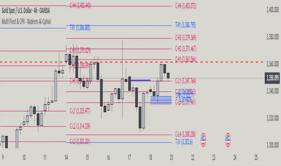
Multi Pivot Point & Central Pivot Range - Nadeem Al-QahwiThis indicator combines four advanced trading modules into one flexible and easy-to-use script:
Traditional Pivot Points:
Calculates classic support and resistance levels (PP, R1–R5, S1–S5) based on previous session data. Ideal for identifying key turning points and mapping out the daily, weekly, or monthly structure.
Camarilla Levels:
Provides six upper and lower pivot levels (H1–H6, L1–L6) derived from volatility and closing price formulas. Especially effective for intraday reversal, mean reversion, and finding overbought/oversold extremes.
Central Pivot Range (CPR):
Plots the median, top, and bottom of the value area each session. CPR width instantly highlights whether the market is likely to trend (narrow CPR) or remain range-bound (wide CPR).
Developing CPR projects the evolving range for the current period—essential for real-time analysis and pre-market planning.
Dynamic Zone Levels (DZL):
Automatically detects and highlights clusters of pivots to reveal high-probability support/resistance zones, filtering out market “noise.”
DZL alerts notify you whenever price breaks or retests these key areas, making it easier to spot momentum trades and avoid false signals.
Key Features:
Multi-timeframe flexibility: Use with daily, weekly, monthly, yearly, or custom timeframes—even rare ones like biyearly and decennial.
Modular design: Activate or hide any system (Traditional, Camarilla, CPR, DZL) as you need.
Bilingual interface: Every setting and label is shown in both English and Arabic.
Full customization: Control visibility, color, style, and placement for every level and label.
Historical depth: Plot up to 5,000 pivot/zones back for deep analysis and backtesting.
Smart alerts: Get instant notifications on true S/R breakouts or retests (from DZL).
How to Use:
Trend Trading:
Watch for a very narrow CPR to identify potential trending days—trade in the breakout direction above/below the CPR.
Range Trading:
When CPR is wide, expect sideways movement. Fade reversals at R1/S1 or within the CPR boundaries.
Breakouts:
Use DZL alerts to capture momentum as price breaks or retests dynamic support/resistance zones.
Multi-Timeframe Confluence:
Combine CPR and pivot levels from multiple timeframes for higher-probability entries and exits.
All calculations and logic are fully open.
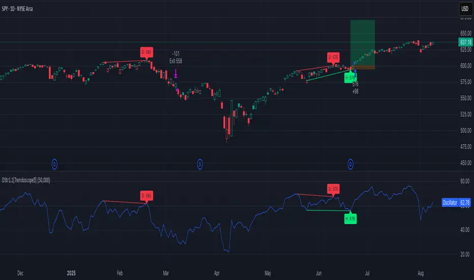
Divergence Strategy [Trendoscope®]🎲 Overview
The Divergence Strategy is a sophisticated TradingView strategy that enhances the Divergence Screener by adding automated trade signal generation, risk management, and trade visualization. It leverages the screener’s robust divergence detection to identify bullish, bearish, regular, and hidden divergences, then executes trades with precise entry, stop-loss, and take-profit levels. Designed for traders seeking automated trading solutions, this strategy offers customizable trade parameters and visual feedback to optimize performance across various markets and timeframes.
For core divergence detection features, including oscillator options, trend detection methods, zigzag pivot analysis, and visualization, refer to the Divergence Screener documentation. This description focuses on the strategy-specific enhancements for automated trading and risk management.
🎲 Strategy Features
🎯Automated Trade Signal Generation
Trade Direction Control : Restrict trades to long-only or short-only to align with market bias or strategy goals, preventing conflicting orders.
Divergence Type Selection : Choose to trade regular divergences (bullish/bearish), hidden divergences, or both, targeting reversals or trend continuations.
Entry Type Options :
Cautious : Enters conservatively at pivot points and exits quickly to minimize risk exposure.
Confident : Enters aggressively at the latest price and holds longer to capture larger moves.
Mixed : Combines conservative entries with delayed exits for a balanced approach.
Market vs. Stop Orders: Opt for market orders for instant execution or stop orders for precise price entry.
🎯 Enhanced Risk Management
Risk/Reward Ratio : Define a risk-reward ratio (default: 2.0) to set profit targets relative to stop-loss levels, ensuring consistent trade sizing.
Bracket Orders : Trades include entry, stop-loss, and take-profit levels calculated from divergence pivot points, tailored to the entry type and risk-reward settings.
Stop-Loss Placement : Stops are strategically set (e.g., at recent pivot or last price point) based on entry type, balancing risk and trade validity.
Order Cancellation : Optionally cancel pending orders when a divergence is broken (e.g., price moves past the pivot in the wrong direction), reducing invalid trades. This feature is toggleable for flexibility.
🎯 Trade Visualization
Target and Stop Boxes : Displays take-profit (lime) and stop-loss (orange) levels as boxes on the price chart, extending 10 bars forward for clear visibility.
Dynamic Trade Updates : Trade visualizations are added, updated, or removed as trades are executed, canceled, or invalidated, ensuring accurate feedback.
Overlay Integration : Trade levels overlay the price chart, complementing the screener’s oscillator-based divergence lines and labels.
🎯 Strategy Default Configuration
Capital and Sizing : Set initial capital (default: $1,000,000) and position size (default: 20% of equity) for realistic backtesting.
Pyramiding : Allows up to 4 concurrent trades, enabling multiple divergence-based entries in trending markets.
Commission and Margin : Accounts for commission (default: 0.01%) and margin (100% for long/short) to reflect trading costs.
Performance Optimization : Processes up to 5,000 bars dynamically, balancing historical analysis and real-time execution.
🎲 Inputs and Configuration
🎯Trade Settings
Direction : Select Long or Short (default: Long).
Divergence : Trade Regular, Hidden, or Both divergence types (default: Both).
Entry/Exit Type : Choose Cautious, Confident, or Mixed (default: Cautious).
Risk/Reward : Set the risk-reward ratio for profit targets (default: 2.0).
Use Market Order : Enable market orders for immediate entry (default: false, uses limit orders).
Cancel On Break : Cancel pending orders when divergence is broken (default: true).
🎯Inherited Settings
The strategy inherits all inputs from the Divergence Screener, including:
Oscillator Settings : Oscillator type (e.g., RSI, CCI), length, and external oscillator option.
Trend Settings : Trend detection method (Zigzag, MA Difference, External), MA type, and length.
Zigzag Settings : Zigzag length (fixed repaint = true).
🎲 Entry/Exit Types for Divergence Scenarios
The Divergence Strategy offers three Entry/Exit Type options—Cautious, Confident, and Mixed—which determine how trades are entered and exited based on divergence pivot points. This section explains how these settings apply to different divergence scenarios, with placeholders for screenshots to illustrate each case.
The divergence pattern forms after 3 pivots. The stop and entry levels are formed on one of these levels based on Entry/Exit types.
🎯Bullish Divergence (Reversal)
A bullish divergence occurs when price forms a lower low, but the oscillator forms a higher low, signaling a potential upward reversal.
💎 Cautious:
Entry : At the pivot high point for a conservative entry.
Exit : Stop-loss at the last pivot point (previous low that is higher than the current pivot low); take-profit at risk-reward ratio. Canceled if price breaks below the pivot (if Cancel On Break is enabled).
Behavior : Enters after confirmation and exits quickly to limit downside risk.
💎Confident:
Entry : At the last pivot low, (previous low which is higher than the current pivot low) for an aggressive entry.
Exit : Stop-loss at recent pivot low, which is the lowest point; take-profit at risk-reward ratio. Canceled if price breaks below the pivot. (lazy exit)
Behavior : Enters early to capture trend continuation, holding longer for gains.
💎Mixed:
Entry : At the pivot high point (conservative).
Exit : Stop-loss at the recent pivot point that has resulted in lower low (lazy exit). Canceled if price breaks below the pivot.
Behavior : Balances entry caution with extended holding for trend continuation.
🎯Bearish Divergence (Reversal)
A bearish divergence occurs when price forms a higher high, but the oscillator forms a lower high, indicating a potential downward reversal.
💎Cautious:
Entry : At the pivot low point (lower high) for a conservative short entry.
Exit : Stop-loss at the previous pivot high point (previous high); take-profit at risk-reward ratio. Canceled if price breaks above the pivot (if Cancel On Break is enabled).
Behavior : Enters conservatively and exits quickly to minimize risk.
💎Confident:
Entry : At the last price point (previous high) for an aggressive short entry.
Exit : Stop-loss at the pivot point; take-profit at risk-reward ratio. Canceled if price breaks above the pivot.
Behavior : Enters early to maximize trend continuation, holding longer.
💎Mixed:
Entry : At the previous piot high point (conservative).
Exit : Stop-loss at the last price point (delayed exit). Canceled if price breaks above the pivot.
Behavior : Combines conservative entry with extended holding for downtrend gains.
🎯Bullish Hidden Divergence (Continuation)
A bullish hidden divergence occurs when price forms a higher low, but the oscillator forms a lower low, suggesting uptrend continuation. In case of Hidden bullish divergence, b]Entry is always on the previous pivot high (unless it is a market order)
💎Cautious:
Exit : Stop-loss at the recent pivot low point (higher than previous pivot low); take-profit at risk-reward ratio. Canceled if price breaks below the pivot (if Cancel On Break is enabled).
Behavior : Enters after confirmation and exits quickly to limit downside risk.
💎Confident:
Exit : Stop-loss at previous pivot low, which is the lowest point; take-profit at risk-reward ratio. Canceled if price breaks below the pivot. (lazy exit)
Behavior : Enters early to capture trend continuation, holding longer for gains.
🎯Bearish Hidden Divergence (Continuation)
A bearish hidden divergence occurs when price forms a lower high, but the oscillator forms a higher high, suggesting downtrend continuation. In case of Hidden Bearish divergence, b]Entry is always on the previous pivot low (unless it is a market order)
💎Cautious:
Exit : Stop-loss at the latest pivot high point (which is a lower high); take-profit at risk-reward ratio. Canceled if price breaks above the pivot (if Cancel On Break is enabled).
Behavior : Enters conservatively and exits quickly to minimize risk.
💎Confident/Mixed:
Exit : Stop-loss at the previous pivot high point; take-profit at risk-reward ratio. Canceled if price breaks above the pivot.
Behavior : Uses the late exit point to hold longer.
🎲 Usage Instructions
🎯Add to Chart:
Add the Divergence Strategy to your TradingView chart.
The oscillator and divergence signals appear in a separate pane, with trade levels (target/stop boxes) overlaid on the price chart.
🎯Configure Settings:
Adjust trade settings (direction, divergence type, entry type, risk-reward, market orders, cancel on break).
Modify inherited Divergence Screener settings (oscillator, trend method, zigzag length) as needed.
Enable/disable alerts for divergence notifications.
🎯Interpret Signals:
Long Trades: Triggered on bullish or bullish hidden divergences (if allowed), shown with green/lime lines and labels.
Short Trades: Triggered on bearish or bearish hidden divergences (if allowed), shown with red/orange lines and labels.
Monitor lime (target) and orange (stop) boxes for trade levels.
Review strategy performance metrics (e.g., profit/loss, win rate) in the strategy tester.
🎯Backtest and Optimize:
Use TradingView’s strategy tester to evaluate performance on historical data.
Fine-tune risk-reward, entry type, position sizing, and cancellation settings to suit your market and timeframe.
For questions, suggestions, or support, contact Trendoscope via TradingView or official support channels. Stay tuned for updates and enhancements to the Divergence Strategy!
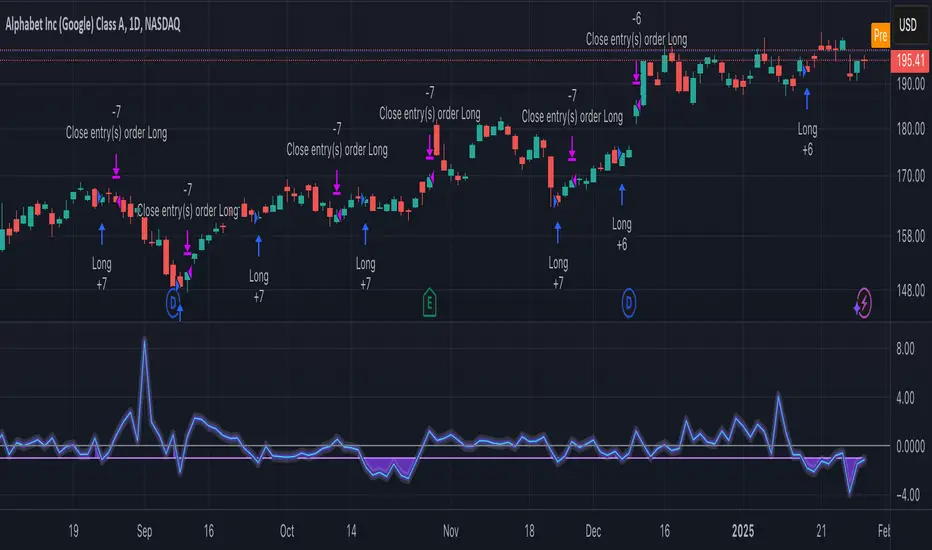
GCM Bull Bear RiderGCM Bull Bear Rider (GCM BBR)
Your Ultimate Trend-Riding Companion
GCM Bull Bear Rider is a comprehensive, all-in-one trend analysis tool designed to eliminate guesswork and provide a crystal-clear view of market direction. By leveraging a highly responsive Jurik Moving Average (JMA), this indicator not only identifies bullish and bearish trends with precision but also tracks their performance in real-time, helping you ride the waves of momentum from start to finish.
Whether you are a scalper, day trader, or swing trader, the GCM BBR adapts to your style, offering a clean, intuitive, and powerful visual guide to the market's pulse.
Key Features
JMA-Powered Trend Lines (UTPL & DTPL): The core of the indicator. A green "Up Trend Period Line" (UTPL) appears when the JMA's slope turns positive (buyers are in control), and a red "Down Trend Period Line" (DTPL) appears when the slope turns negative (sellers are in control). The JMA is used for its low lag and superior smoothing, giving you timely and reliable trend signals.
Live Profit Tracking Labels: This is the standout feature. As soon as a trend period begins, a label appears showing the real-time profit (P:) from the trend's starting price. This label moves with the trend, giving you instant feedback on its performance and helping you make informed trade management decisions.
Historical Performance Analysis: The profit labels remain on the chart for completed trends, allowing you to instantly review past performance. See at a glance which trends were profitable and which were not, aiding in strategy refinement and backtesting.
Automatic Chart Decluttering: To keep your chart clean and focused on significant moves, the indicator automatically removes the historical profit label for any trend that fails to achieve a minimum profit threshold (default is 0.5 points).
Dual-Ribbon Momentum System:
JMA / Short EMA Ribbon: Visualizes short-term momentum. A green fill indicates immediate bullish strength, while a red fill shows bearish pressure.
Short EMA / Long EMA Ribbon: Acts as a long-term trend filter, providing broader market context for your decisions.
"GCM Hunt" Entry Signals: The indicator includes optional pullback entry signals (green and red triangles). These appear when the price pulls back to a key moving average and then recovers in the direction of the primary trend, offering high-probability entry opportunities.
How to Use
Identify the Trend: Look for the appearance of a solid green line (UTPL) for a bullish bias or a solid red line (DTPL) for a bearish bias. Use the wider EMA ribbon for macro trend confirmation.
Time Your Entry: For aggressive entries, you can enter as soon as a new trend line appears. For more conservative entries, wait for a "GCM Hunt" triangle signal, which confirms a successful pullback.
Ride the Trend & Manage Your Trade: The moving profit label (P:) is your guide. As long as the trend line continues and the profit is increasing, you can confidently stay in the trade. A flattening JMA or a decreasing profit value can signal that the trend is losing steam.
Focus Your Strategy: Use the Display Mode setting to switch between "Buyers Only," "Sellers Only," or both. This allows you to completely hide opposing signals and focus solely on long or short opportunities.
Core Settings
Display Mode: The master switch. Choose to see visuals for "Buyers & Sellers," "Buyers Only," or "Sellers Only."
JMA Settings (Length, Phase): Fine-tune the responsiveness of the core JMA engine.
EMA Settings (Long, Short): Adjust the lengths of the moving averages that define the ribbons and "Hunt" signals.
Label Offset (ATR Multiplier): Customize the gap between the trend lines and the profit labels to avoid overlap with candles.
Filters (EMA, RSI, ATR, Strong Candle): Enable or disable various confirmation filters to strengthen the "Hunt" entry signals according to your risk tolerance.
Add the GCM Bull Bear Rider to your chart today and transform the way you see and trade the trend!
ENJOY

ATR Buy, Target, Stop + OverlayATR Buy, Target, Stop + Overlay
This tool is to assist traders with precise trade planning using the Average True Range (ATR) as a volatility-based reference.
This script plots buy, target, and stop-loss levels on the chart based on a user-defined buy price and ATR-based multipliers, allowing for objective and adaptive trade management.
*NOTE* In order for the indicator to initiate plotted lines and table values a non-zero number must be entered into the settings.
What It Does:
Buy Price Input: Users enter a manual buy price (e.g., an executed or planned trade entry).
ATR-Based Target and Stop: The script calculates:
Target Price = Buy + (ATR × Target Multiplier)
Stop Price = Buy − (ATR × Stop Multiplier)
Customizable Timeframe: Optionally override the ATR timeframe (e.g., use daily ATR on a 1-hour chart).
Visual Overlay: Lines are drawn directly on the price chart for the Buy, Target, and Stop levels.
Interactive Table: A table is displayed with relevant levels and ATR info.
Customization Options:
Line Settings:
Adjust color, style (solid/dashed/dotted), and width for Buy, Target, and Stop lines.
Choose whether to extend lines rightward only or in both directions.
Table Settings:
Choose position (top/bottom, left/right).
Toggle individual rows for Buy, Target, Stop, ATR Timeframe, and ATR Value.
Customize text color and background transparency.
How to Use It for Trading:
Plan Your Trade: Enter your intended buy price when planning a trade.
Assess Risk/Reward: The script immediately visualizes the potential stop-loss and target level, helping assess R:R ratios.
Adapt to Volatility: Use ATR-based levels to scale stop and target dynamically depending on current market volatility.
Higher Timeframe ATR: Select a different timeframe for the ATR calculation to smooth noise on lower timeframe charts.
On-the-Chart Reference: Visually track trade zones directly on the price chart—ideal for live trading or strategy backtesting.
Ideal For:
Swing traders and intraday traders
Risk management and trade planning
Traders using ATR-based exits or scaling
Visualizing asymmetric risk/reward setups
How I Use This:
After entering a trade, adding an entry price will plot desired ATR target and stop level for visualization.
Adjusting ATR multiplier values assists in evaluating and planning trades.
Visualization assists in comparing ATR multiples to recent support and resistance levels.

High/LowPrevious Day High/Low & Weekly Open Indicator
A clean and simple indicator that displays key reference levels for intraday trading.
Features:
Previous day's high and low levels
Current week's opening price
Auto-hides levels once broken (prevents clutter)
Resets automatically at the start of each trading day
No repainting - uses proper security function calls
How it works:
The indicator plots yesterday's high/low as horizontal lines on your chart. When price breaks above the previous day's high, that level disappears. Same for the low. This keeps your chart clean and shows only unbroken levels.
Perfect for:
Day traders using previous day's range as reference
Breakout trading strategies
Support/resistance analysis
Clean chart setup without manual level drawing
The cyan lines show previous day's high/low, while the orange line displays the weekly open. All levels use non-repainting data for reliable backtesting.
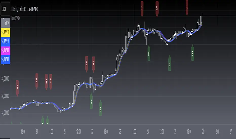
[blackcat] L2 FiboKAMA Adaptive TrendOVERVIEW
The L2 FiboKAMA Adaptive Trend indicator leverages advanced technical analysis techniques by integrating Fibonacci principles with the Kaufman Adaptive Moving Average (KAMA). This combination creates a dynamic and responsive tool designed to adapt seamlessly to changing market conditions. By providing clear buy and sell signals based on adaptive momentum, this indicator helps traders identify potential entry and exit points effectively. Its intuitive design and robust features make it a valuable addition to any trader’s arsenal 📊💹.
According to the principle of Kaufman's Adaptive Moving Average (KAMA), it is a type of moving average line specifically designed for markets with high volatility. Unlike traditional moving averages, KAMA can automatically adjust its period based on market conditions to improve accuracy and responsiveness. This makes it particularly useful for capturing market trends and reducing false signals in varying market environments.
The use of Fibonacci magic numbers (3, 8, 13) enhances the performance and accuracy of KAMA. These numbers have special mathematical properties that align well with the changing trends of KAMA moving averages. Combining them with KAMA can significantly boost its effectiveness, making it a popular choice among traders seeking reliable signals.
This fusion not only smoothens price fluctuations but also ensures quick responses to market changes, offering dependable entry and exit points. Thanks to the flexibility and precision of KAMA combined with Fibonacci magic numbers, traders can better manage risks and aim for higher returns.
FEATURES
Enhanced Kaufman Adaptive Moving Average (KAMA): Incorporates Fibonacci principles for improved adaptability:
Source Price: Allows customization of the price series used for calculation (default: HLCC4).
Fast Length: Determines the period for quicker adjustments to recent price changes.
Slow Length: Sets the period for smoother transitions over longer-term trends.
Dynamic Lines:
KAMA Line: A yellow line representing the primary adaptive moving average, which adapts quickly to new trends.
Trigger Line: A fuchsia line serving as a reference point for detecting crossovers and generating signals.
Visual Cues:
Buy Signals: Green 'B' labels indicating potential buying opportunities.
Sell Signals: Red 'S' labels signaling possible selling points.
Fill Areas: Colored regions between the KAMA and Trigger lines to visually represent trend directions and strength.
Alert Functionality: Generates real-time alerts for both buy and sell signals, ensuring timely notifications for actionable insights 🔔.
Customizable Parameters: Offers flexibility through adjustable inputs, allowing users to tailor the indicator to their specific trading strategies and preferences.
HOW TO USE
Adding the Indicator:
Open your TradingView chart and navigate to the indicators list.
Select L2 FiboKAMA Adaptive Trend and add it to your chart.
Configuring Parameters:
Adjust the Source Price to choose the desired price series (e.g., close, open, high, low).
Set the Fast Length to define how quickly the indicator responds to recent price movements.
Configure the Slow Length to determine the smoothness of long-term trend adaptations.
Interpreting Signals:
Monitor the chart for green 'B' labels indicating buy signals and red 'S' labels for sell signals.
Observe the colored fill areas between the KAMA and Trigger lines to gauge trend strength and direction.
Setting Up Alerts:
Enable alerts within the indicator settings to receive notifications whenever buy or sell signals are triggered.
Customize alert messages and frequencies according to your trading plan.
Combining with Other Tools:
Integrate this indicator with additional technical analysis tools and fundamental research for comprehensive decision-making.
Confirm signals using other indicators like RSI, MACD, or Bollinger Bands for increased reliability.
Optimizing Performance:
Backtest the indicator across various assets and timeframes to understand its behavior under different market conditions.
Fine-tune parameters based on historical performance and current market dynamics.
Integrating Magic Numbers:
Understand the basic principles of KAMA to find suitable entry points for Fibonacci magic numbers.
Utilize the efficiency ratio to measure market volatility and adjust moving average parameters accordingly.
Apply Fibonacci magic numbers (3, 8, 13) to enhance the responsiveness and accuracy of KAMA.
LIMITATIONS
Market Volatility: May produce false signals during periods of extreme volatility or sideways movement.
Parameter Sensitivity: Requires careful tuning of fast and slow lengths to balance responsiveness and stability.
Asset-Specific Behavior: Effectiveness can vary significantly across different financial instruments and time horizons.
Complementary Analysis: Should be used alongside other analytical methods to enhance accuracy and reduce risk.
NOTES
Historical Data: Ensure adequate historical data availability for precise calculations and backtesting.
Demo Testing: Thoroughly test the indicator on demo accounts before deploying it in live trading environments.
Continuous Learning: Stay updated with market trends and continuously refine your strategy incorporating feedback from the indicator's performance.
Risk Management: Always implement proper risk management practices regardless of the signals provided by the indicator.
ADVANCED USAGE TIPS
Multi-Timeframe Analysis: Apply the indicator across multiple timeframes to gain deeper insights into underlying trends.
Divergence Strategy: Look for divergences between price action and the KAMA line to spot potential reversals early.
Volume Integration: Combine volume analysis with the indicator to confirm the strength of identified trends.
Custom Scripting: Modify the script to include additional filters or conditions tailored to your unique trading approach.
IMPROVING KAMA PERFORMANCE
Increase Length: Extend the KAMA length to consider more historical data, reducing the impact of short-term price fluctuations.
Adjust Fast and Slow Lengths: Make KAMA smoother by increasing the fast length and decreasing the slow length.
Use Smoothing Factor: Apply a smoothing factor to control the level of smoothness; typical values range from 0 to 1.
Combine with Other Indicators: Pair KAMA with other smoothing indicators like EMA or SMA for more reliable signals.
Filter Noise: Use filters or other technical analysis tools to eliminate price noise, enhancing KAMA's effectiveness.
Heiken Ashi Supertrend ADXHeiken Ashi Supertrend ADX Indicator
Overview
This indicator combines the power of Heiken Ashi candles, Supertrend indicator, and ADX filter to identify strong trend movements across multiple timeframes. Designed primarily for the cryptocurrency market but adaptable to any tradable asset, this system focuses on capturing momentum in established trends while employing a sophisticated triple-layer stop loss mechanism to protect capital and secure profits.
Strategy Mechanics
Entry Signals
The strategy uses a unique blend of technical signals to identify high-probability trade entries:
Heiken Ashi Candles: Looks specifically for Heiken Ashi candles with minimal or no wicks, which signal strong momentum and trend continuation. These "full-bodied" candles represent periods where price moved decisively in one direction with minimal retracement. These are overlayed onto normal candes for more accuarte signalling and plotting
Supertrend Filter: Confirms the underlying trend direction using the Supertrend indicator (default factor: 3.0, ATR period: 10). Entries are aligned with the prevailing Supertrend direction.
ADX Filter (Optional) : Can be enabled to focus only on stronger trending conditions, filtering out choppy or ranging markets. When enabled, trades only trigger when ADX is above the specified threshold (default: 25).
Exit Signals
Positions are closed when either:
An opposing signal appears (Heiken Ashi candle with no wick in the opposite direction)
Any of the three stop loss mechanisms are triggered
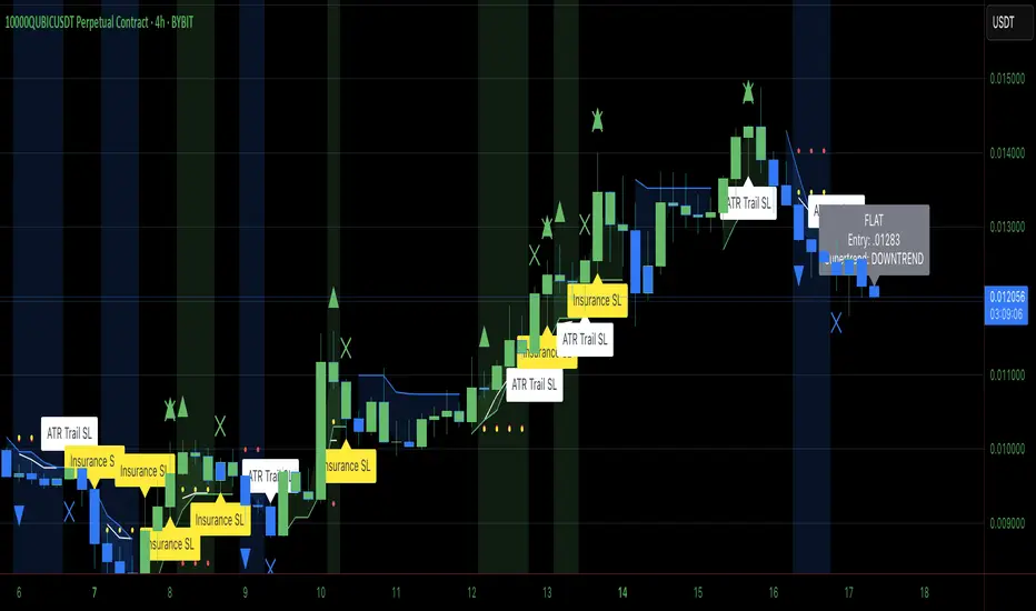
Triple-Layer Stop Loss System
The strategy employs a sophisticated three-tier stop loss approach:
ATR Trailing Stop: Adapts to market volatility and locks in profits as the trend extends. This stop moves in the direction of the trade, capturing profit without exiting too early during normal price fluctuations.
Swing Point Stop: Uses natural market structure (recent highs/lows over a lookback period) to place stops at logical support/resistance levels, honoring the market's own rhythm.
Insurance Stop: A percentage-based safety net that protects against sudden adverse moves immediately after entry. This is particularly valuable when the swing point stop might be positioned too far from entry, providing immediate capital protection.
Optimization Features
Customizable Filters : All components (Supertrend, ADX) can be enabled/disabled to adapt to different market conditions
Adjustable Parameters : Fine-tune ATR periods, Supertrend factors, and ADX thresholds
Flexible Stop Loss Settings : Each of the three stop loss mechanisms can be individually enabled/disabled with customizable parameters
Best Practices for Implementation
[Recommended Timeframes : Works best on 4-hour charts and above, where trends develop more reliably
Market Conditions: Performs well across various market conditions due to the ADX filter's ability to identify meaningful trends
Performance Characteristics
When properly optimized, this has demonstrated profit factors exceeding 3 in backtesting. The approach typically produces generous winners while limiting losses through its multi-layered stop loss system. The ATR trailing stop is particularly effective at capturing extended trends, while the insurance stop provides immediate protection against adverse moves.
The visual components on the chart make it easy to follow the strategy's logic, with position status, entry prices, and current stop levels clearly displayed.
This indicator represents a complete trading system with clearly defined entry and exit rules, adaptive stop loss mechanisms, and built-in risk management through position sizing.
Heiken Ashi Supertrend ADX - StrategyHeiken Ashi Supertrend ADX Strategy
Overview
This strategy combines the power of Heiken Ashi candles, Supertrend indicator, and ADX filter to identify strong trend movements across multiple timeframes. Designed primarily for the cryptocurrency market but adaptable to any tradable asset, this system focuses on capturing momentum in established trends while employing a sophisticated triple-layer stop loss mechanism to protect capital and secure profits.
Strategy Mechanics
Entry Signals
The strategy uses a unique blend of technical signals to identify high-probability trade entries:
Heiken Ashi Candles: Looks specifically for Heiken Ashi candles with minimal or no wicks, which signal strong momentum and trend continuation. These "full-bodied" candles represent periods where price moved decisively in one direction with minimal retracement.
Supertrend Filter : Confirms the underlying trend direction using the Supertrend indicator (default factor: 3.0, ATR period: 10). Entries are aligned with the prevailing Supertrend direction.
ADX Filter (Optional) : Can be enabled to focus only on stronger trending conditions, filtering out choppy or ranging markets. When enabled, trades only trigger when ADX is above the specified threshold (default: 25).
Exit Signals
Positions are closed when either:
An opposing signal appears (Heiken Ashi candle with no wick in the opposite direction)
Any of the three stop loss mechanisms are triggered
Triple-Layer Stop Loss System
The strategy employs a sophisticated three-tier stop loss approach:
ATR Trailing Stop: Adapts to market volatility and locks in profits as the trend extends. This stop moves in the direction of the trade, capturing profit without exiting too early during normal price fluctuations.
Swing Point Stop : Uses natural market structure (recent highs/lows over a lookback period) to place stops at logical support/resistance levels, honoring the market's own rhythm.
Insurance Stop: A percentage-based safety net that protects against sudden adverse moves immediately after entry. This is particularly valuable when the swing point stop might be positioned too far from entry, providing immediate capital protection.
Optimization Features
Customizable Filters: All components (Supertrend, ADX) can be enabled/disabled to adapt to different market conditions
Adjustable Parameters: Fine-tune ATR periods, Supertrend factors, and ADX thresholds
Flexible Stop Loss Settings: Each of the three stop loss mechanisms can be individually enabled/disabled with customizable parameters
Best Practices for Implementation
Recommended Timeframes: Works best on 4-hour charts and above, where trends develop more reliably
Market Conditions: Performs well across various market conditions due to the ADX filter's ability to identify meaningful trends
Position Sizing: The strategy uses a percentage of equity approach (default: 3%) for position sizing
Performance Characteristics
When properly optimized, this strategy has demonstrated profit factors exceeding 3 in backtesting. The approach typically produces generous winners while limiting losses through its multi-layered stop loss system. The ATR trailing stop is particularly effective at capturing extended trends, while the insurance stop provides immediate protection against adverse moves.
The visual components on the chart make it easy to follow the strategy's logic, with position status, entry prices, and current stop levels clearly displayed.
This strategy represents a complete trading system with clearly defined entry and exit rules, adaptive stop loss mechanisms, and built-in risk management through position sizing.

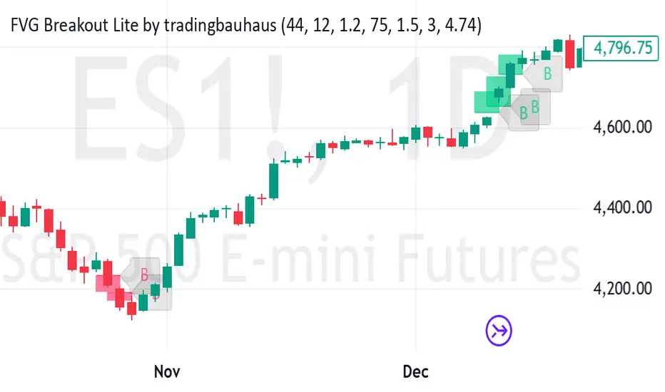
FVG Breakout Lite by tradingbauhausExplanation of "FVG Breakout Lite by tradingbauhaus"
This script is a trading strategy built for TradingView that helps you spot and trade "Fair Value Gaps" (FVGs)—price areas where the market moved quickly, leaving a gap that might act as support or resistance later. It’s designed to catch breakout opportunities when the price moves strongly in one direction, with extra filters to make trades more reliable. Here’s how it works and how you can use it:
What It Does
1. Finds Fair Value Gaps (FVGs):
A "Bullish FVG" happens when the price jumps up quickly, leaving a gap below where it didn’t trade much (e.g., today’s low is higher than the high from two bars ago).
A "Bearish FVG" is the opposite: the price drops fast, leaving a gap above (e.g., today’s high is lower than the low from two bars ago).
The script draws colored boxes on your chart to show these gaps: green for bullish, red for bearish.
2. Spots Breakouts:
It looks for "strong" FVGs by comparing them to a trend (based on the highest highs and lowest lows over a set period).
If a bullish gap forms above the recent highs, or a bearish gap below the recent lows, it’s marked as a breakout opportunity.
3. Adds a Volume Check:
Trades only happen if the market’s volume is higher than usual (e.g., 1.2x the average volume over the last 20 bars). This helps ensure the breakout has real momentum behind it.
4. Trades Automatically:
Long Trades (Buy): If a bullish breakout FVG forms and volume is high, it buys at the current price.
Short Trades (Sell): If a bearish breakout FVG forms with high volume, it sells short.
Each trade comes with a stop loss (to limit losses) and a take profit (to lock in gains), both adjustable by you.
5. Shows Mitigation Lines (Optional):
If you turn on "Display Mitigation Zones," it draws lines at the edge of each breakout FVG. These lines show where the price might return to "fill" the gap later, helping you see key levels.
6. Includes Webull Costs:
The script factors in real trading fees from Webull, like tiny SEC and FINRA fees for selling, and a daily margin cost if you’re borrowing money to trade. These don’t show up on the chart but affect the strategy’s performance in backtesting.
How to Use It
1. Add to Your Chart:
Copy the script into TradingView’s Pine Editor, click "Add to Chart," and it’ll start drawing FVGs and running the strategy.
2. Customize Settings:
Trend Period (Default: 25): How many bars it looks back to define the trend. Longer periods mean fewer but stronger signals.
Volume Lookback (Default: 20) & Volume Threshold (Default: 1.2): Adjust how it measures "high volume." Increase the threshold for stricter trades.
Stop Loss % (Default: 1.5%) & Take Profit % (Default: 3%): Set how much you’re willing to lose or aim to gain per trade.
Margin Rate % (Default: 8.74%): Webull’s rate for borrowing money—lower it if your account qualifies for a better rate.
Display Mitigation Zones (Default: On): Toggle this to see or hide the gap lines.
Colors: Change the green (bullish) and red (bearish) shades to suit your chart.
3. Backtest It:
Go to the "Strategy Tester" tab in TradingView to see how it performs on past data. It’ll show trades, profits, losses, and Webull fees included.
4. Watch It Work:
Green boxes mean bullish FVGs; red boxes mean bearish FVGs. If volume spikes and the price breaks out, you’ll see trades happen automatically.
What to Expect
Visuals: You’ll see colored boxes for FVGs and optional lines showing where they start. These help you spot key price zones even if you’re not trading.
Trades: It’s selective—only trades when FVGs align with a breakout and volume confirms it. Expect fewer trades but with higher potential.
Risk: The stop loss keeps losses in check, while the take profit aims for a 2:1 reward-to-risk ratio by default (3% gain vs. 1.5% loss).
Costs: Webull’s fees are small but baked into the results, so you’re seeing a realistic picture of profits.
Tips for Users
Test it on a small timeframe (like 5-minute charts) for day trading or a larger one (like daily) for swing trading.
Play with the volume threshold—if you get too few trades, lower it (e.g., 1.1); if too many, raise it (e.g., 1.5).
Watch how price reacts to the mitigation lines—they’re often support or resistance zones traders target.
This strategy is lightweight, focused, and built for traders who like breakouts with a bit of confirmation. It’s not foolproof (no strategy is!), but it gives you a clear way to trade FVGs with some smart filters.
Trend Vanguard StrategyHow to Use:
Trend Vanguard Strategy is a multi-feature Pine Script strategy designed to identify market pivots, draw dynamic support/resistance, and generate trade signals via ZigZag breakouts. Here’s how it works and how to use it:
ZigZag Detection & Pivot Points
The script locates significant swing highs and lows using configurable Depth, Deviation, and Backstep values.
It then connects these pivots with lines (ZigZag) to highlight directional changes and prints labels (“Buy,” “Sell,” etc.) at key turning points.
Support & Resistance Trendlines
Pivot highs and lows are used to draw dashed S/R lines in real-time.
When price crosses these lines, the script triggers a breakout signal (long or short).
EMA Overlays
Up to four EMAs (with customizable lengths and colors) can be overlaid on the chart for added trend confirmation.
Enable/disable each EMA independently via the settings.
Repaint Option
Turning on “Smooth Indicator Lines” (repaint) uses future data to refine past pivots.
This can make historical signals look cleaner but does not reflect true historical conditions.
Turning it off ensures signals remain fixed once they appear.
Strategy Entries & Exits
On each new ZigZag “Buy” or “Sell” signal, the script closes any open position and flips to the opposite side (if desired).
Works with the built-in TradingView Strategy engine for backtesting.
Additional Inputs (Placeholders)
Volume Filter and RSI Filter settings exist but are not fully implemented in the current code. Future versions may incorporate these filters more directly.
How to Use
Add to Chart: Click “Indicators” → “Invite-Only Scripts” (or “My Scripts”) and select “Trend Vanguard Strategy.”
Configure Settings:
Adjust ZigZag Depth, Deviation, and Backstep to fine-tune pivot sensitivity.
Enable or disable each EMA to see how it aligns with market trends.
Toggle “Smooth Indicator Lines” on or off depending on whether you want repainting.
Backtest and Forward Test:
Use TradingView’s “Strategy Tester” tab to review hypothetical performance.
Remember that repainting can alter past signals if enabled.
Monitor Live:
Watch for breakout triangles or ZigZag labels to identify potential reversal or breakout trades in real time.
Disclaimer: This script is purely educational and not financial advice. Always combine it with sound risk management and thorough analysis. Enjoy exploring the script, and feel free to experiment with the different settings to match your trading style!

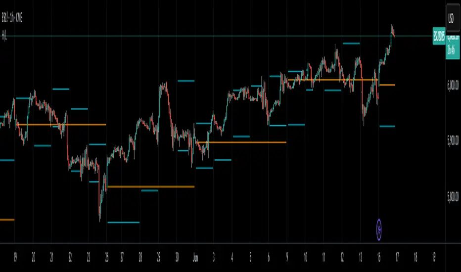
Forward Curve Visualization ToolProvide the spot symbol and the futures product root, and the script automatically scans all relevant contracts for you—no more tedious manual searches. The result is a clean, intuitive chart showing the live forward curve in real time.
It also detects contango or backwardation conditions (based on spot < F1 < F2 < F3).
Future Features:
Plot historical snapshots of the curve (1 day, 1 week, or 1 month ago) to understand market trends over time.
Display additional metrics such as annualized basis, cost of carry (CoC), and even volume or open interest for deeper insights.
If you trade futures and watch the forward curve, this script will give you the actionable data you need and get more ideas or features you’d like to see. Let’s build them together!
Disclaimer
Please remember that past performance may not be indicative of future results.
Due to various factors, including changing market conditions, the strategy may no longer perform as well as in historical backtesting.
This post and the script don’t provide any financial advice.

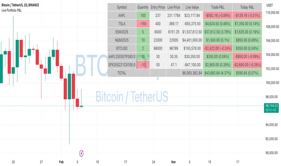
Live Portfolio P<his script calculates live P&L (Profit & Loss) for up to 40 instruments — stocks, ETFs, options, futures, and Forex pairs supported by TradingView. Instead of juggling numerous inputs, you paste your portfolio in CSV format into a single text field, and the script handles the rest. It parses each position and displays a comprehensive table showing the symbol, current price, position value, total P&L, and today’s P&L—all updated in real time.
Key Features
CSV Portfolio Input – Effortlessly import all your positions at once without filling in multiple fields. You can export the position from your broker, save it in the required format, and paste it into this script.
Supports Various Asset Classes – Works with any instrument that TradingView provides data for, including futures, options, and Forex.
Up to 40 Instruments – Track a broad and diverse set of holdings in one place.
Real-Time Updates – Get immediate feedback on live price changes, total value, and current P&L.
Today’s P&L – Monitor your daily performance to gauge short-term trends.
CSV is consumed in the following format:
Symbol (supported TradingView instruments)
Entry Price
Quantity (negative for short position)
Lot Size (for futures/options, it might not be one)
For example:
AAPL,237,100,1
TSLA,400,-150,1
ESM2025,6000,5,50
Planned Enhancements
Multi-Currency Support – Automatically convert and display your positions’ values in different currencies.
Advanced Metrics – Get deeper insights with calculations for drawdown, Sharpe ratio, and more.
Risk Management Tools – Set stop-loss and take-profit levels and receive alerts when thresholds are hit.
Option Greeks & Margin Calculations – Manage complex option strategies and track margin requirements.
Questions for You
What additional features would you like to see?
Are there any specific metrics or analytics you’d find especially valuable?
How might this script fit into your current trading workflow?
Feel free to share your thoughts and suggestions. Your feedback will help shape future updates and make this tool even more helpful for traders like you!
Disclaimer
Please remember that past performance may not be indicative of future results.
Due to various factors, including changing market conditions, the strategy may no longer perform as well as in historical backtesting.
This post and the script don’t provide any financial advice.
Daily COC Strategy with SHERLOCK WAVESThis indicator implements a unique trading strategy known as the "Daily COC (Candle Over Candle) Strategy" enhanced with "SHERLOCK WAVES" for pattern recognition. It's designed for traders looking to capitalize on specific candlestick formations with a negative risk-reward ratio, with the aim of achieving a high win rate (over 70%) through numerous trading opportunities, despite each trade having a higher risk relative to the reward.
Key Features:
Pattern Recognition: Identifies a setup based on three consecutive candles - a red candle followed by a shooting star, then an entry candle that does not break below the shooting star's low.
Negative Risk/Reward Trade Selection: Focuses on entries where the potential stop loss is greater than the take profit, banking on a high win rate to offset the individual trade's negative risk-reward ratio.
Visual Signals:
Green Label: Marks potential entry points at the high of the candle before the entry.
Green Dot: Indicates a winning trade closure.
Red Dot: Signals a losing trade closure.
Blue Circle: Warns when the current candle is within 2% of breaking above the previous candle's high, suggesting a potential setup is developing.
Green Circle: Plots the take profit level.
Red Circle: Plots the stop loss level.
Dynamic Statistics: A live updating label showing the number of trades, wins, losses, open trades, current account balance, and win percentage.
Customizable Parameters:
Risk % per Trade: Adjust the percentage of your account balance you're willing to risk on each trade.
Initial Account Balance: Set your starting balance for tracking performance.
Start Date for Strategy: Define when the strategy should start calculating from, allowing for backtesting.
Alerts:
An alert condition is set for when a potential trade setup is developing, helping traders prepare for entries.
Usage Tips:
This strategy is predicated on the idea that a high win rate can compensate for the negative risk-reward ratio of individual trades. It might not suit all market conditions or traders' risk profiles.
Use this strategy in conjunction with other analysis methods to validate trade setups.
Note: Always backtest thoroughly before applying to live markets. Consider this tool as part of a broader trading strategy, not a standalone solution. Monitor your win rate and adjust your risk management accordingly to ensure the strategy remains profitable over time.
This description now correctly explains the purpose behind the negative risk-reward ratio in the context of your trading strategy.

Statistical Arbitrage Pairs Trading - Long-Side OnlyThis strategy implements a simplified statistical arbitrage (" stat arb ") approach focused on mean reversion between two correlated instruments. It identifies opportunities where the spread between their normalized price series (Z-scores) deviates significantly from historical norms, then executes long-only trades anticipating reversion to the mean.
Key Mechanics:
1. Spread Calculation: The strategy computes Z-scores for both instruments to normalize price movements, then tracks the spread between these Z-scores.
2. Modified Z-Score: Uses a robust measure combining the median and Median Absolute Deviation (MAD) to reduce outlier sensitivity.
3. Entry Signal: A long position is triggered when the spread’s modified Z-score falls below a user-defined threshold (e.g., -1.0), indicating extreme undervaluation of the main instrument relative to its pair.
4. Exit Signal: The position closes automatically when the spread reverts to its historical mean (Z-score ≥ 0).
Risk management:
Trades are sized as a percentage of equity (default: 10%).
Includes commissions and slippage for realistic backtesting.
hector mena Breakout Trading with ATR, RSI and MA CrossTitle: Breakout Trading Strategy with ATR, RSI, and Moving Average Cross
Description (English):
This script combines key technical indicators—ATR (Average True Range), RSI (Relative Strength Index), and Moving Averages—to provide a comprehensive breakout trading strategy. It is designed to help traders identify significant breakout levels and confirm signals with momentum and trend analysis.
How It Works:
ATR for Breakout Levels:
The ATR is used to calculate dynamic breakout levels by adjusting the highest resistance and lowest support levels with a customizable multiplier. This ensures that breakout levels adapt to market volatility.
RSI for Momentum Confirmation:
The RSI identifies overbought and oversold conditions, providing an additional layer of confirmation for breakouts. A breakout accompanied by an RSI signal can indicate stronger momentum.
Moving Average Cross for Trend Validation:
Two simple moving averages (short-term and long-term) are included to validate the trend. A crossover suggests a potential change in trend, aligning with breakout signals.
Why Combine These Indicators?
The ATR ensures breakout levels are realistic and volatility-adjusted.
The RSI avoids false signals by confirming if the price has momentum during a breakout.
Moving Average crossovers add trend-following confirmation, helping traders align with market direction.
The combination provides a robust framework to filter out false signals and improve the reliability of trading decisions.
Key Features:
Breakout Levels: Upper and lower breakout levels dynamically calculated using ATR.
RSI Confirmation: Visual overbought (70) and oversold (30) levels and RSI plot.
Trend Validation: Short and long-term moving averages plotted on the chart with crossover signals.
Visual Alerts: Clear "BUY" and "SELL" labels for actionable signals.
Custom Alerts: Configurable alerts for breakouts and moving average crossovers.
How to Use It:
Adjust the parameters (ATR length, multiplier, RSI length, and moving averages) based on your trading strategy.
Look for "BUY" signals when:
Price breaks above the resistance level, and RSI indicates oversold conditions.
Moving averages cross bullishly.
Look for "SELL" signals when:
Price breaks below the support level, and RSI indicates overbought conditions.
Moving averages cross bearishly.
Use alerts for automated notifications about potential trades.
Notes:
This script is intended for educational purposes. Use it alongside proper risk management techniques and backtesting.
Always test in demo mode before applying it to live trading.

[blackcat] L2 Waveband Trading█ OVERVIEW
The Waveband Trading script calculates trading signals based on a modified Relative Strength Index (RSI)-like system combined with specific price action criteria. It plots two lines representing different smoothed RSI-like indicators and marks potential buying opportunities labeled as "S" for stronger trends and "B" for weaker but still favorable ones.
█ LOGICAL FRAMEWORK
The script begins by defining the waveband_trading_signals function which computes RSI-like metrics and determines buy signals under certain conditions. The main sections include input parameter definitions, function calls, data processing within the function, and plot commands for visual representation. Data flows from historical OHLCV data to various technical computations like EMAs and SMAs before being evaluated against user-defined thresholds to generate trade signals.
█ CUSTOM FUNCTIONS
Waveband Trading Signals:
• Purpose: Computes waveband trading signals using a customized version of the RSI indicator.
• Parameters:
— overboughtLevel: Threshold level indicating market overbought condition.
— oversoldLevel: Threshold level indicating market oversold condition.
— strongHoldLevel: Strong hold condition threshold between neutral and overbought states.
— moderateHoldLevel: Moderate hold condition threshold below strong hold level.
• [b>Returns: A tuple containing:
— k: Smoothed RSI-like metric.
— d: Further smoothed version of 'k'.
— buySignalStrong: Boolean indicating a strong trend buy signal.
— buySignalWeak: Boolean indicating a weak but promising buy signal.
█ KEY POINTS AND TECHNIQUES
• Utilizes EMA and SMA functions to smooth out price variations effectively.
• Employs crossover logic between fast ('k') and slow ('d') indicators to identify entry points.
• Incorporates volume checks ensuring increasing interest in trades aligns with upwards momentum.
• Leverages predefined threshold levels allowing flexibility to adapt to varying market conditions.
• Uses the new labeling feature ( label.new ) introduced in Pine Script v5 for marking significant chart events visually.
█ EXTENDED KNOWLEDGE AND APPLICATIONS
Potential enhancements could involve incorporating additional filters such as MACD crossovers or Fibonacci retracement levels alongside optimizing current conditions via backtesting. This technique might also prove useful in other strategies requiring robust confirmation methods beyond simple price action; alternatively, adapting it into a more automated form for execution on exchanges offering API access. Understanding key functionalities like relative strength assessment, smoothed averaging techniques, and conditional buy/sell rules enriches one’s toolkit when developing complex trading algorithms tailored specifically toward personal investment philosophies.

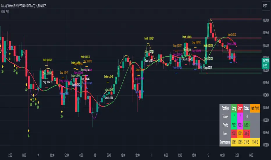
HMA Buy Sell Signals - Profit ManagerNote : Settings should be adjusted according to the selected time frame. Try to find the best setting according to the profitability rate
Overall Functionality
This script combines several trading tools to create a comprehensive system for trend analysis, trade execution, and performance tracking. Users can identify market trends using specific moving averages and RSI indicators while managing profit and loss levels automatically.
Trend Detection and Trade Signals
Hull Moving Averages (HMA):
Two HMAs (a faster one and a slower one) are used to determine the market trend.
A buy signal is generated when the faster HMA crosses above the slower HMA.
Conversely, a sell signal is triggered when the faster HMA crosses below the slower one.
Visual Feedback:
Trend lines on the chart change color to reflect the trend direction (e.g., green for upward trends and red for downward trends).
Trade Levels and Management
Entry, Take-Profit, and Stop-Loss Levels:
When the trend shifts upwards, the script calculates entry, take-profit, and stop-loss levels based on the opening price.
Similarly, for downward trends, these levels are determined for short trades.
Commission Tracking:
Each trade includes a commission cost, which is factored into net profit and loss calculations.
Dynamic Labels:
Entry, take-profit, and stop-loss levels are visually marked on the chart for easier tracking.
Performance Tracking
Profit and Loss Tracking:
The script keeps a running total of profits, losses, and commissions for both long and short trades.
It also calculates the net profit after all costs are considered.
Performance Table:
A table is displayed on the chart summarizing:
The number of trades.
Total profit and loss for long and short positions.
Commission costs.
Net profit.
Fractal Support and Resistance
Dynamic Lines:
The script identifies the most recent significant highs and lows using fractals.
It draws support and resistance lines that automatically update as new fractals form.
Simplified Visuals:
The chart always shows the last two support and resistance lines, keeping the visualization clean and focused.
RSI-Based Signals
Overbought and Oversold Levels:
RSI is used to identify overbought (above 80) and oversold (below 20) conditions.
The script generates buy signals at oversold levels and sell signals at overbought levels.
Chart Indicators:
Arrows and labels appear on the chart to highlight these RSI-based opportunities.
Customization
The script allows users to customize key parameters such as:
Moving average lengths for trend detection.
Take-profit and stop-loss percentages.
Timeframes for backtesting.
Starting capital and commission rates.
Conclusion
This script is a versatile tool for traders, combining trend detection, automated trade management, and visual feedback. It simplifies decision-making by providing clear signals and tracking performance metrics, making it suitable for both beginners and experienced traders.
* The most recently drawn fractals represent potential support and resistance levels. If the price aligns with these levels at the time of entering a trade, it may indicate a likelihood of reversal. In such cases, it’s advisable to either avoid entering the trade altogether or proceed with increased caution.
Custom Strategy: ETH Martingale 2.0Strategic characteristics
ETH Little Martin 2.0 is a self-developed trading strategy based on the Martingale strategy, mainly used for trading ETH (Ethereum). The core idea of this strategy is to place orders in the same direction at a fixed price interval, and then use Martin's multiple investment principle to reduce losses, but this is also the main source of losses.
Parameter description:
1 Interval: The minimum spacing for taking profit, stop loss, and opening/closing of orders. Different targets have different spacing. Taking ETH as an example, it is generally recommended to have a spacing of 2% for fluctuations in the target.
2 Base Price: This is the price at which you triggered the first order. Similarly, I am using ETH as an example. If you have other targets, I suggest using the initial value of a price that can be backtesting. The Base Price is only an initial order price and has no impact on subsequent orders.
3 Initial Order Amount: Users can set an initial order amount to control the risk of each transaction. If the stop loss is reached, we will double the amount based on this value. This refers to the value of the position held, not the number of positions held.
4 Loss Multiplier: The strategy will increase the next order amount based on the set multiple after the stop loss, in order to make up for the previous losses through a larger position. Note that after taking profit, it will be reset to 1 times the Initial Order Amount.
5. Long Short Operation: The first order of the strategy is a multiple entry, and in subsequent orders, if the stop loss is reached, a reverse order will be opened. The position value of a one-way order is based on the Loss Multiplier multiple investment, so it is generally recommended that the Loss Multiplier default to 2.
Improvement direction
Although this strategy already has a certain trading logic, there are still some improvement directions that can be considered:
1. Dynamic adjustment of spacing: Currently, the spacing is fixed, and it can be considered to dynamically adjust the spacing based on market volatility to improve the adaptability of the strategy. Try using dynamic spacing, which may be more suitable for the actual market situation.
2. Filtering criteria: Orders and no orders can be optimized separately. The biggest problem with this strategy is that it will result in continuous losses during fluctuations, and eventually increase the investment amount. You can consider filtering out some fluctuations or only focusing on trend trends.
3. Risk management: Add more risk management measures, such as setting a maximum loss limit to avoid huge losses caused by continuous stop loss.
4. Optimize the stop loss multiple: Currently, the stop loss multiple is fixed, and it can be considered to dynamically adjust the multiple according to market conditions to reduce risk.

Enhanced Reversal DetectorEnhanced Reversal Detector - Script Description
Overview:
The Enhanced Reversal Detector is a highly refined indicator designed to identify precise trend reversals in financial markets. It improves upon the original reversal detection logic by incorporating additional filters for trend confirmation (using EMA), volume spikes, and candle patterns. These enhancements significantly increase the reliability and accuracy of reversal signals, making it an excellent tool for both short-term and long-term traders.
Key Features
Candle Lookback Logic:
The indicator evaluates historical price action over a user-defined lookback period to detect potential reversal zones.
Bullish reversal conditions are met when price consistently tests lows, and bearish reversal conditions are met when price tests highs.
Trend Confirmation (EMA Filter):
To ensure that reversal signals align with the broader market trend, the indicator incorporates an Exponential Moving Average (EMA) filter.
Bullish signals are only triggered when the price is above the EMA, while bearish signals are only triggered when the price is below the EMA.
Volume Spike Filter:
The indicator checks for significant increases in trading volume to confirm that the reversal is supported by strong market activity.
Volume spikes are calculated as trading volume exceeding a multiple of the 20-bar average volume (default: 1.5x).
Confirmation Period:
Users can define a confirmation window within which reversal signals must be validated.
This reduces false positives and ensures only strong reversals are considered.
Non-Repainting Mode:
Offers a non-repainting option, where signals are based on confirmed conditions from previous bars, ensuring reliability for backtesting.
Visual and Alert Features:
Clear visual markers on the chart indicate bullish (green triangle) and bearish (red triangle) reversal points.
Alert notifications can be enabled for both bullish and bearish reversals, keeping traders informed in real-time.
Inputs
Candle Lookback: Number of candles to evaluate for reversal conditions.
Confirm Within: Number of candles within which a reversal must be validated.
Non-Repainting Mode: Option to enable or disable repainting for signals.
EMA Length: The length of the Exponential Moving Average used for trend confirmation.
Volume Spike Multiplier: Multiplier for identifying significant increases in trading volume.
How It Works
Reversal Detection:
Bullish signals are triggered when:
Price consistently tests recent lows (lookback period).
Price closes above the EMA.
A significant volume spike occurs.
Bearish signals are triggered under opposite conditions (price testing highs, closing below EMA, and volume spike).
Signal Filtering:
Incorporates EMA and volume-based filters to eliminate false positives and focus on high-confidence reversal signals.
Alert Notifications:
Alerts notify users of bullish or bearish reversal opportunities as soon as they are detected.
Use Cases
Scalping and Day Trading:
Ideal for identifying reversals on lower timeframes (e.g., 1-minute or 5-minute charts).
Swing Trading:
Works effectively on higher timeframes (e.g., 1-hour or daily charts) for capturing significant
trend reversals.
Volatile Markets:
Particularly useful in high-volatility markets like cryptocurrencies or forex.
Customization Tips
Adjust the lookback period to fine-tune the sensitivity of the reversal detection.
Increase the volume spike multiplier for markets with irregular trading volumes to focus on significant moves.
Experiment with the EMA length to align signals with your trading strategy's preferred trend duration.
Conclusion
The Enhanced Reversal Detector combines advanced price action analysis, trend confirmation, and market participation filters to deliver high-accuracy reversal signals. With its customizable settings and robust filtering mechanisms, this indicator is an invaluable tool for identifying profitable trading opportunities while minimizing noise and false signals.
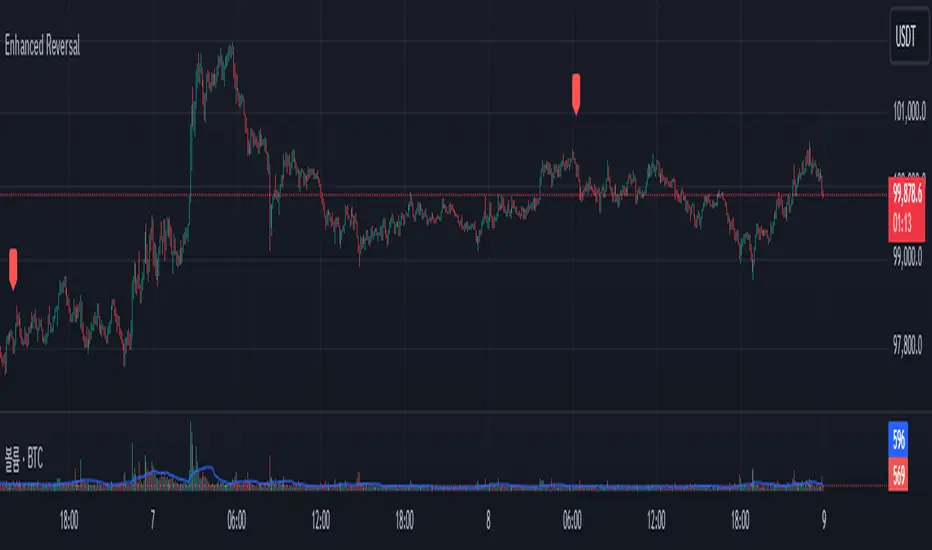
Fibonacci ATR Fusion - Strategy [presentTrading]Open-script again! This time is also an ATR-related strategy. Enjoy! :)
If you have any questions, let me know, and I'll help make this as effective as possible.
█ Introduction and How It Is Different
The Fibonacci ATR Fusion Strategy is an advanced trading approach that uniquely integrates Fibonacci-based weighted averages with the Average True Range (ATR) to identify and capitalize on significant market trends.
Unlike traditional strategies that rely on single indicators or static parameters, this method combines multiple timeframes and dynamic volatility measurements to enhance precision and adaptability. Additionally, it features a 4-step Take Profit (TP) mechanism, allowing for systematic profit-taking at various levels, which optimizes both risk management and return potential in long and short market positions.
BTCUSD 6hr Performance
█ Strategy, How It Works: Detailed Explanation
The Fibonacci ATR Fusion Strategy utilizes a combination of technical indicators and weighted averages to determine optimal entry and exit points. Below is a breakdown of its key components and operational logic.
🔶 1. Enhanced True Range Calculation
The strategy begins by calculating the True Range (TR) to measure market volatility accurately.
TR = max(High - Low, abs(High - Previous Close), abs(Low - Previous Close))
High and Low: Highest and lowest prices of the current trading period.
Previous Close: Closing price of the preceding trading period.
max: Selects the largest value among the three calculations to account for gaps and limit movements.
🔶 2. Buying Pressure (BP) Calculation
Buying Pressure (BP) quantifies the extent to which buyers are driving the price upwards within a period.
BP = Close - True Low
Close: Current period's closing price.
True Low: The lower boundary determined in the True Range calculation.
🔶 3. Ratio Calculation for Different Periods
To assess the strength of buying pressure relative to volatility, the strategy calculates a ratio over various Fibonacci-based timeframes.
Ratio = 100 * (Sum of BP over n periods) / (Sum of TR over n periods)
n: Length of the period (e.g., 8, 13, 21, 34, 55).
Sum of BP: Cumulative Buying Pressure over n periods.
Sum of TR: Cumulative True Range over n periods.
This ratio normalizes buying pressure, making it comparable across different timeframes.
🔶 4. Weighted Average Calculation
The strategy employs a weighted average of ratios from multiple Fibonacci-based periods to smooth out signals and enhance trend detection.
Weighted Avg = (w1 * Ratio_p1 + w2 * Ratio_p2 + w3 * Ratio_p3 + w4 * Ratio_p4 + Ratio_p5) / (w1 + w2 + w3 + w4 + 1)
w1, w2, w3, w4: Weights assigned to each ratio period.
Ratio_p1 to Ratio_p5: Ratios calculated for periods p1 to p5 (e.g., 8, 13, 21, 34, 55).
This weighted approach emphasizes shorter periods more heavily, capturing recent market dynamics while still considering longer-term trends.
🔶 5. Simple Moving Average (SMA) of Weighted Average
To further smooth the weighted average and reduce noise, a Simple Moving Average (SMA) is applied.
Weighted Avg SMA = SMA(Weighted Avg, m)
- m: SMA period (e.g., 3).
This smoothed line serves as the primary signal generator for trade entries and exits.
🔶 6. Trading Condition Thresholds
The strategy defines specific threshold values to determine optimal entry and exit points based on crossovers and crossunders of the SMA.
Long Condition = Crossover(Weighted Avg SMA, Long Entry Threshold)
Short Condition = Crossunder(Weighted Avg SMA, Short Entry Threshold)
Long Exit = Crossunder(Weighted Avg SMA, Long Exit Threshold)
Short Exit = Crossover(Weighted Avg SMA, Short Exit Threshold)
Long Entry Threshold (T_LE): Level at which a long position is triggered.
Short Entry Threshold (T_SE): Level at which a short position is triggered.
Long Exit Threshold (T_LX): Level at which a long position is exited.
Short Exit Threshold (T_SX): Level at which a short position is exited.
These conditions ensure that trades are only executed when clear trends are identified, enhancing the strategy's reliability.
Previous local performance
🔶 7. ATR-Based Take Profit Mechanism
When enabled, the strategy employs a 4-step Take Profit system to systematically secure profits as the trade moves in the desired direction.
TP Price_1 Long = Entry Price + (TP1ATR * ATR Value)
TP Price_2 Long = Entry Price + (TP2ATR * ATR Value)
TP Price_3 Long = Entry Price + (TP3ATR * ATR Value)
TP Price_1 Short = Entry Price - (TP1ATR * ATR Value)
TP Price_2 Short = Entry Price - (TP2ATR * ATR Value)
TP Price_3 Short = Entry Price - (TP3ATR * ATR Value)
- ATR Value: Calculated using ATR over a specified period (e.g., 14).
- TPxATR: User-defined multipliers for each take profit level.
- TPx_percent: Percentage of the position to exit at each TP level.
This multi-tiered exit strategy allows for partial position closures, optimizing profit capture while maintaining exposure to potential further gains.
█ Trade Direction
The Fibonacci ATR Fusion Strategy is designed to operate in both long and short market conditions, providing flexibility to traders in varying market environments.
Long Trades: Initiated when the SMA of the weighted average crosses above the Long Entry Threshold (T_LE), indicating strong upward momentum.
Short Trades: Initiated when the SMA of the weighted average crosses below the Short Entry Threshold (T_SE), signaling robust downward momentum.
Additionally, the strategy can be configured to trade exclusively in one direction—Long, Short, or Both—based on the trader’s preference and market analysis.
█ Usage
Implementing the Fibonacci ATR Fusion Strategy involves several steps to ensure it aligns with your trading objectives and market conditions.
1. Configure Strategy Parameters:
- Trading Direction: Choose between Long, Short, or Both based on your market outlook.
- Trading Condition Thresholds: Set the Long Entry, Short Entry, Long Exit, and Short Exit thresholds to define when to enter and exit trades.
2. Set Take Profit Levels (if enabled):
- ATR Multipliers: Define how many ATRs away from the entry price each take profit level is set.
- Take Profit Percentages: Allocate what percentage of the position to close at each TP level.
3. Apply to Desired Chart:
- Add the strategy to the chart of the asset you wish to trade.
- Observe the plotted Fibonacci ATR and SMA Fibonacci ATR indicators for visual confirmation.
4. Monitor and Adjust:
- Regularly review the strategy’s performance through backtesting.
- Adjust the input parameters based on historical performance and changing market dynamics.
5. Risk Management:
- Ensure that the sum of take profit percentages does not exceed 100% to avoid over-closing positions.
- Utilize the ATR-based TP levels to adapt to varying market volatilities, maintaining a balanced risk-reward ratio.
█ Default Settings
Understanding the default settings is crucial for optimizing the Fibonacci ATR Fusion Strategy's performance. Here's a precise and simple overview of the key parameters and their effects:
🔶 Key Parameters and Their Effects
1. Trading Direction (`tradingDirection`)
- Default: Both
- Effect: Determines whether the strategy takes both long and short positions or restricts to one direction. Selecting Both allows maximum flexibility, while Long or Short can be used for directional bias.
2. Trading Condition Thresholds
Long Entry (long_entry_threshold = 58.0): Higher values reduce false positives but may miss trades.
Short Entry (short_entry_threshold = 42.0): Lower values capture early short trends but may increase false signals.
Long Exit (long_exit_threshold = 42.0): Exits long positions early, securing profits but potentially cutting trends short.
Short Exit (short_exit_threshold = 58.0): Delays short exits to capture favorable movements, avoiding premature exits.
3. Take Profit Configuration (`useTakeProfit` = false)
- Effect: When enabled, the strategy employs a 4-step TP mechanism to secure profits at multiple levels. By default, it is disabled to allow users to opt-in based on their trading style.
4. ATR-Based Take Profit Multipliers
TP1 (tp1ATR = 3.0): Sets the first TP at 3 ATRs for initial profit capture.
TP2 (tp2ATR = 8.0): Targets larger trends, though less likely to be reached.
TP3 (tp3ATR = 14.0): Optimizes for extreme price moves, seldom triggered.
5. Take Profit Percentages
TP Level 1 (tp1_percent = 12%): Secures 12% at the first TP.
TP Level 2 (tp2_percent = 12%): Exits another 12% at the second TP.
TP Level 3 (tp3_percent = 12%): Closes an additional 12% at the third TP.
6. Weighted Average Parameters
Ratio Periods: Fibonacci-based intervals (8, 13, 21, 34, 55) balance responsiveness.
Weights: Emphasizes recent data for timely responses to market trends.
SMA Period (weighted_avg_sma_period = 3): Smoothens data with minimal lag, balancing noise reduction and responsiveness.
7. ATR Period (`atrPeriod` = 14)
Effect: Sets the ATR calculation length, impacting TP sensitivity to volatility.
🔶 Impact on Performance
- Sensitivity and Responsiveness:
- Shorter Ratio Periods and Higher Weights: Make the weighted average more responsive to recent price changes, allowing quicker trade entries and exits but increasing the likelihood of false signals.
- Longer Ratio Periods and Lower Weights: Provide smoother signals with fewer false positives but may delay trade entries, potentially missing out on significant price moves.
- Profit Taking:
- ATR Multipliers: Higher multipliers set take profit levels further away, targeting larger price movements but reducing the probability of reaching these levels.
- Fixed Percentages: Allocating equal percentages at each TP level ensures consistent profit realization and risk management, preventing overexposure.
- Trade Direction Control:
- Selecting Specific Directions: Restricting trades to Long or Short can align the strategy with market trends or personal biases, potentially enhancing performance in trending markets.
- Risk Management:
- Take Profit Percentages: Dividing the position into smaller percentages at multiple TP levels helps lock in profits progressively, reducing risk and allowing the remaining position to ride further trends.
- Market Adaptability:
- Weighted Averages and ATR: By combining multiple timeframes and adjusting to volatility, the strategy adapts to different market conditions, maintaining effectiveness across various asset classes and timeframes.
---
If you want to know more about ATR, can also check "SuperATR 7-Step Profit".
Enjoy trading.