Quadratic Least Squares Moving Average - Smoothing + Forecast Introduction
Technical analysis make often uses of classical statistical procedures, one of them being regression analysis, and since fitting polynomial functions that minimize the sum of squares can be achieved with the use of the mean, variance, covariance...etc, technical analyst only needed to replace the mean in all those calculations with a moving average, we then end up with a low lag filter called least squares moving average (lsma) .
The least squares moving average could be classified as a rolling linear regression, altho this sound really bad it is useful to understand the relationship of both methods, both have the same form, that is ax + b , where a and b are coefficients of the model. However in a simple linear regression a and b are constant, while the lsma use variables instead.
In a simple lsma we model the relationship of the closing price (dependent variable) with a linear sequence (independent variable), therefore x = 1,2,3,4..etc. However we can use polynomial of higher degrees to model such relationship, this is required if we want more reactivity. Therefore we can use a quadratic form, that is ax^2 + bx + c , where a,b and c are variables.
This is the quadratic least squares moving average (qlsma), a not so official term, but we'll stick with it because it still represent the aim of the filter quite well. In this indicator i make the calculations of the qlsma less troublesome, therefore one might understand how it would work, note that in general the coefficients of a polynomial regression model are found using matrix calculus.
The Indicator
A qlsma, unlike the classic lsma, will fit better to the price and will be more reactive, this is the advantage of using an higher degrees for its calculation, we can model more complex relationship.
lsma in green, qlsma in red, with both length = 200
However the over/under shoots are greater, i'll explain why in the next sections, but this is one of the drawbacks of using higher degrees.
The indicator allow to forecast future values, the ahead period of the forecast is determined by the forecast setting. The value for this setting should be lower than length, else the forecasts can easily over/under shoot which heavily damage the forecast. In order to get a view on how well the forecast is performing you can check the option "Show past predicted values".
Of course understanding the logic behind the forecast is important, in short regressions models best fit a certain curve to the data, this curve can be a line (linear regression), a parabola (quadratic regression) and so on, the type of curve is determined by the degree of the polynomial used, here 2, which is a parabola. Lets use a linear regression model as example :
ax + b where x is a linear sequence 1,2,3...and a/b are constants. Our goal is to find the values for a and b that minimize the sum of squares of the line with the dependent variable y, here the closing price, so our hypothesis is that :
closing price = ax + b + ε
where ε is white noise, a component that the model couldn't forecast. The forecast of the closing price 14 step ahead would be equal to :
closing price 14 step aheads = a(x+14) + b
Since x is a linear sequence we only need to sum it with the forecasting horizon period, the same is done here with :
a*(n+forecast)^2 + b*(n + forecast) + c
Note that the forecast proposed in the indicator is more for teaching purpose that anything else, this indicator can't possibly forecast future values, even on a meh rate.
Low lag filters have been used to provide noise free crosses with slow moving average, a bad practice in my opinion due to the ability low lag filters have to overshoot/undershoot, more interesting use cases might be to use the qlsma as input for other indicators.
On The Code
Some of you might know that i posted a "quadratic regression" indicator long ago, the original calculations was coming from a forum, but because the calculation was ugly as hell as well as extra inefficient (dogfood level) i had to do something about it, the name was also terribly misleading.
We can see in the code that we make heavy use of the variance and covariance, both estimated with :
VAR(x) = SMA(x^2) - SMA(x)^2
COV(x,y) = SMA(xy) - SMA(x)SMA(y)
Those elements are then combined, we can easily recognize the intercept element c , who don't change much from the classical lsma.
As Digital Filter
The frequency response of the qlsma is similar to the one of the lsma, those filters amplify certain frequencies in the passband, and have ripples in the stop band. There is something interesting about those filters, first using higher degrees allow to greater boost of the frequencies in the passband, which result in greater over/under shoots. Another funny thing is that the peak/valley of the ripples is equal the peak or valley in the ripples of another lsma of different degree.
The transient response of those filters, that is impulse response, step response...etc is related to the degree of the polynomial used, therefore lets denote a lsma of degree p : lsma(p) , the impulse response of lsma(p) is a polynomial of degree p, and the step response is simple a polynomial of order p+1.
This is why it was more interesting to estimate the qlsma using convolution, however we can no longer forecast future values.
Conclusion
I proposed a more usable quadratic least squares moving average, with more options, as well as a cleaner and more efficient code. The process of shrinking the original code is made easier when you know about the estimations of both variance and covariance.
I hope the proposed indicator/calculation is useful.
Thx for reading !
Pesquisar nos scripts por "VAR+计量模型+黄金期货"

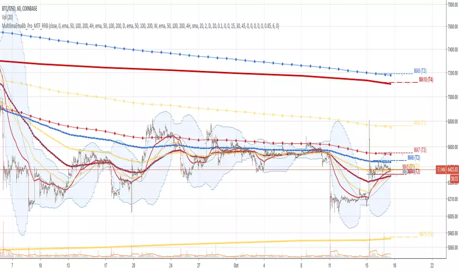
Multi SMA EMA WMA HMA BB (4x3 MAs Bollinger Bands) Pro MTF - RRBMulti SMA EMA WMA HMA 4x3 Moving Averages with Bollinger Bands Pro MTF by RagingRocketBull 2018
Version 1.0
This indicator shows multiple MAs of any type SMA EMA WMA HMA etc with BB and MTF support, can show MAs as dynamically moving levels.
There are 4 MA groups + 1 BB group. You can assign any type/timeframe combo to a group, for example:
- EMAs 50,100,200 x H1, H4, D1, W1 (4 TFs x 3 MAs x 1 type)
- EMAs 8,13,21,55,100,200 x M15, H1 (2 TFs x 6 MAs x 1 type)
- D1 EMAs and SMAs 12,26,50,100,200,400 (1 TF x 6 MAs x 2 types)
- H1 WMAs 7,77,231; H4 HMAs 50,100,200; D1 EMAs 144,169,233; W1 SMAs 50,100,200 (4 TFs x 3 MAs x 4 types)
- +1 extra MA type/timeframe for BB
compile time: 25-30 sec
full redraw time after parameter change in UI: 3 sec
There are several versions: Simple, MTF, Pro MTF, Advanced MTF and Ultimate MTF. This is the Pro MTF version. The Differences are listed below. All versions have BB
- Simple: you have 2 groups of MAs that can be assigned any type (5+5)
- MTF: +2 custom Timeframes for each group (2x5 MTF)
- Pro MTF: +4 custom Timeframes for each group (4x3 MTF), MA levels and show max bars back options
- Advanced MTF: +2 extra MAs/group (4x5 MTF), custom Ticker/Symbol, backreferences for type, TF and MA lengths in UI
- Ultimate MTF: +individual settings for each MA, custom Ticker/Symbols
Features:
- 4x3 = 12 MAs of any type including Hull Moving Average (HMA)
- 4x MTF groups with step line smoothing
- BB +1 extra TF/type for BB MAs
- 12 MA levels with adjustable group offsets, indents and shift
- show max bars back
- you can show/hide both groups of MAs/levels and individual MAs
Notes:
1. based on 3EmaBB, uses plot*, barssince and security functions
2. you can't set certain constants from input due to Pinescript limitations - change the code as needed, recompile and use as a private version
3. Levels = trackprice implementation
4. Show Max Bars Back = show_last implementation
5. uses timeframe textbox instead of input resolution to allow for 120 240 and other custom TFs. Also supports TFs in hours: 2H or H2
6. swma has a fixed length = 4, alma and linreg have additional offset and smoothing params
7. Smoothing is applied by default for visual aesthetics on MTF. To use exact ma mtf values (lines with stair stepping) - disable it
MTF Notes:
- uses simple timeframe textbox instead of input resolution dropdown to allow for 120, 240 and other custom TFs, also supports timeframes in H: 2H, H2
- Groups that are not assigned a Custom TF will use Current Timeframe (0).
- MTF will work for any MA type assigned to the group
- MTF works both ways: you can display a higher TF MA/BB on a lower TF or a lower TF MA/BB on a higher TF.
- MTF MA values are normally aligned at the boundary of their native timeframe. This produces stair stepping when a higher TF MA is viewed on a lower TF.
Therefore X Y Point Density/Smoothing is applied by default on MA MTF for visual aesthetics. Set both to 0 to disable and see exact ma mtf values (lines with stair stepping and original mtf alignment).
- Smoothing is disabled for BB MTF bands because fill doesn't work with smoothed MAs after duplicate values are replaced with na.
- MTF MA Value fluctuation is possible on the current bar due to default security lookahead
Smoothing:
- X,Y == 0 - X,Y smoothing disabled (stair stepping on high TFs)
- X == 0, Y > 0 - X,Y smoothing applied to all TFs
- Y == 0, X > 0 - X smoothing applied to all TFs < deltaX_max_tf, Y smoothing disabled
- X > 0, Y > 0 - Y smoothing applied to all TFs, then X smoothing applied to all TFs < deltaX_max_tf
X Smoothing with Y == 0 - shows only every deltaX-th point starting from the first bar.
X Smoothing with Y > 0 - shows only every deltaX-th point starting from the last shown Y point, essentially filling huge gaps remaining after Y Smoothing with points and preserving the curve's general shape
X Smoothing on high TFs with already scarce points produces weird curve shapes, it works best only on high density lower TFs
Y Smoothing reduces points on all TFs, removes adjacent points with prices within deltaY, while preserving the smaller curve details.
A combination of X,Y produces the most accurate smoothing. Higher delta value - larger range, more points removed.
Show Max Bars Back:
- can't set plot show_last from input -> implemented using a timenow based range check
- you can't delete/modify history once plotted, so essentially it just sets a start point for plotting (from num_bars bars back) that works only in realtime mode (not in replay)
Levels:
You can plot current MA value using plot trackprice=true or by checking Show Price Line in Style. Problem is:
- you can only change color (not the dashed line style, width), have both ma + price line (not just the line), and it's full screen wide
- you can't set plot trackprice from input => implemented using plotshape/plotchar with fixed text labels serving as levels
- there's no other way of creating a dynamic level: hline, plot, offset - nothing else works.
- you can't plot a text var - all text strings must be constants, so you can't change the style, width and text labels without recompiling.
- from input you can only adjust offset, indent and shift for each level group, and change color
- the dot below each level line is the exact MA value. If you want just the line swap plotshape with plotchar, recompile and save as your private version, adjust Y shift.
To speed up redraw times: reduce last_bars to ~2000, recompile and use as your own private version
Pinescript is a rudimentary language (should be called Painscript instead) that can basically only plot data. You can't do much else. Please see the code for tips and hints.
Certain things just can't be done or require shady workarounds and weeks of testing trying to resolve weird node.js compiler errors.
Feel free to learn from/reuse/change the code as needed and use as your own private version. See comments in code. Good Luck!
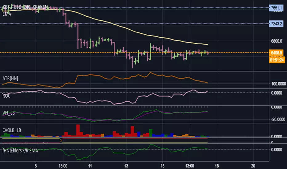
Ehlers Forward Reverse EMAThis is Ehlers most recent indicator, today is 6/17/18 "Forward and Reverse EMA". I have done my best to translate the code form trade stations easy language.
If anyone knows easy language could they check my translation against the easy language code below.
{
Forward / Reverse EMA
(c) 2017 John F. Ehlers
}
Inputs:
AA(.1);
Vars:
CC(.9),
RE1(0),
RE2(0),
RE3(0),
RE4(0),
RE5(0),
RE6(0),
RE7(0),
RE8(0),
EMA(0),
Signal(0);
CC = 1 - AA;
EMA = AA*Close + CC*EMA ;
RE1 = CC*EMA + EMA ;
RE2 = Power(CC, 2)*RE1 + RE1 ;
RE3 = Power(CC, 4)*RE2 + RE2 ;
RE4 = Power(CC, 8)*RE3 + RE3 ;
RE5 = Power(CC, 16)*RE4 + RE4 ;
RE6 = Power(CC, 32)*RE5 + RE5 ;
RE7 = Power(CC, 64)*RE6 + RE6 ;
RE8 = Power(CC, 128)*RE7 + RE7 ;
Signal = EMA - AA*RE8;
Plot1(Signal);
Plot2(0);
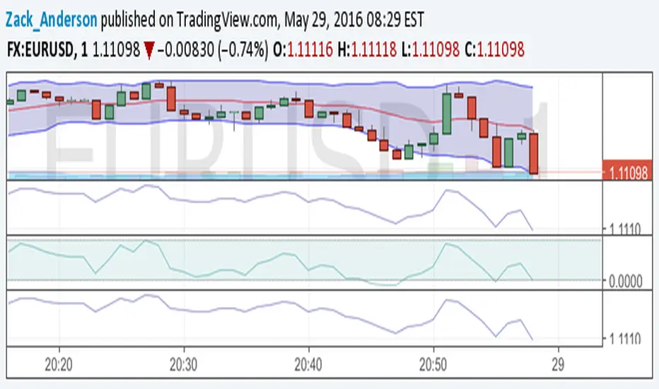
Bollinger Bands NEW
var tradingview_embed_options = {};
tradingview_embed_options.width = 640;
tradingview_embed_options.height = 400;
tradingview_embed_options.chart = 's48QJlfi';
new TradingView.chart(tradingview_embed_options);
Vdub Binary Options SniperVX v1 by vdubus on TradingView.com