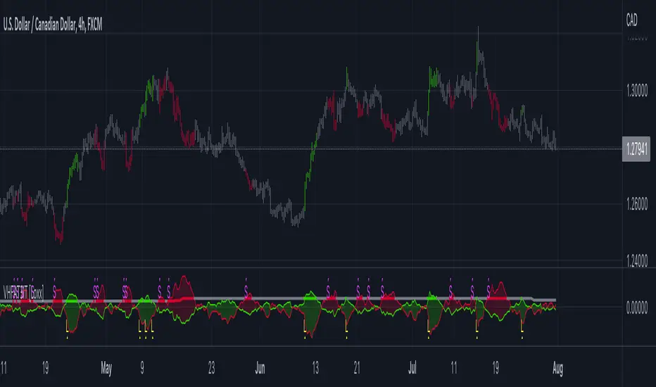
VHF-Adaptive T3 iTrend [Loxx]VHF-Adaptive T3 iTrend is an iTrend indicator with T3 smoothing and Vertical Horizontal Filter Adaptive period input. iTrend is used to determine where the trend starts and ends. You'll notice that the noise filter on this one is extreme. Adjust the period inputs accordingly to suit your take and your backtest requirements. This is also useful for scalping lower timeframes. Enjoy!
What is VHF Adaptive Period?
Vertical Horizontal Filter (VHF) was created by Adam White to identify trending and ranging markets. VHF measures the level of trend activity, similar to ADX DI. Vertical Horizontal Filter does not, itself, generate trading signals, but determines whether signals are taken from trend or momentum indicators. Using this trend information, one is then able to derive an average cycle length.
What is the T3 moving average?
Better Moving Averages Tim Tillson
November 1, 1998
Tim Tillson is a software project manager at Hewlett-Packard, with degrees in Mathematics and Computer Science. He has privately traded options and equities for 15 years.
Introduction
"Digital filtering includes the process of smoothing, predicting, differentiating, integrating, separation of signals, and removal of noise from a signal. Thus many people who do such things are actually using digital filters without realizing that they are; being unacquainted with the theory, they neither understand what they have done nor the possibilities of what they might have done."
This quote from R. W. Hamming applies to the vast majority of indicators in technical analysis . Moving averages, be they simple, weighted, or exponential, are lowpass filters; low frequency components in the signal pass through with little attenuation, while high frequencies are severely reduced.
"Oscillator" type indicators (such as MACD , Momentum, Relative Strength Index ) are another type of digital filter called a differentiator.
Tushar Chande has observed that many popular oscillators are highly correlated, which is sensible because they are trying to measure the rate of change of the underlying time series, i.e., are trying to be the first and second derivatives we all learned about in Calculus.
We use moving averages (lowpass filters) in technical analysis to remove the random noise from a time series, to discern the underlying trend or to determine prices at which we will take action. A perfect moving average would have two attributes:
It would be smooth, not sensitive to random noise in the underlying time series. Another way of saying this is that its derivative would not spuriously alternate between positive and negative values.
It would not lag behind the time series it is computed from. Lag, of course, produces late buy or sell signals that kill profits.
The only way one can compute a perfect moving average is to have knowledge of the future, and if we had that, we would buy one lottery ticket a week rather than trade!
Having said this, we can still improve on the conventional simple, weighted, or exponential moving averages. Here's how:
Two Interesting Moving Averages
We will examine two benchmark moving averages based on Linear Regression analysis.
In both cases, a Linear Regression line of length n is fitted to price data.
I call the first moving average ILRS, which stands for Integral of Linear Regression Slope. One simply integrates the slope of a linear regression line as it is successively fitted in a moving window of length n across the data, with the constant of integration being a simple moving average of the first n points. Put another way, the derivative of ILRS is the linear regression slope. Note that ILRS is not the same as a SMA ( simple moving average ) of length n, which is actually the midpoint of the linear regression line as it moves across the data.
We can measure the lag of moving averages with respect to a linear trend by computing how they behave when the input is a line with unit slope. Both SMA (n) and ILRS(n) have lag of n/2, but ILRS is much smoother than SMA .
Our second benchmark moving average is well known, called EPMA or End Point Moving Average. It is the endpoint of the linear regression line of length n as it is fitted across the data. EPMA hugs the data more closely than a simple or exponential moving average of the same length. The price we pay for this is that it is much noisier (less smooth) than ILRS, and it also has the annoying property that it overshoots the data when linear trends are present.
However, EPMA has a lag of 0 with respect to linear input! This makes sense because a linear regression line will fit linear input perfectly, and the endpoint of the LR line will be on the input line.
These two moving averages frame the tradeoffs that we are facing. On one extreme we have ILRS, which is very smooth and has considerable phase lag. EPMA has 0 phase lag, but is too noisy and overshoots. We would like to construct a better moving average which is as smooth as ILRS, but runs closer to where EPMA lies, without the overshoot.
A easy way to attempt this is to split the difference, i.e. use (ILRS(n)+EPMA(n))/2. This will give us a moving average (call it IE /2) which runs in between the two, has phase lag of n/4 but still inherits considerable noise from EPMA. IE /2 is inspirational, however. Can we build something that is comparable, but smoother? Figure 1 shows ILRS, EPMA, and IE /2.
Filter Techniques
Any thoughtful student of filter theory (or resolute experimenter) will have noticed that you can improve the smoothness of a filter by running it through itself multiple times, at the cost of increasing phase lag.
There is a complementary technique (called twicing by J.W. Tukey) which can be used to improve phase lag. If L stands for the operation of running data through a low pass filter, then twicing can be described by:
L' = L(time series) + L(time series - L(time series))
That is, we add a moving average of the difference between the input and the moving average to the moving average. This is algebraically equivalent to:
2L-L(L)
This is the Double Exponential Moving Average or DEMA , popularized by Patrick Mulloy in TASAC (January/February 1994).
In our taxonomy, DEMA has some phase lag (although it exponentially approaches 0) and is somewhat noisy, comparable to IE /2 indicator.
We will use these two techniques to construct our better moving average, after we explore the first one a little more closely.
Fixing Overshoot
An n-day EMA has smoothing constant alpha=2/(n+1) and a lag of (n-1)/2.
Thus EMA (3) has lag 1, and EMA (11) has lag 5. Figure 2 shows that, if I am willing to incur 5 days of lag, I get a smoother moving average if I run EMA (3) through itself 5 times than if I just take EMA (11) once.
This suggests that if EPMA and DEMA have 0 or low lag, why not run fast versions (eg DEMA (3)) through themselves many times to achieve a smooth result? The problem is that multiple runs though these filters increase their tendency to overshoot the data, giving an unusable result. This is because the amplitude response of DEMA and EPMA is greater than 1 at certain frequencies, giving a gain of much greater than 1 at these frequencies when run though themselves multiple times. Figure 3 shows DEMA (7) and EPMA(7) run through themselves 3 times. DEMA^3 has serious overshoot, and EPMA^3 is terrible.
The solution to the overshoot problem is to recall what we are doing with twicing:
DEMA (n) = EMA (n) + EMA (time series - EMA (n))
The second term is adding, in effect, a smooth version of the derivative to the EMA to achieve DEMA . The derivative term determines how hot the moving average's response to linear trends will be. We need to simply turn down the volume to achieve our basic building block:
EMA (n) + EMA (time series - EMA (n))*.7;
This is algebraically the same as:
EMA (n)*1.7-EMA( EMA (n))*.7;
I have chosen .7 as my volume factor, but the general formula (which I call "Generalized Dema") is:
GD (n,v) = EMA (n)*(1+v)-EMA( EMA (n))*v,
Where v ranges between 0 and 1. When v=0, GD is just an EMA , and when v=1, GD is DEMA . In between, GD is a cooler DEMA . By using a value for v less than 1 (I like .7), we cure the multiple DEMA overshoot problem, at the cost of accepting some additional phase delay. Now we can run GD through itself multiple times to define a new, smoother moving average T3 that does not overshoot the data:
T3(n) = GD ( GD ( GD (n)))
In filter theory parlance, T3 is a six-pole non-linear Kalman filter. Kalman filters are ones which use the error (in this case (time series - EMA (n)) to correct themselves. In Technical Analysis , these are called Adaptive Moving Averages; they track the time series more aggressively when it is making large moves.
Included
Bar coloring
Alerts
Signals
Loxx's Expanded Source Types
Pesquisar nos scripts por "TIM投资动向"
CFB-Adaptive CCI w/ T3 Smoothing [Loxx]CFB-Adaptive CCI w/ T3 Smoothing is a CCI indicator with adaptive period inputs and T3 smoothing. Jurik's Composite Fractal Behavior is used to created dynamic period input.
What is Composite Fractal Behavior ( CFB )?
All around you mechanisms adjust themselves to their environment. From simple thermostats that react to air temperature to computer chips in modern cars that respond to changes in engine temperature, r.p.m.'s, torque, and throttle position. It was only a matter of time before fast desktop computers applied the mathematics of self-adjustment to systems that trade the financial markets.
Unlike basic systems with fixed formulas, an adaptive system adjusts its own equations. For example, start with a basic channel breakout system that uses the highest closing price of the last N bars as a threshold for detecting breakouts on the up side. An adaptive and improved version of this system would adjust N according to market conditions, such as momentum, price volatility or acceleration.
Since many systems are based directly or indirectly on cycles, another useful measure of market condition is the periodic length of a price chart's dominant cycle, (DC), that cycle with the greatest influence on price action.
The utility of this new DC measure was noted by author Murray Ruggiero in the January '96 issue of Futures Magazine. In it. Mr. Ruggiero used it to adaptive adjust the value of N in a channel breakout system. He then simulated trading 15 years of D-Mark futures in order to compare its performance to a similar system that had a fixed optimal value of N. The adaptive version produced 20% more profit!
This DC index utilized the popular MESA algorithm (a formulation by John Ehlers adapted from Burg's maximum entropy algorithm, MEM). Unfortunately, the DC approach is problematic when the market has no real dominant cycle momentum, because the mathematics will produce a value whether or not one actually exists! Therefore, we developed a proprietary indicator that does not presuppose the presence of market cycles. It's called CFB (Composite Fractal Behavior) and it works well whether or not the market is cyclic.
CFB examines price action for a particular fractal pattern, categorizes them by size, and then outputs a composite fractal size index. This index is smooth, timely and accurate
Essentially, CFB reveals the length of the market's trending action time frame. Long trending activity produces a large CFB index and short choppy action produces a small index value. Investors have found many applications for CFB which involve scaling other existing technical indicators adaptively, on a bar-to-bar basis.
What is Jurik Volty used in the Juirk Filter?
One of the lesser known qualities of Juirk smoothing is that the Jurik smoothing process is adaptive. "Jurik Volty" (a sort of market volatility ) is what makes Jurik smoothing adaptive. The Jurik Volty calculation can be used as both a standalone indicator and to smooth other indicators that you wish to make adaptive.
What is the Jurik Moving Average?
Have you noticed how moving averages add some lag (delay) to your signals? ... especially when price gaps up or down in a big move, and you are waiting for your moving average to catch up? Wait no more! JMA eliminates this problem forever and gives you the best of both worlds: low lag and smooth lines.
Ideally, you would like a filtered signal to be both smooth and lag-free. Lag causes delays in your trades, and increasing lag in your indicators typically result in lower profits. In other words, late comers get what's left on the table after the feast has already begun.
What is the T3 moving average?
Better Moving Averages Tim Tillson
November 1, 1998
Tim Tillson is a software project manager at Hewlett-Packard, with degrees in Mathematics and Computer Science. He has privately traded options and equities for 15 years.
Introduction
"Digital filtering includes the process of smoothing, predicting, differentiating, integrating, separation of signals, and removal of noise from a signal. Thus many people who do such things are actually using digital filters without realizing that they are; being unacquainted with the theory, they neither understand what they have done nor the possibilities of what they might have done."
This quote from R. W. Hamming applies to the vast majority of indicators in technical analysis . Moving averages, be they simple, weighted, or exponential, are lowpass filters; low frequency components in the signal pass through with little attenuation, while high frequencies are severely reduced.
"Oscillator" type indicators (such as MACD , Momentum, Relative Strength Index ) are another type of digital filter called a differentiator.
Tushar Chande has observed that many popular oscillators are highly correlated, which is sensible because they are trying to measure the rate of change of the underlying time series, i.e., are trying to be the first and second derivatives we all learned about in Calculus.
We use moving averages (lowpass filters) in technical analysis to remove the random noise from a time series, to discern the underlying trend or to determine prices at which we will take action. A perfect moving average would have two attributes:
It would be smooth, not sensitive to random noise in the underlying time series. Another way of saying this is that its derivative would not spuriously alternate between positive and negative values.
It would not lag behind the time series it is computed from. Lag, of course, produces late buy or sell signals that kill profits.
The only way one can compute a perfect moving average is to have knowledge of the future, and if we had that, we would buy one lottery ticket a week rather than trade!
Having said this, we can still improve on the conventional simple, weighted, or exponential moving averages. Here's how:
Two Interesting Moving Averages
We will examine two benchmark moving averages based on Linear Regression analysis.
In both cases, a Linear Regression line of length n is fitted to price data.
I call the first moving average ILRS, which stands for Integral of Linear Regression Slope. One simply integrates the slope of a linear regression line as it is successively fitted in a moving window of length n across the data, with the constant of integration being a simple moving average of the first n points. Put another way, the derivative of ILRS is the linear regression slope. Note that ILRS is not the same as a SMA ( simple moving average ) of length n, which is actually the midpoint of the linear regression line as it moves across the data.
We can measure the lag of moving averages with respect to a linear trend by computing how they behave when the input is a line with unit slope. Both SMA (n) and ILRS(n) have lag of n/2, but ILRS is much smoother than SMA .
Our second benchmark moving average is well known, called EPMA or End Point Moving Average. It is the endpoint of the linear regression line of length n as it is fitted across the data. EPMA hugs the data more closely than a simple or exponential moving average of the same length. The price we pay for this is that it is much noisier (less smooth) than ILRS, and it also has the annoying property that it overshoots the data when linear trends are present.
However, EPMA has a lag of 0 with respect to linear input! This makes sense because a linear regression line will fit linear input perfectly, and the endpoint of the LR line will be on the input line.
These two moving averages frame the tradeoffs that we are facing. On one extreme we have ILRS, which is very smooth and has considerable phase lag. EPMA has 0 phase lag, but is too noisy and overshoots. We would like to construct a better moving average which is as smooth as ILRS, but runs closer to where EPMA lies, without the overshoot.
A easy way to attempt this is to split the difference, i.e. use (ILRS(n)+EPMA(n))/2. This will give us a moving average (call it IE /2) which runs in between the two, has phase lag of n/4 but still inherits considerable noise from EPMA. IE /2 is inspirational, however. Can we build something that is comparable, but smoother? Figure 1 shows ILRS, EPMA, and IE /2.
Filter Techniques
Any thoughtful student of filter theory (or resolute experimenter) will have noticed that you can improve the smoothness of a filter by running it through itself multiple times, at the cost of increasing phase lag.
There is a complementary technique (called twicing by J.W. Tukey) which can be used to improve phase lag. If L stands for the operation of running data through a low pass filter, then twicing can be described by:
L' = L(time series) + L(time series - L(time series))
That is, we add a moving average of the difference between the input and the moving average to the moving average. This is algebraically equivalent to:
2L-L(L)
This is the Double Exponential Moving Average or DEMA , popularized by Patrick Mulloy in TASAC (January/February 1994).
In our taxonomy, DEMA has some phase lag (although it exponentially approaches 0) and is somewhat noisy, comparable to IE /2 indicator.
We will use these two techniques to construct our better moving average, after we explore the first one a little more closely.
Fixing Overshoot
An n-day EMA has smoothing constant alpha=2/(n+1) and a lag of (n-1)/2.
Thus EMA (3) has lag 1, and EMA (11) has lag 5. Figure 2 shows that, if I am willing to incur 5 days of lag, I get a smoother moving average if I run EMA (3) through itself 5 times than if I just take EMA (11) once.
This suggests that if EPMA and DEMA have 0 or low lag, why not run fast versions (eg DEMA (3)) through themselves many times to achieve a smooth result? The problem is that multiple runs though these filters increase their tendency to overshoot the data, giving an unusable result. This is because the amplitude response of DEMA and EPMA is greater than 1 at certain frequencies, giving a gain of much greater than 1 at these frequencies when run though themselves multiple times. Figure 3 shows DEMA (7) and EPMA(7) run through themselves 3 times. DEMA^3 has serious overshoot, and EPMA^3 is terrible.
The solution to the overshoot problem is to recall what we are doing with twicing:
DEMA (n) = EMA (n) + EMA (time series - EMA (n))
The second term is adding, in effect, a smooth version of the derivative to the EMA to achieve DEMA . The derivative term determines how hot the moving average's response to linear trends will be. We need to simply turn down the volume to achieve our basic building block:
EMA (n) + EMA (time series - EMA (n))*.7;
This is algebraically the same as:
EMA (n)*1.7-EMA( EMA (n))*.7;
I have chosen .7 as my volume factor, but the general formula (which I call "Generalized Dema") is:
GD (n,v) = EMA (n)*(1+v)-EMA( EMA (n))*v,
Where v ranges between 0 and 1. When v=0, GD is just an EMA , and when v=1, GD is DEMA . In between, GD is a cooler DEMA . By using a value for v less than 1 (I like .7), we cure the multiple DEMA overshoot problem, at the cost of accepting some additional phase delay. Now we can run GD through itself multiple times to define a new, smoother moving average T3 that does not overshoot the data:
T3(n) = GD ( GD ( GD (n)))
In filter theory parlance, T3 is a six-pole non-linear Kalman filter. Kalman filters are ones which use the error (in this case (time series - EMA (n)) to correct themselves. In Technical Analysis , these are called Adaptive Moving Averages; they track the time series more aggressively when it is making large moves.
Included:
Bar coloring
Signals
Alerts

STD-Adaptive T3 Channel w/ Ehlers Swiss Army Knife Mod. [Loxx]STD-Adaptive T3 Channel w/ Ehlers Swiss Army Knife Mod. is an adaptive T3 indicator using standard deviation adaptivity and Ehlers Swiss Army Knife indicator to adjust the alpha value of the T3 calculation. This helps identify trends and reduce noise. In addition. I've included a Keltner Channel to show reversal/exhaustion zones.
What is the Swiss Army Knife Indicator?
John Ehlers explains the calculation here: www.mesasoftware.com
What is the T3 moving average?
Better Moving Averages Tim Tillson
November 1, 1998
Tim Tillson is a software project manager at Hewlett-Packard, with degrees in Mathematics and Computer Science. He has privately traded options and equities for 15 years.
Introduction
"Digital filtering includes the process of smoothing, predicting, differentiating, integrating, separation of signals, and removal of noise from a signal. Thus many people who do such things are actually using digital filters without realizing that they are; being unacquainted with the theory, they neither understand what they have done nor the possibilities of what they might have done."
This quote from R. W. Hamming applies to the vast majority of indicators in technical analysis . Moving averages, be they simple, weighted, or exponential, are lowpass filters; low frequency components in the signal pass through with little attenuation, while high frequencies are severely reduced.
"Oscillator" type indicators (such as MACD , Momentum, Relative Strength Index ) are another type of digital filter called a differentiator.
Tushar Chande has observed that many popular oscillators are highly correlated, which is sensible because they are trying to measure the rate of change of the underlying time series, i.e., are trying to be the first and second derivatives we all learned about in Calculus.
We use moving averages (lowpass filters) in technical analysis to remove the random noise from a time series, to discern the underlying trend or to determine prices at which we will take action. A perfect moving average would have two attributes:
It would be smooth, not sensitive to random noise in the underlying time series. Another way of saying this is that its derivative would not spuriously alternate between positive and negative values.
It would not lag behind the time series it is computed from. Lag, of course, produces late buy or sell signals that kill profits.
The only way one can compute a perfect moving average is to have knowledge of the future, and if we had that, we would buy one lottery ticket a week rather than trade!
Having said this, we can still improve on the conventional simple, weighted, or exponential moving averages. Here's how:
Two Interesting Moving Averages
We will examine two benchmark moving averages based on Linear Regression analysis.
In both cases, a Linear Regression line of length n is fitted to price data.
I call the first moving average ILRS, which stands for Integral of Linear Regression Slope. One simply integrates the slope of a linear regression line as it is successively fitted in a moving window of length n across the data, with the constant of integration being a simple moving average of the first n points. Put another way, the derivative of ILRS is the linear regression slope. Note that ILRS is not the same as a SMA ( simple moving average ) of length n, which is actually the midpoint of the linear regression line as it moves across the data.
We can measure the lag of moving averages with respect to a linear trend by computing how they behave when the input is a line with unit slope. Both SMA (n) and ILRS(n) have lag of n/2, but ILRS is much smoother than SMA .
Our second benchmark moving average is well known, called EPMA or End Point Moving Average. It is the endpoint of the linear regression line of length n as it is fitted across the data. EPMA hugs the data more closely than a simple or exponential moving average of the same length. The price we pay for this is that it is much noisier (less smooth) than ILRS, and it also has the annoying property that it overshoots the data when linear trends are present.
However, EPMA has a lag of 0 with respect to linear input! This makes sense because a linear regression line will fit linear input perfectly, and the endpoint of the LR line will be on the input line.
These two moving averages frame the tradeoffs that we are facing. On one extreme we have ILRS, which is very smooth and has considerable phase lag. EPMA has 0 phase lag, but is too noisy and overshoots. We would like to construct a better moving average which is as smooth as ILRS, but runs closer to where EPMA lies, without the overshoot.
A easy way to attempt this is to split the difference, i.e. use (ILRS(n)+EPMA(n))/2. This will give us a moving average (call it IE /2) which runs in between the two, has phase lag of n/4 but still inherits considerable noise from EPMA. IE /2 is inspirational, however. Can we build something that is comparable, but smoother? Figure 1 shows ILRS, EPMA, and IE /2.
Filter Techniques
Any thoughtful student of filter theory (or resolute experimenter) will have noticed that you can improve the smoothness of a filter by running it through itself multiple times, at the cost of increasing phase lag.
There is a complementary technique (called twicing by J.W. Tukey) which can be used to improve phase lag. If L stands for the operation of running data through a low pass filter, then twicing can be described by:
L' = L(time series) + L(time series - L(time series))
That is, we add a moving average of the difference between the input and the moving average to the moving average. This is algebraically equivalent to:
2L-L(L)
This is the Double Exponential Moving Average or DEMA , popularized by Patrick Mulloy in TASAC (January/February 1994).
In our taxonomy, DEMA has some phase lag (although it exponentially approaches 0) and is somewhat noisy, comparable to IE /2 indicator.
We will use these two techniques to construct our better moving average, after we explore the first one a little more closely.
Fixing Overshoot
An n-day EMA has smoothing constant alpha=2/(n+1) and a lag of (n-1)/2.
Thus EMA (3) has lag 1, and EMA (11) has lag 5. Figure 2 shows that, if I am willing to incur 5 days of lag, I get a smoother moving average if I run EMA (3) through itself 5 times than if I just take EMA (11) once.
This suggests that if EPMA and DEMA have 0 or low lag, why not run fast versions (eg DEMA (3)) through themselves many times to achieve a smooth result? The problem is that multiple runs though these filters increase their tendency to overshoot the data, giving an unusable result. This is because the amplitude response of DEMA and EPMA is greater than 1 at certain frequencies, giving a gain of much greater than 1 at these frequencies when run though themselves multiple times. Figure 3 shows DEMA (7) and EPMA(7) run through themselves 3 times. DEMA^3 has serious overshoot, and EPMA^3 is terrible.
The solution to the overshoot problem is to recall what we are doing with twicing:
DEMA (n) = EMA (n) + EMA (time series - EMA (n))
The second term is adding, in effect, a smooth version of the derivative to the EMA to achieve DEMA . The derivative term determines how hot the moving average's response to linear trends will be. We need to simply turn down the volume to achieve our basic building block:
EMA (n) + EMA (time series - EMA (n))*.7;
This is algebraically the same as:
EMA (n)*1.7-EMA( EMA (n))*.7;
I have chosen .7 as my volume factor, but the general formula (which I call "Generalized Dema") is:
GD (n,v) = EMA (n)*(1+v)-EMA( EMA (n))*v,
Where v ranges between 0 and 1. When v=0, GD is just an EMA , and when v=1, GD is DEMA . In between, GD is a cooler DEMA . By using a value for v less than 1 (I like .7), we cure the multiple DEMA overshoot problem, at the cost of accepting some additional phase delay. Now we can run GD through itself multiple times to define a new, smoother moving average T3 that does not overshoot the data:
T3(n) = GD ( GD ( GD (n)))
In filter theory parlance, T3 is a six-pole non-linear Kalman filter. Kalman filters are ones which use the error (in this case (time series - EMA (n)) to correct themselves. In Technical Analysis , these are called Adaptive Moving Averages; they track the time series more aggressively when it is making large moves.
Included:
Bar coloring
Signals
Alerts
Loxx's Expanded Source Types
T3 Velocity [Loxx]T3 Velocity is a simple velocity indicator using T3 moving average that uses gradient colors to better identify trends.
What is the T3 moving average?
Better Moving Averages Tim Tillson
November 1, 1998
Tim Tillson is a software project manager at Hewlett-Packard, with degrees in Mathematics and Computer Science. He has privately traded options and equities for 15 years.
Introduction
"Digital filtering includes the process of smoothing, predicting, differentiating, integrating, separation of signals, and removal of noise from a signal. Thus many people who do such things are actually using digital filters without realizing that they are; being unacquainted with the theory, they neither understand what they have done nor the possibilities of what they might have done."
This quote from R. W. Hamming applies to the vast majority of indicators in technical analysis . Moving averages, be they simple, weighted, or exponential, are lowpass filters; low frequency components in the signal pass through with little attenuation, while high frequencies are severely reduced.
"Oscillator" type indicators (such as MACD , Momentum, Relative Strength Index ) are another type of digital filter called a differentiator.
Tushar Chande has observed that many popular oscillators are highly correlated, which is sensible because they are trying to measure the rate of change of the underlying time series, i.e., are trying to be the first and second derivatives we all learned about in Calculus.
We use moving averages (lowpass filters) in technical analysis to remove the random noise from a time series, to discern the underlying trend or to determine prices at which we will take action. A perfect moving average would have two attributes:
It would be smooth, not sensitive to random noise in the underlying time series. Another way of saying this is that its derivative would not spuriously alternate between positive and negative values.
It would not lag behind the time series it is computed from. Lag, of course, produces late buy or sell signals that kill profits.
The only way one can compute a perfect moving average is to have knowledge of the future, and if we had that, we would buy one lottery ticket a week rather than trade!
Having said this, we can still improve on the conventional simple, weighted, or exponential moving averages. Here's how:
Two Interesting Moving Averages
We will examine two benchmark moving averages based on Linear Regression analysis.
In both cases, a Linear Regression line of length n is fitted to price data.
I call the first moving average ILRS, which stands for Integral of Linear Regression Slope. One simply integrates the slope of a linear regression line as it is successively fitted in a moving window of length n across the data, with the constant of integration being a simple moving average of the first n points. Put another way, the derivative of ILRS is the linear regression slope. Note that ILRS is not the same as a SMA ( simple moving average ) of length n, which is actually the midpoint of the linear regression line as it moves across the data.
We can measure the lag of moving averages with respect to a linear trend by computing how they behave when the input is a line with unit slope. Both SMA (n) and ILRS(n) have lag of n/2, but ILRS is much smoother than SMA .
Our second benchmark moving average is well known, called EPMA or End Point Moving Average. It is the endpoint of the linear regression line of length n as it is fitted across the data. EPMA hugs the data more closely than a simple or exponential moving average of the same length. The price we pay for this is that it is much noisier (less smooth) than ILRS, and it also has the annoying property that it overshoots the data when linear trends are present.
However, EPMA has a lag of 0 with respect to linear input! This makes sense because a linear regression line will fit linear input perfectly, and the endpoint of the LR line will be on the input line.
These two moving averages frame the tradeoffs that we are facing. On one extreme we have ILRS, which is very smooth and has considerable phase lag. EPMA has 0 phase lag, but is too noisy and overshoots. We would like to construct a better moving average which is as smooth as ILRS, but runs closer to where EPMA lies, without the overshoot.
A easy way to attempt this is to split the difference, i.e. use (ILRS(n)+EPMA(n))/2. This will give us a moving average (call it IE /2) which runs in between the two, has phase lag of n/4 but still inherits considerable noise from EPMA. IE /2 is inspirational, however. Can we build something that is comparable, but smoother? Figure 1 shows ILRS, EPMA, and IE /2.
Filter Techniques
Any thoughtful student of filter theory (or resolute experimenter) will have noticed that you can improve the smoothness of a filter by running it through itself multiple times, at the cost of increasing phase lag.
There is a complementary technique (called twicing by J.W. Tukey) which can be used to improve phase lag. If L stands for the operation of running data through a low pass filter, then twicing can be described by:
L' = L(time series) + L(time series - L(time series))
That is, we add a moving average of the difference between the input and the moving average to the moving average. This is algebraically equivalent to:
2L-L(L)
This is the Double Exponential Moving Average or DEMA , popularized by Patrick Mulloy in TASAC (January/February 1994).
In our taxonomy, DEMA has some phase lag (although it exponentially approaches 0) and is somewhat noisy, comparable to IE /2 indicator.
We will use these two techniques to construct our better moving average, after we explore the first one a little more closely.
Fixing Overshoot
An n-day EMA has smoothing constant alpha=2/(n+1) and a lag of (n-1)/2.
Thus EMA (3) has lag 1, and EMA (11) has lag 5. Figure 2 shows that, if I am willing to incur 5 days of lag, I get a smoother moving average if I run EMA (3) through itself 5 times than if I just take EMA (11) once.
This suggests that if EPMA and DEMA have 0 or low lag, why not run fast versions (eg DEMA (3)) through themselves many times to achieve a smooth result? The problem is that multiple runs though these filters increase their tendency to overshoot the data, giving an unusable result. This is because the amplitude response of DEMA and EPMA is greater than 1 at certain frequencies, giving a gain of much greater than 1 at these frequencies when run though themselves multiple times. Figure 3 shows DEMA (7) and EPMA(7) run through themselves 3 times. DEMA^3 has serious overshoot, and EPMA^3 is terrible.
The solution to the overshoot problem is to recall what we are doing with twicing:
DEMA (n) = EMA (n) + EMA (time series - EMA (n))
The second term is adding, in effect, a smooth version of the derivative to the EMA to achieve DEMA . The derivative term determines how hot the moving average's response to linear trends will be. We need to simply turn down the volume to achieve our basic building block:
EMA (n) + EMA (time series - EMA (n))*.7;
This is algebraically the same as:
EMA (n)*1.7-EMA( EMA (n))*.7;
I have chosen .7 as my volume factor, but the general formula (which I call "Generalized Dema") is:
GD (n,v) = EMA (n)*(1+v)-EMA( EMA (n))*v,
Where v ranges between 0 and 1. When v=0, GD is just an EMA , and when v=1, GD is DEMA . In between, GD is a cooler DEMA . By using a value for v less than 1 (I like .7), we cure the multiple DEMA overshoot problem, at the cost of accepting some additional phase delay. Now we can run GD through itself multiple times to define a new, smoother moving average T3 that does not overshoot the data:
T3(n) = GD ( GD ( GD (n)))
In filter theory parlance, T3 is a six-pole non-linear Kalman filter. Kalman filters are ones which use the error (in this case (time series - EMA (n)) to correct themselves. In Technical Analysis , these are called Adaptive Moving Averages; they track the time series more aggressively when it is making large moves.
Included:
Bar coloring
Signals
Alerts
Loxx's Expanded Source Types

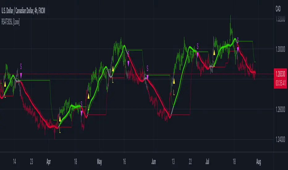
R-squared Adaptive T3 w/ DSL [Loxx]R-squared Adaptive T3 w/ DSL is the following T3 indicator but with Discontinued Signal Lines added to reduce noise and thereby increase signal accuracy. This adaptation makes this indicator lower TF scalp friendly.
What is R-squared Adaptive?
One tool available in forecasting the trendiness of the breakout is the coefficient of determination ( R-squared ), a statistical measurement.
The R-squared indicates linear strength between the security's price (the Y - axis) and time (the X - axis). The R-squared is the percentage of squared error that the linear regression can eliminate if it were used as the predictor instead of the mean value. If the R-squared were 0.99, then the linear regression would eliminate 99% of the error for prediction versus predicting closing prices using a simple moving average .
R-squared is used here to derive a T3 factor used to modify price before passing price through a six-pole non-linear Kalman filter.
What is the T3 moving average?
Better Moving Averages Tim Tillson
November 1, 1998
Tim Tillson is a software project manager at Hewlett-Packard, with degrees in Mathematics and Computer Science. He has privately traded options and equities for 15 years.
Introduction
"Digital filtering includes the process of smoothing, predicting, differentiating, integrating, separation of signals, and removal of noise from a signal. Thus many people who do such things are actually using digital filters without realizing that they are; being unacquainted with the theory, they neither understand what they have done nor the possibilities of what they might have done."
This quote from R. W. Hamming applies to the vast majority of indicators in technical analysis . Moving averages, be they simple, weighted, or exponential, are lowpass filters; low frequency components in the signal pass through with little attenuation, while high frequencies are severely reduced.
"Oscillator" type indicators (such as MACD , Momentum, Relative Strength Index ) are another type of digital filter called a differentiator.
Tushar Chande has observed that many popular oscillators are highly correlated, which is sensible because they are trying to measure the rate of change of the underlying time series, i.e., are trying to be the first and second derivatives we all learned about in Calculus.
We use moving averages (lowpass filters) in technical analysis to remove the random noise from a time series, to discern the underlying trend or to determine prices at which we will take action. A perfect moving average would have two attributes:
It would be smooth, not sensitive to random noise in the underlying time series. Another way of saying this is that its derivative would not spuriously alternate between positive and negative values.
It would not lag behind the time series it is computed from. Lag, of course, produces late buy or sell signals that kill profits.
The only way one can compute a perfect moving average is to have knowledge of the future, and if we had that, we would buy one lottery ticket a week rather than trade!
Having said this, we can still improve on the conventional simple, weighted, or exponential moving averages. Here's how:
Two Interesting Moving Averages
We will examine two benchmark moving averages based on Linear Regression analysis.
In both cases, a Linear Regression line of length n is fitted to price data.
I call the first moving average ILRS, which stands for Integral of Linear Regression Slope. One simply integrates the slope of a linear regression line as it is successively fitted in a moving window of length n across the data, with the constant of integration being a simple moving average of the first n points. Put another way, the derivative of ILRS is the linear regression slope. Note that ILRS is not the same as a SMA ( simple moving average ) of length n, which is actually the midpoint of the linear regression line as it moves across the data.
We can measure the lag of moving averages with respect to a linear trend by computing how they behave when the input is a line with unit slope. Both SMA (n) and ILRS(n) have lag of n/2, but ILRS is much smoother than SMA .
Our second benchmark moving average is well known, called EPMA or End Point Moving Average. It is the endpoint of the linear regression line of length n as it is fitted across the data. EPMA hugs the data more closely than a simple or exponential moving average of the same length. The price we pay for this is that it is much noisier (less smooth) than ILRS, and it also has the annoying property that it overshoots the data when linear trends are present.
However, EPMA has a lag of 0 with respect to linear input! This makes sense because a linear regression line will fit linear input perfectly, and the endpoint of the LR line will be on the input line.
These two moving averages frame the tradeoffs that we are facing. On one extreme we have ILRS, which is very smooth and has considerable phase lag. EPMA has 0 phase lag, but is too noisy and overshoots. We would like to construct a better moving average which is as smooth as ILRS, but runs closer to where EPMA lies, without the overshoot.
A easy way to attempt this is to split the difference, i.e. use (ILRS(n)+EPMA(n))/2. This will give us a moving average (call it IE /2) which runs in between the two, has phase lag of n/4 but still inherits considerable noise from EPMA. IE /2 is inspirational, however. Can we build something that is comparable, but smoother? Figure 1 shows ILRS, EPMA, and IE /2.
Filter Techniques
Any thoughtful student of filter theory (or resolute experimenter) will have noticed that you can improve the smoothness of a filter by running it through itself multiple times, at the cost of increasing phase lag.
There is a complementary technique (called twicing by J.W. Tukey) which can be used to improve phase lag. If L stands for the operation of running data through a low pass filter, then twicing can be described by:
L' = L(time series) + L(time series - L(time series))
That is, we add a moving average of the difference between the input and the moving average to the moving average. This is algebraically equivalent to:
2L-L(L)
This is the Double Exponential Moving Average or DEMA , popularized by Patrick Mulloy in TASAC (January/February 1994).
In our taxonomy, DEMA has some phase lag (although it exponentially approaches 0) and is somewhat noisy, comparable to IE /2 indicator.
We will use these two techniques to construct our better moving average, after we explore the first one a little more closely.
Fixing Overshoot
An n-day EMA has smoothing constant alpha=2/(n+1) and a lag of (n-1)/2.
Thus EMA (3) has lag 1, and EMA (11) has lag 5. Figure 2 shows that, if I am willing to incur 5 days of lag, I get a smoother moving average if I run EMA (3) through itself 5 times than if I just take EMA (11) once.
This suggests that if EPMA and DEMA have 0 or low lag, why not run fast versions (eg DEMA (3)) through themselves many times to achieve a smooth result? The problem is that multiple runs though these filters increase their tendency to overshoot the data, giving an unusable result. This is because the amplitude response of DEMA and EPMA is greater than 1 at certain frequencies, giving a gain of much greater than 1 at these frequencies when run though themselves multiple times. Figure 3 shows DEMA (7) and EPMA(7) run through themselves 3 times. DEMA^3 has serious overshoot, and EPMA^3 is terrible.
The solution to the overshoot problem is to recall what we are doing with twicing:
DEMA (n) = EMA (n) + EMA (time series - EMA (n))
The second term is adding, in effect, a smooth version of the derivative to the EMA to achieve DEMA . The derivative term determines how hot the moving average's response to linear trends will be. We need to simply turn down the volume to achieve our basic building block:
EMA (n) + EMA (time series - EMA (n))*.7;
This is algebraically the same as:
EMA (n)*1.7-EMA( EMA (n))*.7;
I have chosen .7 as my volume factor, but the general formula (which I call "Generalized Dema") is:
GD (n,v) = EMA (n)*(1+v)-EMA( EMA (n))*v,
Where v ranges between 0 and 1. When v=0, GD is just an EMA , and when v=1, GD is DEMA . In between, GD is a cooler DEMA . By using a value for v less than 1 (I like .7), we cure the multiple DEMA overshoot problem, at the cost of accepting some additional phase delay. Now we can run GD through itself multiple times to define a new, smoother moving average T3 that does not overshoot the data:
T3(n) = GD ( GD ( GD (n)))
In filter theory parlance, T3 is a six-pole non-linear Kalman filter. Kalman filters are ones which use the error (in this case (time series - EMA (n)) to correct themselves. In Technical Analysis , these are called Adaptive Moving Averages; they track the time series more aggressively when it is making large moves.
Included:
Bar coloring
Signals
Alerts
EMA and FEMA Signla/DSL smoothing
Loxx's Expanded Source Types
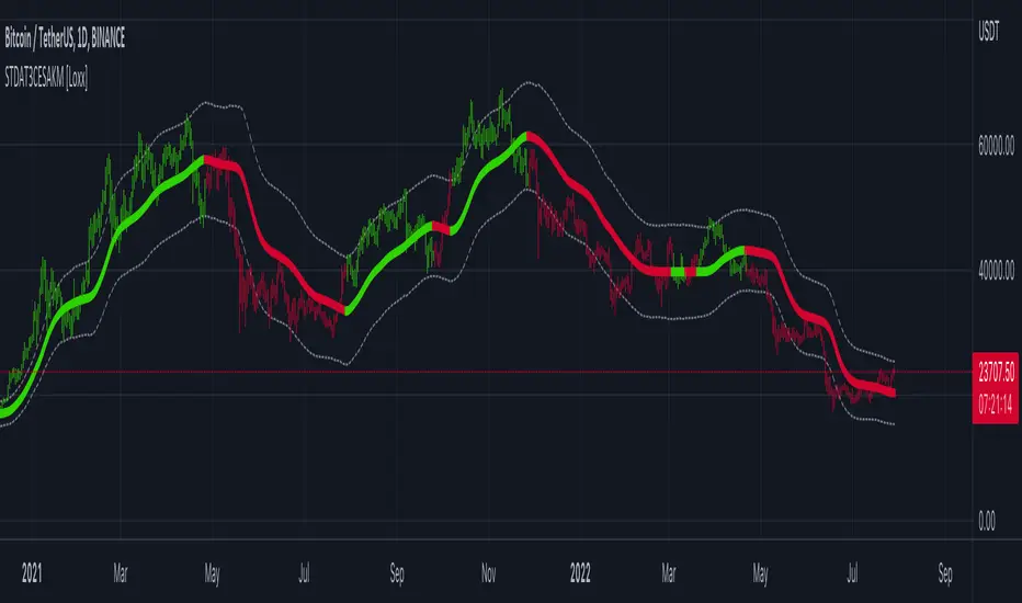
STD-Filterd, R-squared Adaptive T3 w/ Dynamic Zones [Loxx]STD-Filterd, R-squared Adaptive T3 w/ Dynamic Zones is a standard deviation filtered R-squared Adaptive T3 moving average with dynamic zones.
What is the T3 moving average?
Better Moving Averages Tim Tillson
November 1, 1998
Tim Tillson is a software project manager at Hewlett-Packard, with degrees in Mathematics and Computer Science. He has privately traded options and equities for 15 years.
Introduction
"Digital filtering includes the process of smoothing, predicting, differentiating, integrating, separation of signals, and removal of noise from a signal. Thus many people who do such things are actually using digital filters without realizing that they are; being unacquainted with the theory, they neither understand what they have done nor the possibilities of what they might have done."
This quote from R. W. Hamming applies to the vast majority of indicators in technical analysis . Moving averages, be they simple, weighted, or exponential, are lowpass filters; low frequency components in the signal pass through with little attenuation, while high frequencies are severely reduced.
"Oscillator" type indicators (such as MACD , Momentum, Relative Strength Index ) are another type of digital filter called a differentiator.
Tushar Chande has observed that many popular oscillators are highly correlated, which is sensible because they are trying to measure the rate of change of the underlying time series, i.e., are trying to be the first and second derivatives we all learned about in Calculus.
We use moving averages (lowpass filters) in technical analysis to remove the random noise from a time series, to discern the underlying trend or to determine prices at which we will take action. A perfect moving average would have two attributes:
It would be smooth, not sensitive to random noise in the underlying time series. Another way of saying this is that its derivative would not spuriously alternate between positive and negative values.
It would not lag behind the time series it is computed from. Lag, of course, produces late buy or sell signals that kill profits.
The only way one can compute a perfect moving average is to have knowledge of the future, and if we had that, we would buy one lottery ticket a week rather than trade!
Having said this, we can still improve on the conventional simple, weighted, or exponential moving averages. Here's how:
Two Interesting Moving Averages
We will examine two benchmark moving averages based on Linear Regression analysis.
In both cases, a Linear Regression line of length n is fitted to price data.
I call the first moving average ILRS, which stands for Integral of Linear Regression Slope. One simply integrates the slope of a linear regression line as it is successively fitted in a moving window of length n across the data, with the constant of integration being a simple moving average of the first n points. Put another way, the derivative of ILRS is the linear regression slope. Note that ILRS is not the same as a SMA ( simple moving average ) of length n, which is actually the midpoint of the linear regression line as it moves across the data.
We can measure the lag of moving averages with respect to a linear trend by computing how they behave when the input is a line with unit slope. Both SMA (n) and ILRS(n) have lag of n/2, but ILRS is much smoother than SMA .
Our second benchmark moving average is well known, called EPMA or End Point Moving Average. It is the endpoint of the linear regression line of length n as it is fitted across the data. EPMA hugs the data more closely than a simple or exponential moving average of the same length. The price we pay for this is that it is much noisier (less smooth) than ILRS, and it also has the annoying property that it overshoots the data when linear trends are present.
However, EPMA has a lag of 0 with respect to linear input! This makes sense because a linear regression line will fit linear input perfectly, and the endpoint of the LR line will be on the input line.
These two moving averages frame the tradeoffs that we are facing. On one extreme we have ILRS, which is very smooth and has considerable phase lag. EPMA has 0 phase lag, but is too noisy and overshoots. We would like to construct a better moving average which is as smooth as ILRS, but runs closer to where EPMA lies, without the overshoot.
A easy way to attempt this is to split the difference, i.e. use (ILRS(n)+EPMA(n))/2. This will give us a moving average (call it IE /2) which runs in between the two, has phase lag of n/4 but still inherits considerable noise from EPMA. IE /2 is inspirational, however. Can we build something that is comparable, but smoother? Figure 1 shows ILRS, EPMA, and IE /2.
Filter Techniques
Any thoughtful student of filter theory (or resolute experimenter) will have noticed that you can improve the smoothness of a filter by running it through itself multiple times, at the cost of increasing phase lag.
There is a complementary technique (called twicing by J.W. Tukey) which can be used to improve phase lag. If L stands for the operation of running data through a low pass filter, then twicing can be described by:
L' = L(time series) + L(time series - L(time series))
That is, we add a moving average of the difference between the input and the moving average to the moving average. This is algebraically equivalent to:
2L-L(L)
This is the Double Exponential Moving Average or DEMA , popularized by Patrick Mulloy in TASAC (January/February 1994).
In our taxonomy, DEMA has some phase lag (although it exponentially approaches 0) and is somewhat noisy, comparable to IE /2 indicator.
We will use these two techniques to construct our better moving average, after we explore the first one a little more closely.
Fixing Overshoot
An n-day EMA has smoothing constant alpha=2/(n+1) and a lag of (n-1)/2.
Thus EMA (3) has lag 1, and EMA (11) has lag 5. Figure 2 shows that, if I am willing to incur 5 days of lag, I get a smoother moving average if I run EMA (3) through itself 5 times than if I just take EMA (11) once.
This suggests that if EPMA and DEMA have 0 or low lag, why not run fast versions (eg DEMA (3)) through themselves many times to achieve a smooth result? The problem is that multiple runs though these filters increase their tendency to overshoot the data, giving an unusable result. This is because the amplitude response of DEMA and EPMA is greater than 1 at certain frequencies, giving a gain of much greater than 1 at these frequencies when run though themselves multiple times. Figure 3 shows DEMA (7) and EPMA(7) run through themselves 3 times. DEMA^3 has serious overshoot, and EPMA^3 is terrible.
The solution to the overshoot problem is to recall what we are doing with twicing:
DEMA (n) = EMA (n) + EMA (time series - EMA (n))
The second term is adding, in effect, a smooth version of the derivative to the EMA to achieve DEMA . The derivative term determines how hot the moving average's response to linear trends will be. We need to simply turn down the volume to achieve our basic building block:
EMA (n) + EMA (time series - EMA (n))*.7;
This is algebraically the same as:
EMA (n)*1.7-EMA( EMA (n))*.7;
I have chosen .7 as my volume factor, but the general formula (which I call "Generalized Dema") is:
GD (n,v) = EMA (n)*(1+v)-EMA( EMA (n))*v,
Where v ranges between 0 and 1. When v=0, GD is just an EMA , and when v=1, GD is DEMA . In between, GD is a cooler DEMA . By using a value for v less than 1 (I like .7), we cure the multiple DEMA overshoot problem, at the cost of accepting some additional phase delay. Now we can run GD through itself multiple times to define a new, smoother moving average T3 that does not overshoot the data:
T3(n) = GD ( GD ( GD (n)))
In filter theory parlance, T3 is a six-pole non-linear Kalman filter. Kalman filters are ones which use the error (in this case (time series - EMA (n)) to correct themselves. In Technical Analysis , these are called Adaptive Moving Averages; they track the time series more aggressively when it is making large moves.
What is R-squared Adaptive?
One tool available in forecasting the trendiness of the breakout is the coefficient of determination ( R-squared ), a statistical measurement.
The R-squared indicates linear strength between the security's price (the Y - axis) and time (the X - axis). The R-squared is the percentage of squared error that the linear regression can eliminate if it were used as the predictor instead of the mean value. If the R-squared were 0.99, then the linear regression would eliminate 99% of the error for prediction versus predicting closing prices using a simple moving average .
R-squared is used here to derive a T3 factor used to modify price before passing price through a six-pole non-linear Kalman filter.
What are Dynamic Zones?
As explained in "Stocks & Commodities V15:7 (306-310): Dynamic Zones by Leo Zamansky, Ph .D., and David Stendahl"
Most indicators use a fixed zone for buy and sell signals. Here’ s a concept based on zones that are responsive to past levels of the indicator.
One approach to active investing employs the use of oscillators to exploit tradable market trends. This investing style follows a very simple form of logic: Enter the market only when an oscillator has moved far above or below traditional trading lev- els. However, these oscillator- driven systems lack the ability to evolve with the market because they use fixed buy and sell zones. Traders typically use one set of buy and sell zones for a bull market and substantially different zones for a bear market. And therein lies the problem.
Once traders begin introducing their market opinions into trading equations, by changing the zones, they negate the system’s mechanical nature. The objective is to have a system automatically define its own buy and sell zones and thereby profitably trade in any market — bull or bear. Dynamic zones offer a solution to the problem of fixed buy and sell zones for any oscillator-driven system.
An indicator’s extreme levels can be quantified using statistical methods. These extreme levels are calculated for a certain period and serve as the buy and sell zones for a trading system. The repetition of this statistical process for every value of the indicator creates values that become the dynamic zones. The zones are calculated in such a way that the probability of the indicator value rising above, or falling below, the dynamic zones is equal to a given probability input set by the trader.
To better understand dynamic zones, let's first describe them mathematically and then explain their use. The dynamic zones definition:
Find V such that:
For dynamic zone buy: P{X <= V}=P1
For dynamic zone sell: P{X >= V}=P2
where P1 and P2 are the probabilities set by the trader, X is the value of the indicator for the selected period and V represents the value of the dynamic zone.
The probability input P1 and P2 can be adjusted by the trader to encompass as much or as little data as the trader would like. The smaller the probability, the fewer data values above and below the dynamic zones. This translates into a wider range between the buy and sell zones. If a 10% probability is used for P1 and P2, only those data values that make up the top 10% and bottom 10% for an indicator are used in the construction of the zones. Of the values, 80% will fall between the two extreme levels. Because dynamic zone levels are penetrated so infrequently, when this happens, traders know that the market has truly moved into overbought or oversold territory.
Calculating the Dynamic Zones
The algorithm for the dynamic zones is a series of steps. First, decide the value of the lookback period t. Next, decide the value of the probability Pbuy for buy zone and value of the probability Psell for the sell zone.
For i=1, to the last lookback period, build the distribution f(x) of the price during the lookback period i. Then find the value Vi1 such that the probability of the price less than or equal to Vi1 during the lookback period i is equal to Pbuy. Find the value Vi2 such that the probability of the price greater or equal to Vi2 during the lookback period i is equal to Psell. The sequence of Vi1 for all periods gives the buy zone. The sequence of Vi2 for all periods gives the sell zone.
In the algorithm description, we have: Build the distribution f(x) of the price during the lookback period i. The distribution here is empirical namely, how many times a given value of x appeared during the lookback period. The problem is to find such x that the probability of a price being greater or equal to x will be equal to a probability selected by the user. Probability is the area under the distribution curve. The task is to find such value of x that the area under the distribution curve to the right of x will be equal to the probability selected by the user. That x is the dynamic zone.
Included:
Bar coloring
Signals
Alerts
Loxx's Expanded Source Types

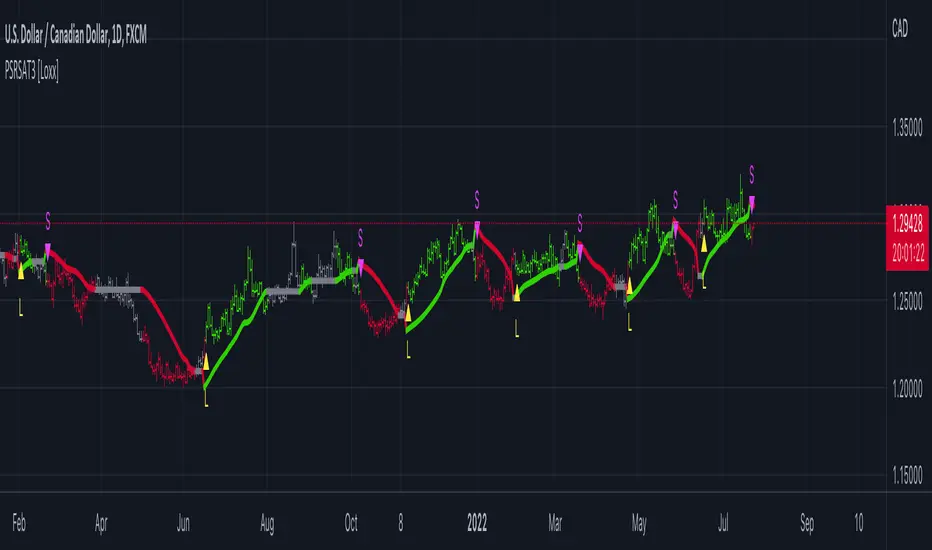
Pips-Stepped, R-squared Adaptive T3 [Loxx]Pips-Stepped, R-squared Adaptive T3 is a a T3 moving average with optional adaptivity, trend following, and pip-stepping. This indicator also uses optional flat coloring to determine chops zones. This indicator is R-squared adaptive. This is also an experimental indicator.
What is the T3 moving average?
Better Moving Averages Tim Tillson
November 1, 1998
Tim Tillson is a software project manager at Hewlett-Packard, with degrees in Mathematics and Computer Science. He has privately traded options and equities for 15 years.
Introduction
"Digital filtering includes the process of smoothing, predicting, differentiating, integrating, separation of signals, and removal of noise from a signal. Thus many people who do such things are actually using digital filters without realizing that they are; being unacquainted with the theory, they neither understand what they have done nor the possibilities of what they might have done."
This quote from R. W. Hamming applies to the vast majority of indicators in technical analysis . Moving averages, be they simple, weighted, or exponential, are lowpass filters; low frequency components in the signal pass through with little attenuation, while high frequencies are severely reduced.
"Oscillator" type indicators (such as MACD , Momentum, Relative Strength Index ) are another type of digital filter called a differentiator.
Tushar Chande has observed that many popular oscillators are highly correlated, which is sensible because they are trying to measure the rate of change of the underlying time series, i.e., are trying to be the first and second derivatives we all learned about in Calculus.
We use moving averages (lowpass filters) in technical analysis to remove the random noise from a time series, to discern the underlying trend or to determine prices at which we will take action. A perfect moving average would have two attributes:
It would be smooth, not sensitive to random noise in the underlying time series. Another way of saying this is that its derivative would not spuriously alternate between positive and negative values.
It would not lag behind the time series it is computed from. Lag, of course, produces late buy or sell signals that kill profits.
The only way one can compute a perfect moving average is to have knowledge of the future, and if we had that, we would buy one lottery ticket a week rather than trade!
Having said this, we can still improve on the conventional simple, weighted, or exponential moving averages. Here's how:
Two Interesting Moving Averages
We will examine two benchmark moving averages based on Linear Regression analysis.
In both cases, a Linear Regression line of length n is fitted to price data.
I call the first moving average ILRS, which stands for Integral of Linear Regression Slope. One simply integrates the slope of a linear regression line as it is successively fitted in a moving window of length n across the data, with the constant of integration being a simple moving average of the first n points. Put another way, the derivative of ILRS is the linear regression slope. Note that ILRS is not the same as a SMA ( simple moving average ) of length n, which is actually the midpoint of the linear regression line as it moves across the data.
We can measure the lag of moving averages with respect to a linear trend by computing how they behave when the input is a line with unit slope. Both SMA (n) and ILRS(n) have lag of n/2, but ILRS is much smoother than SMA .
Our second benchmark moving average is well known, called EPMA or End Point Moving Average. It is the endpoint of the linear regression line of length n as it is fitted across the data. EPMA hugs the data more closely than a simple or exponential moving average of the same length. The price we pay for this is that it is much noisier (less smooth) than ILRS, and it also has the annoying property that it overshoots the data when linear trends are present.
However, EPMA has a lag of 0 with respect to linear input! This makes sense because a linear regression line will fit linear input perfectly, and the endpoint of the LR line will be on the input line.
These two moving averages frame the tradeoffs that we are facing. On one extreme we have ILRS, which is very smooth and has considerable phase lag. EPMA has 0 phase lag, but is too noisy and overshoots. We would like to construct a better moving average which is as smooth as ILRS, but runs closer to where EPMA lies, without the overshoot.
A easy way to attempt this is to split the difference, i.e. use (ILRS(n)+EPMA(n))/2. This will give us a moving average (call it IE /2) which runs in between the two, has phase lag of n/4 but still inherits considerable noise from EPMA. IE /2 is inspirational, however. Can we build something that is comparable, but smoother? Figure 1 shows ILRS, EPMA, and IE /2.
Filter Techniques
Any thoughtful student of filter theory (or resolute experimenter) will have noticed that you can improve the smoothness of a filter by running it through itself multiple times, at the cost of increasing phase lag.
There is a complementary technique (called twicing by J.W. Tukey) which can be used to improve phase lag. If L stands for the operation of running data through a low pass filter, then twicing can be described by:
L' = L(time series) + L(time series - L(time series))
That is, we add a moving average of the difference between the input and the moving average to the moving average. This is algebraically equivalent to:
2L-L(L)
This is the Double Exponential Moving Average or DEMA , popularized by Patrick Mulloy in TASAC (January/February 1994).
In our taxonomy, DEMA has some phase lag (although it exponentially approaches 0) and is somewhat noisy, comparable to IE /2 indicator.
We will use these two techniques to construct our better moving average, after we explore the first one a little more closely.
Fixing Overshoot
An n-day EMA has smoothing constant alpha=2/(n+1) and a lag of (n-1)/2.
Thus EMA (3) has lag 1, and EMA (11) has lag 5. Figure 2 shows that, if I am willing to incur 5 days of lag, I get a smoother moving average if I run EMA (3) through itself 5 times than if I just take EMA (11) once.
This suggests that if EPMA and DEMA have 0 or low lag, why not run fast versions (eg DEMA (3)) through themselves many times to achieve a smooth result? The problem is that multiple runs though these filters increase their tendency to overshoot the data, giving an unusable result. This is because the amplitude response of DEMA and EPMA is greater than 1 at certain frequencies, giving a gain of much greater than 1 at these frequencies when run though themselves multiple times. Figure 3 shows DEMA (7) and EPMA(7) run through themselves 3 times. DEMA^3 has serious overshoot, and EPMA^3 is terrible.
The solution to the overshoot problem is to recall what we are doing with twicing:
DEMA (n) = EMA (n) + EMA (time series - EMA (n))
The second term is adding, in effect, a smooth version of the derivative to the EMA to achieve DEMA . The derivative term determines how hot the moving average's response to linear trends will be. We need to simply turn down the volume to achieve our basic building block:
EMA (n) + EMA (time series - EMA (n))*.7;
This is algebraically the same as:
EMA (n)*1.7-EMA( EMA (n))*.7;
I have chosen .7 as my volume factor, but the general formula (which I call "Generalized Dema") is:
GD (n,v) = EMA (n)*(1+v)-EMA( EMA (n))*v,
Where v ranges between 0 and 1. When v=0, GD is just an EMA , and when v=1, GD is DEMA . In between, GD is a cooler DEMA . By using a value for v less than 1 (I like .7), we cure the multiple DEMA overshoot problem, at the cost of accepting some additional phase delay. Now we can run GD through itself multiple times to define a new, smoother moving average T3 that does not overshoot the data:
T3(n) = GD ( GD ( GD (n)))
In filter theory parlance, T3 is a six-pole non-linear Kalman filter. Kalman filters are ones which use the error (in this case (time series - EMA (n)) to correct themselves. In Technical Analysis , these are called Adaptive Moving Averages; they track the time series more aggressively when it is making large moves.
What is R-squared Adaptive?
One tool available in forecasting the trendiness of the breakout is the coefficient of determination (R-squared), a statistical measurement.
The R-squared indicates linear strength between the security's price (the Y - axis) and time (the X - axis). The R-squared is the percentage of squared error that the linear regression can eliminate if it were used as the predictor instead of the mean value. If the R-squared were 0.99, then the linear regression would eliminate 99% of the error for prediction versus predicting closing prices using a simple moving average.
R-squared is used here to derive a T3 factor used to modify price before passing price through a six-pole non-linear Kalman filter.
Included:
Bar coloring
Signals
Alerts
Flat coloring
R-squared Adaptive T3 [Loxx]R-squared Adaptive T3 is an R-squared adaptive version of Tilson's T3 moving average. This adaptivity was originally proposed by mladen on various forex forums. This is considered experimental but shows how to use r-squared adapting methods to moving averages. In theory, the T3 is a six-pole non-linear Kalman filter.
What is the T3 moving average?
Better Moving Averages Tim Tillson
November 1, 1998
Tim Tillson is a software project manager at Hewlett-Packard, with degrees in Mathematics and Computer Science. He has privately traded options and equities for 15 years.
Introduction
"Digital filtering includes the process of smoothing, predicting, differentiating, integrating, separation of signals, and removal of noise from a signal. Thus many people who do such things are actually using digital filters without realizing that they are; being unacquainted with the theory, they neither understand what they have done nor the possibilities of what they might have done."
This quote from R. W. Hamming applies to the vast majority of indicators in technical analysis. Moving averages, be they simple, weighted, or exponential, are lowpass filters; low frequency components in the signal pass through with little attenuation, while high frequencies are severely reduced.
"Oscillator" type indicators (such as MACD, Momentum, Relative Strength Index) are another type of digital filter called a differentiator.
Tushar Chande has observed that many popular oscillators are highly correlated, which is sensible because they are trying to measure the rate of change of the underlying time series, i.e., are trying to be the first and second derivatives we all learned about in Calculus.
We use moving averages (lowpass filters) in technical analysis to remove the random noise from a time series, to discern the underlying trend or to determine prices at which we will take action. A perfect moving average would have two attributes:
It would be smooth, not sensitive to random noise in the underlying time series. Another way of saying this is that its derivative would not spuriously alternate between positive and negative values.
It would not lag behind the time series it is computed from. Lag, of course, produces late buy or sell signals that kill profits.
The only way one can compute a perfect moving average is to have knowledge of the future, and if we had that, we would buy one lottery ticket a week rather than trade!
Having said this, we can still improve on the conventional simple, weighted, or exponential moving averages. Here's how:
Two Interesting Moving Averages
We will examine two benchmark moving averages based on Linear Regression analysis.
In both cases, a Linear Regression line of length n is fitted to price data.
I call the first moving average ILRS, which stands for Integral of Linear Regression Slope. One simply integrates the slope of a linear regression line as it is successively fitted in a moving window of length n across the data, with the constant of integration being a simple moving average of the first n points. Put another way, the derivative of ILRS is the linear regression slope. Note that ILRS is not the same as a SMA (simple moving average) of length n, which is actually the midpoint of the linear regression line as it moves across the data.
We can measure the lag of moving averages with respect to a linear trend by computing how they behave when the input is a line with unit slope. Both SMA(n) and ILRS(n) have lag of n/2, but ILRS is much smoother than SMA.
Our second benchmark moving average is well known, called EPMA or End Point Moving Average. It is the endpoint of the linear regression line of length n as it is fitted across the data. EPMA hugs the data more closely than a simple or exponential moving average of the same length. The price we pay for this is that it is much noisier (less smooth) than ILRS, and it also has the annoying property that it overshoots the data when linear trends are present.
However, EPMA has a lag of 0 with respect to linear input! This makes sense because a linear regression line will fit linear input perfectly, and the endpoint of the LR line will be on the input line.
These two moving averages frame the tradeoffs that we are facing. On one extreme we have ILRS, which is very smooth and has considerable phase lag. EPMA has 0 phase lag, but is too noisy and overshoots. We would like to construct a better moving average which is as smooth as ILRS, but runs closer to where EPMA lies, without the overshoot.
A easy way to attempt this is to split the difference, i.e. use (ILRS(n)+EPMA(n))/2. This will give us a moving average (call it IE/2) which runs in between the two, has phase lag of n/4 but still inherits considerable noise from EPMA. IE/2 is inspirational, however. Can we build something that is comparable, but smoother? Figure 1 shows ILRS, EPMA, and IE/2.
Filter Techniques
Any thoughtful student of filter theory (or resolute experimenter) will have noticed that you can improve the smoothness of a filter by running it through itself multiple times, at the cost of increasing phase lag.
There is a complementary technique (called twicing by J.W. Tukey) which can be used to improve phase lag. If L stands for the operation of running data through a low pass filter, then twicing can be described by:
L' = L(time series) + L(time series - L(time series))
That is, we add a moving average of the difference between the input and the moving average to the moving average. This is algebraically equivalent to:
2L-L(L)
This is the Double Exponential Moving Average or DEMA, popularized by Patrick Mulloy in TASAC (January/February 1994).
In our taxonomy, DEMA has some phase lag (although it exponentially approaches 0) and is somewhat noisy, comparable to IE/2 indicator.
We will use these two techniques to construct our better moving average, after we explore the first one a little more closely.
Fixing Overshoot
An n-day EMA has smoothing constant alpha=2/(n+1) and a lag of (n-1)/2.
Thus EMA(3) has lag 1, and EMA(11) has lag 5. Figure 2 shows that, if I am willing to incur 5 days of lag, I get a smoother moving average if I run EMA(3) through itself 5 times than if I just take EMA(11) once.
This suggests that if EPMA and DEMA have 0 or low lag, why not run fast versions (eg DEMA(3)) through themselves many times to achieve a smooth result? The problem is that multiple runs though these filters increase their tendency to overshoot the data, giving an unusable result. This is because the amplitude response of DEMA and EPMA is greater than 1 at certain frequencies, giving a gain of much greater than 1 at these frequencies when run though themselves multiple times. Figure 3 shows DEMA(7) and EPMA(7) run through themselves 3 times. DEMA^3 has serious overshoot, and EPMA^3 is terrible.
The solution to the overshoot problem is to recall what we are doing with twicing:
DEMA(n) = EMA(n) + EMA(time series - EMA(n))
The second term is adding, in effect, a smooth version of the derivative to the EMA to achieve DEMA. The derivative term determines how hot the moving average's response to linear trends will be. We need to simply turn down the volume to achieve our basic building block:
EMA(n) + EMA(time series - EMA(n))*.7;
This is algebraically the same as:
EMA(n)*1.7-EMA(EMA(n))*.7;
I have chosen .7 as my volume factor, but the general formula (which I call "Generalized Dema") is:
GD(n,v) = EMA(n)*(1+v)-EMA(EMA(n))*v,
Where v ranges between 0 and 1. When v=0, GD is just an EMA, and when v=1, GD is DEMA. In between, GD is a cooler DEMA. By using a value for v less than 1 (I like .7), we cure the multiple DEMA overshoot problem, at the cost of accepting some additional phase delay. Now we can run GD through itself multiple times to define a new, smoother moving average T3 that does not overshoot the data:
T3(n) = GD(GD(GD(n)))
In filter theory parlance, T3 is a six-pole non-linear Kalman filter. Kalman filters are ones which use the error (in this case (time series - EMA(n)) to correct themselves. In Technical Analysis, these are called Adaptive Moving Averages; they track the time series more aggressively when it is making large moves.
Included:
Bar coloring
Signals
Alerts
Loxx's Expanded Source Types
Volume X-ray [LucF]█ OVERVIEW
This tool analyzes the relative size of volume reported on intraday vs EOD (end of day) data feeds on historical bars. If you use volume data to make trading decisions, it can help you improve your understanding of its nature and quality, which is especially important if you trade on intraday timeframes.
I often mention, when discussing volume analysis, how it's important for traders to understand the volume data they are using: where it originates, what it includes and does not include. By helping you spot sizeable differences between volume reported on intraday and EOD data feeds for any given instrument, "Volume X-ray" can point you to instruments where you might want to research the causes of the difference.
█ CONCEPTS
The information used to build a chart's historical bars originates from data providers (exchanges, brokers, etc.) who often maintain distinct historical feeds for intraday and EOD timeframes. How volume data is assembled for intraday and EOD feeds varies with instruments, brokers and exchanges. Variations between the two feeds — or their absence — can be due to how instruments are traded in a particular sector and/or the volume reporting policy for the feeds you are using. Instruments from crypto and forex markets, for example, will often display similar volume on both feeds. Stocks will often display variations because block trades or other types of trades may not be included in their intraday volume data. Futures will also typically display variations. It is even possible that volume from different feeds may not be of the same nature, as you can get trade volume (market volume) on one feed and tick volume (transaction counts) on another. You will sometimes be able to find the details of what different feeds contain from the technical information provided by exchanges/brokers on their feeds. This is an example for the NASDAQ feeds . Once you determine which feeds you are using, you can look for the reporting specs for that feed. This is all research you will need to do on your own; "Volume X-ray" will not help you with that part.
You may elect to forego the deep dive in feed information and simply rely on the figure the indicator will calculate for the instruments you trade. One simple — and unproven — way to interpret "Volume X-ray" values is to infer that instruments with larger percentages of intraday/EOD volume ratios are more "democratic" because at intraday timeframes, you are seeing a greater proportion of the actual traded volume for the instrument. This could conceivably lead one to conclude that such volume data is more reliable than on an instrument where intraday volume accounts for only 3% of EOD volume, let's say.
Note that as intraday vs EOD variations exist for historical bars on some instruments, there will typically also be differences between the realtime feeds used on intraday vs 1D or greater timeframes for those same assets. Realtime reporting rules will often be different from historical feed reporting rules, so variations between realtime feeds will often be different from the variations between historical feeds for the same instrument. A deep dive in reporting rules will quickly reveal what a jungle they are for some instruments, yet it is the only way to really understand the volume information our charts display.
█ HOW TO USE IT
The script is very simple and has no inputs. Just add it to 1D charts and it will calculate the proportion of volume reported on the intraday feed over the EOD volume. The plots show the daily values for both volumes: the teal area is the EOD volume, the orange line is the intraday volume. A value representing the average, cumulative intraday/EOD volume percentage for the chart is displayed in the upper-right corner. Its background color changes with the percentage, with brightness levels proportional to the percentage for both the bull color (% >= 50) or the bear color (% < 50). When abnormal conditions are detected, such as missing volume of one kind or the other, a yellow background is used.
Daily and cumulative values are displayed in indicator values and the Data Window.
The indicator loads in a pane, but you can also use it in overlay mode by moving it on the chart with "Move to" in the script's "More" menu, and disabling the plot display from the "Settings/Style" tab.
█ LIMITATIONS
• The script will not run on timeframes >1D because it cannot produce useful values on them.
• The calculation of the cumulative average will vary on different intraday timeframes because of the varying number of days covered by the dataset.
Variations can also occur because of irregularities in reported volume data. That is the reason I recommend using it on 1D charts.
• The script only calculates on historical bars because in real time there is no distinction between intraday and EOD feeds.
• You will see plenty of special cases if you use the indicator on a variety of instruments:
• Some instruments have no intraday volume, while on others it's the opposite.
• Missing information will sometimes appear here and there on datasets.
• Some instruments have higher intraday than EOD volume.
Please do not ask me the reasons for these anomalies; it's your responsibility to find them. I supply a tool that will spot the anomalies for you — nothing more.
█ FOR PINE CODERS
• This script uses a little-known feature of request.security() , which allows us to specify `"1440"` for the `timeframe` argument.
When you do, data from the 1min intrabars of the historical intraday feed is aggregated over one day, as opposed to the usual EOD feed used with `"D"`.
• I use gaps on my request.security() calls. This is useful because at intraday timeframes I can cumulate non- na values only.
• I use fixnan() on some values. For those who don't know about it yet, it eliminates na values from a series, just like not using gaps will do in a request.security() call.
• I like how the new switch structure makes for more readable code than equivalent if structures.
• I wrote my script using the revised recommendations in the Style Guide from the Pine v5 User Manual.
• I use the new runtime.error() to throw an error when the script user tries to use a timeframe >1D.
Why? Because then, my request.security() calls would be returning values from the last 1D intrabar of the dilation of the, let's say, 1W chart bar.
This of course would be of no use whatsoever — and misleading. I encourage all Pine coders fetching HTF data to protect their script users in the same way.
As tool builders, it is our responsibility to shield unsuspecting users of our scripts from contexts where our calcs produce invalid results.
• While we're on the subject of accessing intrabar timeframes, I will add this to the intention of coders falling victim to what appears to be
a new misconception where the mere fact of using intrabar timeframes with request.security() is believed to provide some sort of edge.
This is a fallacy unless you are sending down functions specifically designed to mine values from request.security() 's intrabar context.
These coders do not seem to realize that:
• They are only retrieving information from the last intrabar of the chart bar.
• The already flawed behavior of their scripts on historical bars will not improve on realtime bars. It will actually worsen because in real time,
intrabars are not yet ordered sequentially as they are on historical bars.
• Alerts or strategy orders using intrabar information acquired through request.security() will be using flawed logic and data most of the time.
The situation reminds me of the mania where using Heikin-Ashi charts to backtest was all the rage because it produced magnificent — and flawed — results.
Trading is difficult enough when doing the right things; I hate to see traders infected by lethal beliefs.
Strive to sharpen your "herd immunity", as Lionel Shriver calls it. She also writes: "Be leery of orthodoxy. Hold back from shared cultural enthusiasms."
Be your own trader.
█ THANKS
This indicator would not exist without the invaluable insights from Tim, a member of the Pine team. Thanks Tim!
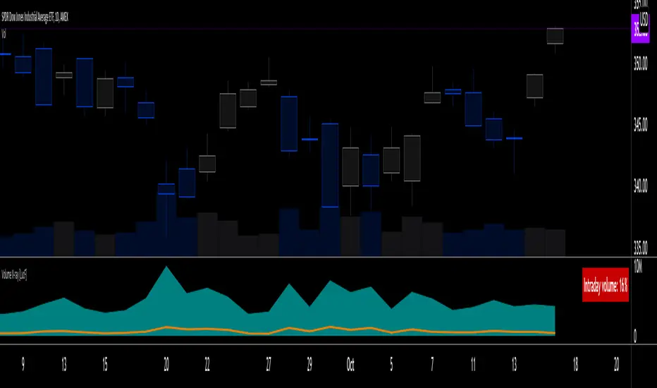
Combo Backtest 123 Reversal & T3 Averages This is combo strategies for get a cumulative signal.
First strategy
This System was created from the Book "How I Tripled My Money In The
Futures Market" by Ulf Jensen, Page 183. This is reverse type of strategies.
The strategy buys at market, if close price is higher than the previous close
during 2 days and the meaning of 9-days Stochastic Slow Oscillator is lower than 50.
The strategy sells at market, if close price is lower than the previous close price
during 2 days and the meaning of 9-days Stochastic Fast Oscillator is higher than 50.
Second strategy
This indicator plots the moving average described in the January, 1998 issue
of S&C, p.57, "Smoothing Techniques for More Accurate Signals", by Tim Tillson.
This indicator plots T3 moving average presented in Figure 4 in the article.
T3 indicator is a moving average which is calculated according to formula:
T3(n) = GD(GD(GD(n))),
where GD - generalized DEMA (Double EMA) and calculating according to this:
GD(n,v) = EMA(n) * (1+v)-EMA(EMA(n)) * v,
where "v" is volume factor, which determines how hot the moving average’s response
to linear trends will be. The author advises to use v=0.7.
When v = 0, GD = EMA, and when v = 1, GD = DEMA. In between, GD is a less aggressive
version of DEMA. By using a value for v less than1, trader cure the multiple DEMA
overshoot problem but at the cost of accepting some additional phase delay.
In filter theory terminology, T3 is a six-pole nonlinear Kalman filter. Kalman
filters are ones that use the error — in this case, (time series - EMA(n)) —
to correct themselves. In the realm of technical analysis, these are called adaptive
moving averages; they track the time series more aggres-sively when it is making large
moves. Tim Tillson is a software project manager at Hewlett-Packard, with degrees in
mathematics and computer science. He has privately traded options and equities for 15 years.
WARNING:
- For purpose educate only
- This script to change bars colors.
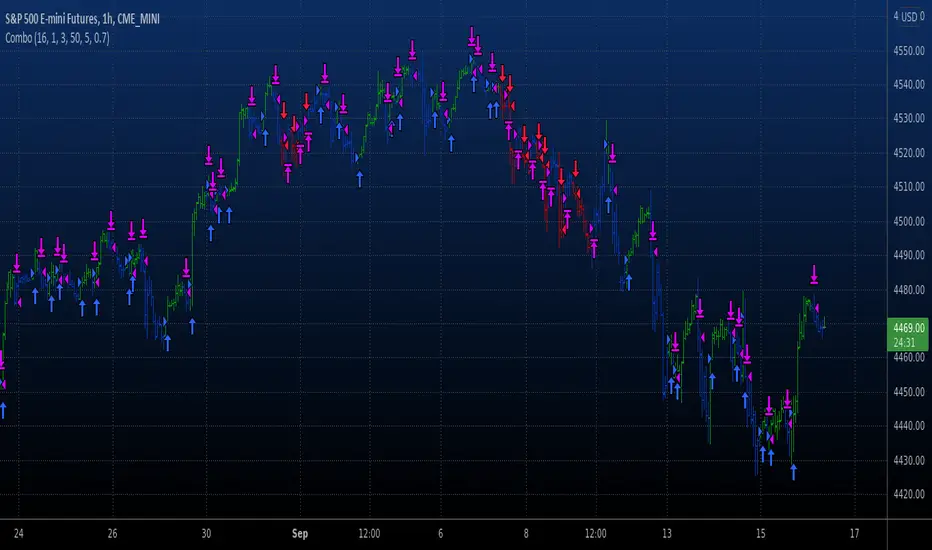
Tillson T3 Moving Average MTFMULTIPLE TIME FRAME version of Tillson T3 Moving Average Indicator
Developed by Tim Tillson, the T3 Moving Average is considered superior -1.60% to traditional moving averages as it is smoother, more responsive and thus performs better in ranging market conditions as well. However, it bears the disadvantage of overshooting the price as it attempts to realign itself to current market conditions.
It incorporates a smoothing technique which allows it to plot curves more gradual than ordinary moving averages and with a smaller lag. Its smoothness is derived from the fact that it is a weighted sum of a single EMA , double EMA , triple EMA and so on. When a trend is formed, the price action will stay above or below the trend during most of its progression and will hardly be touched by any swings. Thus, a confirmed penetration of the T3 MA and the lack of a following reversal often indicates the end of a trend.
The T3 Moving Average generally produces entry signals similar to other moving averages and thus is traded largely in the same manner. Here are several assumptions:
If the price action is above the T3 Moving Average and the indicator is headed upward, then we have a bullish trend and should only enter long trades (advisable for novice/intermediate traders). If the price is below the T3 Moving Average and it is edging lower, then we have a bearish trend and should limit entries to short. Below you can see it visualized in a trading platform.
Although the T3 MA is considered as one of the best swing following indicators that can be used on all time frames and in any market, it is still not advisable for novice/intermediate traders to increase their risk level and enter the market during trading ranges (especially tight ones). Thus, for the purposes of this article we will limit our entry signals only to such in trending conditions.
Once the market is displaying trending behavior, we can place with-trend entry orders as soon as the price pulls back to the moving average (undershooting or overshooting it will also work). As we know, moving averages are strong resistance/support levels, thus the price is more likely to rebound from them and resume its with-trend direction instead of penetrating it and reversing the trend.
And so, in a bull trend, if the market pulls back to the moving average, we can fairly safely assume that it will bounce off the T3 MA and resume upward momentum, thus we can go long. The same logic is in force during a bearish trend .
And last but not least, the T3 Moving Average can be used to generate entry signals upon crossing with another T3 MA with a longer trackback period (just like any other moving average crossover). When the fast T3 crosses the slower one from below and edges higher, this is called a Golden Cross and produces a bullish entry signal. When the faster T3 crosses the slower one from above and declines further, the scenario is called a Death Cross and signifies bearish conditions.
I Personally added a second T3 line with a volume factor of 0.618 (Fibonacci Ratio) and length of 3 (fibonacci number) which can be added by selecting the box in the input section. traders can combine the two lines to have Buy/Sell signals from the crosses.
Developed by Tim Tillson

Tillson T3 Moving Average by KIVANÇ fr3762Developed by Tim Tillson, the T3 Moving Average is considered superior to traditional moving averages as it is smoother, more responsive and thus performs better in ranging market conditions as well. However, it bears the disadvantage of overshooting the price as it attempts to realign itself to current market conditions.
It incorporates a smoothing technique which allows it to plot curves more gradual than ordinary moving averages and with a smaller lag. Its smoothness is derived from the fact that it is a weighted sum of a single EMA , double EMA , triple EMA and so on. When a trend is formed, the price action will stay above or below the trend during most of its progression and will hardly be touched by any swings. Thus, a confirmed penetration of the T3 MA and the lack of a following reversal often indicates the end of a trend.
The T3 Moving Average generally produces entry signals similar to other moving averages and thus is traded largely in the same manner. Here are several assumptions:
If the price action is above the T3 Moving Average and the indicator is headed upward, then we have a bullish trend and should only enter long trades (advisable for novice/intermediate traders). If the price is below the T3 Moving Average and it is edging lower, then we have a bearish trend and should limit entries to short. Below you can see it visualized in a trading platform.
Although the T3 MA is considered as one of the best swing following indicators that can be used on all time frames and in any market, it is still not advisable for novice/intermediate traders to increase their risk level and enter the market during trading ranges (especially tight ones). Thus, for the purposes of this article we will limit our entry signals only to such in trending conditions.
Once the market is displaying trending behavior, we can place with-trend entry orders as soon as the price pulls back to the moving average (undershooting or overshooting it will also work). As we know, moving averages are strong resistance/support levels, thus the price is more likely to rebound from them and resume its with-trend direction instead of penetrating it and reversing the trend.
And so, in a bull trend, if the market pulls back to the moving average, we can fairly safely assume that it will bounce off the T3 MA and resume upward momentum, thus we can go long. The same logic is in force during a bearish trend .
And last but not least, the T3 Moving Average can be used to generate entry signals upon crossing with another T3 MA with a longer trackback period (just like any other moving average crossover). When the fast T3 crosses the slower one from below and edges higher, this is called a Golden Cross and produces a bullish entry signal. When the faster T3 crosses the slower one from above and declines further, the scenario is called a Death Cross and signifies bearish conditions.
I Personally added a second T3 line with a volume factor of 0.618 (Fibonacci Ratio) and length of 3 (fibonacci number) which can be added by selecting the box in the input section. traders can combine the two lines to have Buy/Sell signals from the crosses.
Developed by Tim Tillson
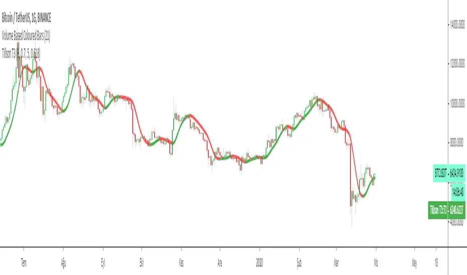
T3 Averages Backtest This indicator plots the moving average described in the January, 1998 issue
of S&C, p.57, "Smoothing Techniques for More Accurate Signals", by Tim Tillson.
This indicator plots T3 moving average presented in Figure 4 in the article.
T3 indicator is a moving average which is calculated according to formula:
T3(n) = GD(GD(GD(n))),
where GD - generalized DEMA (Double EMA) and calculating according to this:
GD(n,v) = EMA(n) * (1+v)-EMA(EMA(n)) * v,
where "v" is volume factor, which determines how hot the moving average’s response
to linear trends will be. The author advises to use v=0.7.
When v = 0, GD = EMA, and when v = 1, GD = DEMA. In between, GD is a less aggressive
version of DEMA. By using a value for v less than1, trader cure the multiple DEMA
overshoot problem but at the cost of accepting some additional phase delay.
In filter theory terminology, T3 is a six-pole nonlinear Kalman filter. Kalman
filters are ones that use the error — in this case, (time series - EMA(n)) —
to correct themselves. In the realm of technical analysis, these are called adaptive
moving averages; they track the time series more aggres-sively when it is making large
moves. Tim Tillson is a software project manager at Hewlett-Packard, with degrees in
mathematics and computer science. He has privately traded options and equities for 15 years.
You can change long to short in the Input Settings
WARNING:
- For purpose educate only
- This script to change bars colors.
T3 Averages Strategy This indicator plots the moving average described in the January, 1998 issue
of S&C, p.57, "Smoothing Techniques for More Accurate Signals", by Tim Tillson.
This indicator plots T3 moving average presented in Figure 4 in the article.
T3 indicator is a moving average which is calculated according to formula:
T3(n) = GD(GD(GD(n))),
where GD - generalized DEMA (Double EMA) and calculating according to this:
GD(n,v) = EMA(n) * (1+v)-EMA(EMA(n)) * v,
where "v" is volume factor, which determines how hot the moving average’s response
to linear trends will be. The author advises to use v=0.7.
When v = 0, GD = EMA, and when v = 1, GD = DEMA. In between, GD is a less aggressive
version of DEMA. By using a value for v less than1, trader cure the multiple DEMA
overshoot problem but at the cost of accepting some additional phase delay.
In filter theory terminology, T3 is a six-pole nonlinear Kalman filter. Kalman
filters are ones that use the error — in this case, (time series - EMA(n)) —
to correct themselves. In the realm of technical analysis, these are called adaptive
moving averages; they track the time series more aggres-sively when it is making large
moves. Tim Tillson is a software project manager at Hewlett-Packard, with degrees in
mathematics and computer science. He has privately traded options and equities for 15 years.
WARNING:
- This script to change bars colors.
TimWest Long Short FiltersTimWest Long Short Filters
Indicator Has 3 Separate Filters that Create Green(Bullish) or Red(Bearish) BackGround Highlights
If Price is Above or Below a certain LookBack Period - Tim Defaults to 63 on Daily Chart to Quickly View if Price is Above or Below it’s Price 1 Quarter Ago.
A Simple Moving Average Filter - Tim Defaults to 50 SMA and 200 SMA also known as the “Golden Cross”.
A Exponential Moving Average Filter - For Those Who Want To View Shorter Term Market Swings. Defaults to 50 EMA and 100 EMA used By Chuck Hughes, 7 Time World Trading Champion. Chuck Claims the 50/100 EMA's Show the Earliest Change in Market Direction the Equal - Sustainable Moves
Inputs Tab has Checkboxes to Turn On/Off any of the 3 Filters Above.
Reference Chart Post www.tradingview.com

T3 Average This indicator plots the moving average described in the January, 1998 issue
of S&C, p.57, "Smoothing Techniques for More Accurate Signals", by Tim Tillson.
This indicator plots T3 moving average presented in Figure 4 in the article.
T3 indicator is a moving average which is calculated according to formula:
T3(n) = GD(GD(GD(n))),
where GD - generalized DEMA (Double EMA) and calculating according to this:
GD(n,v) = EMA(n) * (1+v)-EMA(EMA(n)) * v,
where "v" is volume factor, which determines how hot the moving average’s response
to linear trends will be. The author advises to use v=0.7.
When v = 0, GD = EMA, and when v = 1, GD = DEMA. In between, GD is a less aggressive
version of DEMA. By using a value for v less than1, trader cure the multiple DEMA
overshoot problem but at the cost of accepting some additional phase delay.
In filter theory terminology, T3 is a six-pole nonlinear Kalman filter. Kalman
filters are ones that use the error — in this case, (time series - EMA(n)) —
to correct themselves. In the realm of technical analysis, these are called adaptive
moving averages; they track the time series more aggres-sively when it is making large
moves. Tim Tillson is a software project manager at Hewlett-Packard, with degrees in
mathematics and computer science. He has privately traded options and equities for 15 years.
RSI of RSI Deviation (RoRD)RSI of RSI Deviation (RoRD) - Advanced Momentum Acceleration Analysis
What is RSI of RSI Deviation (RoRD)?
RSI of RSI Deviation (RoRD) is a insightful momentum indicator that transcends traditional oscillator analysis by measuring the acceleration of momentum through sophisticated mathematical layering. By calculating RSI on RSI itself (RSI²) and applying advanced statistical deviation analysis with T3 smoothing, RoRD reveals hidden market dynamics that single-layer indicators miss entirely.
This isn't just another RSI variant—it's a complete reimagining of how we measure and visualize momentum dynamics. Where traditional RSI shows momentum, RoRD shows momentum's rate of change . Where others show static overbought/oversold levels, RoRD reveals statistically significant deviations unique to each market's character.
Theoretical Foundation - The Mathematics of Momentum Acceleration
1. RSI² (RSI of RSI) - The Core Innovation
Traditional RSI measures price momentum. RoRD goes deeper:
Primary RSI (RSI₁) : Standard RSI calculation on price
Secondary RSI (RSI²) : RSI calculated on RSI₁ values
This creates a "momentum of momentum" indicator that leads price action
Mathematical Expression:
RSI₁ = 100 - (100 / (1 + RS₁))
RSI² = 100 - (100 / (1 + RS₂))
Where RS₂ = Average Gain of RSI₁ / Average Loss of RSI₁
2. T3 Smoothing - Lag-Free Response
The T3 Moving Average, developed by Tim Tillson, provides:
Superior smoothing with minimal lag
Adaptive response through volume factor (vFactor)
Noise reduction while preserving signal integrity
T3 Formula:
T3 = c1×e6 + c2×e5 + c3×e4 + c4×e3
Where e1...e6 are cascaded EMAs and c1...c4 are volume-factor-based coefficients
3. Statistical Z-Score Deviation
RoRD employs dual-layer Z-score normalization :
Initial Z-Score : (RSI² - SMA) / StDev
Final Z-Score : Z-score of the Z-score for refined extremity detection
This identifies statistically rare events relative to recent market behavior
4. Multi-Timeframe Confluence
Compares current timeframe Z-score with higher timeframe (HTF)
Provides directional confirmation across time horizons
Filters false signals through timeframe alignment
Why RoRD is Different & More Sophisticated
Beyond Traditional Indicators:
Acceleration vs. Velocity : While RSI measures momentum (velocity), RoRD measures momentum's rate of change (acceleration)
Adaptive Thresholds : Z-score analysis adapts to market conditions rather than using fixed 70/30 levels
Statistical Significance : Signals are based on mathematical rarity, not arbitrary levels
Leading Indicator : RSI² often turns before price, providing earlier signals
Reduced Whipsaws : T3 smoothing eliminates noise while maintaining responsiveness
Unique Signal Generation:
Quantum Orbs : Multi-layered visual signals for statistically extreme events
Divergence Detection : Automated identification of price/momentum divergences
Regime Backgrounds : Visual market state classification (Bullish/Bearish/Neutral)
Particle Effects : Dynamic visualization of momentum energy
Visual Design & Interpretation Guide
Color Coding System:
Yellow (#e1ff00) : Neutral/balanced momentum state
Red (#ff0000) : Overbought/extreme bullish acceleration
Green (#2fff00) : Oversold/extreme bearish acceleration
Orange : Z-score visualization
Blue : HTF Z-score comparison
Main Visual Elements:
RSI² Line with Glow Effect
Multi-layer glow creates depth and emphasis
Color dynamically shifts based on momentum state
Line thickness indicates signal strength
Quantum Signal Orbs
Green Orbs Below : Statistically rare oversold conditions
Red Orbs Above : Statistically rare overbought conditions
Multiple layers indicate signal strength
Only appear at Z-score extremes for high-conviction signals
Divergence Markers
Green Circles : Bullish divergence detected
Red Circles : Bearish divergence detected
Plotted at pivot points for precision
Background Regimes
Green Background : Bullish momentum regime
Grey Background : Bearish momentum regime
Blue Background : Neutral/transitioning regime
Particle Effects
Density indicates momentum energy
Color matches current RSI² state
Provides dynamic market "feel"
Dashboard Metrics - Deep Dive
RSI² ANALYSIS Section:
RSI² Value (0-100)
Current smoothed RSI of RSI reading
>70 : Strong bullish acceleration
<30 : Strong bearish acceleration
~50 : Neutral momentum state
RSI¹ Value
Traditional RSI for reference
Compare with RSI² for acceleration/deceleration insights
Z-Score Status
🔥 EXTREME HIGH : Z > threshold, statistically rare bullish
❄️ EXTREME LOW : Z < threshold, statistically rare bearish
📈 HIGH/📉 LOW : Elevated but not extreme
➡️ NEUTRAL : Normal statistical range
MOMENTUM Section:
Velocity Indicator
▲▲▲ : Strong positive acceleration
▼▼▼ : Strong negative acceleration
Shows rate of change in RSI²
Strength Bar
██████░░░░ : Visual power gauge
Filled bars indicate momentum strength
Based on deviation from center line
SIGNALS Section:
Divergence Status
🟢 BULLISH DIV : Price making lows, RSI² making highs
🔴 BEARISH DIV : Price making highs, RSI² making lows
⚪ NO DIVERGENCE : No divergence detected
HTF Comparison
🔥 HTF EXTREME : Higher timeframe confirms extremity
📊 HTF NORMAL : Higher timeframe is neutral
Critical for multi-timeframe confirmation
Trading Application & Strategy
Signal Hierarchy (Highest to Lowest Priority):
Quantum Orb + HTF Alignment + Divergence
Highest conviction reversal signal
Z-score extreme + timeframe confluence + divergence
Quantum Orb + HTF Alignment
Strong reversal signal
Wait for price confirmation
Divergence + Regime Change
Medium-term reversal signal
Monitor for orb confirmation
Threshold Crosses
Traditional overbought/oversold
Use as alert, not entry
Entry Strategies:
For Reversals:
Wait for Quantum Orb signal
Confirm with HTF Z-score direction
Enter on price structure break
Stop beyond recent extreme
For Continuations:
Trade with regime background color
Use RSI² pullbacks to center line
Avoid signals against HTF trend
For Scalping:
Focus on Z-score extremes
Quick entries on orb signals
Exit at center line cross
Risk Management:
Reduce position size when signals conflict with HTF
Avoid trades during regime transitions (blue background)
Tighten stops after divergence completion
Scale out at statistical mean reversion
Development & Uniqueness
RoRD represents months of research into momentum dynamics and statistical analysis. Unlike indicators that simply combine existing tools, RoRD introduces several genuine innovations :
True RSI² Implementation : Not a smoothed RSI, but actual RSI calculated on RSI values
Dual Z-Score Normalization : Unique approach to finding statistical extremes
T3 Integration : First RSI² implementation with T3 smoothing for optimal lag reduction
Quantum Orb Visualization : Revolutionary signal display method
Dynamic Regime Detection : Automatic market state classification
Statistical Adaptability : Thresholds adapt to market volatility
This indicator was built from first principles, with each component carefully selected for its mathematical properties and practical trading utility. The result is a professional-grade tool that provides insights unavailable through traditional momentum analysis.
Best Practices & Tips
Start with default settings - they're optimized for most markets
Always check HTF alignment before taking signals
Use divergences as early warning , orbs as confirmation
Respect regime backgrounds - trade with them, not against
Combine with price action - RoRD shows when, price shows where
Adjust Z-score thresholds based on market volatility
Monitor dashboard metrics for complete market context
Conclusion
RoRD isn't just another indicator—it's a complete momentum analysis system that reveals market dynamics invisible to traditional tools. By combining momentum acceleration, statistical analysis, and multi-timeframe confluence with intuitive visualization, RoRD provides traders with a sophisticated edge in any market condition.
Whether you're scalping rapid reversals or positioning for major trend changes, RoRD's unique approach to momentum analysis will transform how you see and trade market dynamics.
See momentum's future. Trade with statistical edge.
Trade with insight. Trade with anticipation.
— Dskyz, for DAFE Trading Systems
T3 [RATE OF CHANGE] by SKiNNiEHDeveloped by Tim Tillson, the Tilson Moving Average (T3) is a trend indicator with the advantage of having less lag than other ones. That is, a faster moving average. The T3 moving average is an "indicator of an indicator" as it includes several EMAs of another EMA. Unlike other moving averages, the t3 adds the so-called volume factor, a value between 0 and 1.
The T3 RATE OF CHANGE by SKiNNiEH is a unique indicator that integrates the T3 moving average with a normalized Rate of Change (RoC) calculation. Unlike traditional T3 moving averages, this indicator provides additional smoothing modes (SINGLE, DOUBLE & TRIPLE) for the T3, whilst enhancing visual feedback of the plotted line by generating a dynamic line thickness, a dynamic line color & brightness and trade entry bars, offering traders a more dynamic view of market conditions without going "overboard" with settings.
How It Works
Visualization
The T3 line varies in thickness and color based on the RoC values, giving traders visual cues about market strength and direction.
Thicker and brighter lines indicate stronger trends, while thinner and duller lines suggest weaker trends.
Rate of Change Filte r
This filter refines trend detection by using the line thickness measurement.
Adjustable from 0 (disabled) to 4, where higher settings only consider stronger trends for signals.
The T3 line turns gray when the filter is triggered or when the RoC is extremely low, signaling a weak or neutral market.
T3 Calculation (mode)
SINGLE
The T3 calculation is applied once to the closing price.
This mode has the least smoothing effect and the least lag. It reacts more quickly to price changes but is less smooth.
DOUBLE
The T3 calculation is applied twice sequentially.
The first T3 calculation smooths the closing price.
The second T3 calculation smooths the result of the first T3 calculation.
This mode provides more smoothing and introduces more lag compared to SINGLE mode. It is smoother but reacts slower to price changes.
TRIPLE
The T3 calculation is applied three times sequentially.
The first T3 calculation smooths the closing price.
The second T3 calculation smooths the result of the first T3 calculation.
The third T3 calculation smooths the result of the second T3 calculation.
This mode provides the most smoothing and introduces the most lag by reacting the slowest to price changes.
Rate of Change (RoC) Calculation
The script calculates the Rate of Change (RoC) for the T3 values based on the selected mode (SINGLE, DOUBLE, TRIPLE). The RoC measures the percentage change between the most recent value and a value in the past. The measurement is then normalized in three different ranges.
Normalization 5: Determines T3 line thickness on a scale from 0 - 5
Normalization 10: Determines T3 color brightness on a scale from 0 - 10
Normalization 100: Determines Rate of Change percentage
Rate of Change Filter
The script uses the RoC filter to refine the trend detection logic. By using the line thickness measurement, a filter can be enabled by setting this input on 1 - 4. As an example, setting this to 4 means that only a line thickness of 5 would be considered for a trade signal. Setting this to 0 disables the filter. The T3 line will turn gray when the filter is triggered, the T3 line can also turn gray without the filter, when the Rate of Change is extremely low.
Trade Signals
A trade signal is printed as a vertical green or red bar when the following conditions are met:
Long:
Closing price is above the T3 line
Rate of Change percentage is above 0
Previous trade signal was a short signal **
Rate of Change is not filtered
Short:
Closing price is below the T3 line
Rate of Change percentage is below 0
Previous trade signal was a long signal **
Rate of Change is not filtered
** Or this is the very first recorded trade signal
It should be noted that the trade signals in this script are trade entry signals, not trade exit signals. Use at your own risk.
Instructions for Use
Setting Up the Indicator
Apply the indicator to your trading chart.
Choose the desired T3 mode (SINGLE, DOUBLE, TRIPLE) based on your need for smoothing and lag.
Set the desired length (lookback period).
Set the desired factor between 0 and 1 (increments of 0.1)
Choose an overall line thickness and brightness that suits your screen and taste preferences.
Apply the Rate of Change filter. Setting this to 0 will disable the filter
Tip: use the trade entry vertical bars as a visual calibration tool the adjust mode, length, factor and filter.
Interpreting Visual Cues
Observe the T3 line's thickness: thicker lines indicate stronger trends, while thinner lines suggest weaker trends.
Observe the T3 line's color and color brightness: green indicates a more bullish trend, while red indicates a more bearish trend. A brighter color suggest a stronger trend. A gray color means the RoC is very low / neutral, or the RoC filter is active.
Observe the T3 line's location relative to price: below price indicates a more bullish trend, above price indicates a more bearish trend. The T3 line distance from price can also be an indication of trend strength.
Observe vertical bars: a vertical bar is printed green when long conditions are met, a vertical bar is printed red when short conditions are met. See the rules that explain the trigger for this bar above.
Alerts
Go to the settings tab, set the condition to T3.RoC.S + LONG or SHORT.
Enter an alert name and message.
Configure your notification preferences in the notifications tab and create the alert
Notifications-tab: Choose your notification preferences
Create the alert.

Normalised T3 Oscillator [BackQuant]Normalised T3 Oscillator
The Normalised T3 Oscillator is an technical indicator designed to provide traders with a refined measure of market momentum by normalizing the T3 Moving Average. This tool was developed to enhance trading decisions by smoothing price data and reducing market noise, allowing for clearer trend recognition and potential signal generation. Below is a detailed breakdown of the Normalised T3 Oscillator, its methodology, and its application in trading scenarios.
1. Conceptual Foundation and Definition of T3
The T3 Moving Average, originally proposed by Tim Tillson, is renowned for its smoothness and responsiveness, achieved through a combination of multiple Exponential Moving Averages and a volume factor. The Normalised T3 Oscillator extends this concept by normalizing these values to oscillate around a central zero line, which aids in highlighting overbought and oversold conditions.
2. Normalization Process
Normalization in this context refers to the adjustment of the T3 values to ensure that the oscillator provides a standard range of output. This is accomplished by calculating the lowest and highest values of the T3 over a user-defined period and scaling the output between -0.5 to +0.5. This process not only aids in standardizing the indicator across different securities and time frames but also enhances comparative analysis.
3. Integration of the Oscillator and Moving Average
A unique feature of the Normalised T3 Oscillator is the inclusion of a secondary smoothing mechanism via a moving average of the oscillator itself, selectable from various types such as SMA, EMA, and more. This moving average acts as a signal line, providing potential buy or sell triggers when the oscillator crosses this line, thus offering dual layers of analysis—momentum and trend confirmation.
4. Visualization and User Interaction
The indicator is designed with user interaction in mind, featuring customizable parameters such as the length of the T3, normalization period, and type of moving average used for signals. Additionally, the oscillator is plotted with a color-coded scheme that visually represents different strength levels of the market conditions, enhancing readability and quick decision-making.
5. Practical Applications and Strategy Integration
Traders can leverage the Normalised T3 Oscillator in various trading strategies, including trend following, counter-trend plays, and as a component of a broader trading system. It is particularly useful in identifying turning points in the market or confirming ongoing trends. The clear visualization and customizable nature of the oscillator facilitate its adaptation to different trading styles and market environments.
6. Advanced Features and Customization
Further enhancing its utility, the indicator includes options such as painting candles according to the trend, showing static levels for quick reference, and alerts for crossover and crossunder events, which can be integrated into automated trading systems. These features allow for a high degree of personalization, enabling traders to mold the tool according to their specific trading preferences and risk management requirements.
7. Theoretical Justification and Empirical Usage
The use of the T3 smoothing mechanism combined with normalization is theoretically sound, aiming to reduce lag and false signals often associated with traditional moving averages. The practical effectiveness of the Normalised T3 Oscillator should be validated through rigorous backtesting and adjustment of parameters to match historical market conditions and volatility.
8. Conclusion and Utility in Market Analysis
Overall, the Normalised T3 Oscillator by BackQuant stands as a sophisticated tool for market analysis, providing traders with a dynamic and adaptable approach to gauging market momentum. Its development is rooted in the understanding of technical nuances and the demand for a more stable, responsive, and customizable trading indicator.
Thus following all of the key points here are some sample backtests on the 1D Chart
Disclaimer: Backtests are based off past results, and are not indicative of the future.
INDEX:BTCUSD
INDEX:ETHUSD
BINANCE:SOLUSD

[AIO] Multi Collection Moving Averages 140 MA TypesAll In One Multi Collection Moving Averages.
Since signing up 2 years ago, I have been collecting various Сollections.
I decided to get it into a decent shape and make it one of the biggest collections on TV, and maybe the entire internet.
And now I'm sharing my collection with you.
140 Different Types of Moving Averages are waiting for you.
Specifically :
"
AARMA | Adaptive Autonomous Recursive Moving Average
ADMA | Adjusted Moving Average
ADXMA | Average Directional Moving Average
ADXVMA | Average Directional Volatility Moving Average
AHMA | Ahrens Moving Average
ALF | Ehler Adaptive Laguerre Filter
ALMA | Arnaud Legoux Moving Average
ALSMA | Adaptive Least Squares
ALXMA | Alexander Moving Average
AMA | Adaptive Moving Average
ARI | Unknown
ARSI | Adaptive RSI Moving Average
AUF | Auto Filter
AUTL | Auto-Line
BAMA | Bryant Adaptive Moving Average
BFMA | Blackman Filter Moving Average
CMA | Corrected Moving Average
CORMA | Correlation Moving Average
COVEMA | Coefficient of Variation Weighted Exponential Moving Average
COVNA | Coefficient of Variation Weighted Moving Average
CTI | Coral Trend Indicator
DEC | Ehlers Simple Decycler
DEMA | Double EMA Moving Average
DEVS | Ehlers - Deviation Scaled Moving Average
DONEMA | Donchian Extremum Moving Average
DONMA | Donchian Moving Average
DSEMA | Double Smoothed Exponential Moving Average
DSWF | Damped Sine Wave Weighted Filter
DWMA | Double Weighted Moving Average
E2PBF | Ehlers 2-Pole Butterworth Filter
E2SSF | Ehlers 2-Pole Super Smoother Filter
E3PBF | Ehlers 3-Pole Butterworth Filter
E3SSF | Ehlers 3-Pole Super Smoother Filter
EDMA | Exponentially Deviating Moving Average (MZ EDMA)
EDSMA | Ehlers Dynamic Smoothed Moving Average
EEO | Ehlers Modified Elliptic Filter Optimum
EFRAMA | Ehlers Modified Fractal Adaptive Moving Average
EHMA | Exponential Hull Moving Average
EIT | Ehlers Instantaneous Trendline
ELF | Ehler Laguerre filter
EMA | Exponential Moving Average
EMARSI | EMARSI
EPF | Edge Preserving Filter
EPMA | End Point Moving Average
EREA | Ehlers Reverse Exponential Moving Average
ESSF | Ehlers Super Smoother Filter 2-pole
ETMA | Exponential Triangular Moving Average
EVMA | Elastic Volume Weighted Moving Average
FAMA | Following Adaptive Moving Average
FEMA | Fast Exponential Moving Average
FIBWMA | Fibonacci Weighted Moving Average
FLSMA | Fisher Least Squares Moving Average
FRAMA | Ehlers - Fractal Adaptive Moving Average
FX | Fibonacci X Level
GAUS | Ehlers - Gaussian Filter
GHL | Gann High Low
GMA | Gaussian Moving Average
GMMA | Geometric Mean Moving Average
HCF | Hybrid Convolution Filter
HEMA | Holt Exponential Moving Average
HKAMA | Hilbert based Kaufman Adaptive Moving Average
HMA | Harmonic Moving Average
HSMA | Hirashima Sugita Moving Average
HULL | Hull Moving Average
HULLT | Hull Triple Moving Average
HWMA | Henderson Weighted Moving Average
IE2 | Early T3 by Tim Tilson
IIRF | Infinite Impulse Response Filter
ILRS | Integral of Linear Regression Slope
JMA | Jurik Moving Average
KA | Unknown
KAMA | Kaufman Adaptive Moving Average & Apirine Adaptive MA
KIJUN | KIJUN
KIJUN2 | Kijun v2
LAG | Ehlers - Laguerre Filter
LCLSMA | 1LC-LSMA (1 line code lsma with 3 functions)
LEMA | Leader Exponential Moving Average
LLMA | Low-Lag Moving Average
LMA | Leo Moving Average
LP | Unknown
LRL | Linear Regression Line
LSMA | Least Squares Moving Average / Linear Regression Curve
LTB | Unknown
LWMA | Linear Weighted Moving Average
MAMA | MAMA - MESA Adaptive Moving Average
MAVW | Mavilim Weighted Moving Average
MCGD | McGinley Dynamic Moving Average
MF | Modular Filter
MID | Median Moving Average / Percentile Nearest Rank
MNMA | McNicholl Moving Average
MTMA | Unknown
MVSMA | Minimum Variance SMA
NLMA | Non-lag Moving Average
NWMA | Dürschner 3rd Generation Moving Average (New WMA)
PKF | Parametric Kalman Filter
PWMA | Parabolic Weighted Moving Average
QEMA | Quadruple Exponential Moving Average
QMA | Quick Moving Average
REMA | Regularized Exponential Moving Average
REPMA | Repulsion Moving Average
RGEMA | Range Exponential Moving Average
RMA | Welles Wilders Smoothing Moving Average
RMF | Recursive Median Filter
RMTA | Recursive Moving Trend Average
RSMA | Relative Strength Moving Average - based on RSI
RSRMA | Right Sided Ricker MA
RWMA | Regressively Weighted Moving Average
SAMA | Slope Adaptive Moving Average
SFMA | Smoother Filter Moving Average
SMA | Simple Moving Average
SSB | Senkou Span B
SSF | Ehlers - Super Smoother Filter P2
SSMA | Super Smooth Moving Average
STMA | Unknown
SWMA | Self-Weighted Moving Average
SW_MA | Sine-Weighted Moving Average
TEMA | Triple Exponential Moving Average
THMA | Triple Exponential Hull Moving Average
TL | Unknown
TMA | Triangular Moving Average
TPBF | Three-pole Ehlers Butterworth
TRAMA | Trend Regularity Adaptive Moving Average
TSF | True Strength Force
TT3 | Tilson (3rd Degree) Moving Average
VAMA | Volatility Adjusted Moving Average
VAMAF | Volume Adjusted Moving Average Function
VAR | Vector Autoregression Moving Average
VBMA | Variable Moving Average
VHMA | Vertical Horizontal Moving Average
VIDYA | Variable Index Dynamic Average
VMA | Volume Moving Average
VSO | Unknown
VWMA | Volume Weighted Moving Average
WCD | Unknown
WMA | Weighted Moving Average
XEMA | Optimized Exponential Moving Average
ZEMA | Zero Lag Moving Average
ZLDEMA | Zero-Lag Double Exponential Moving Average
ZLEMA | Ehlers - Zero Lag Exponential Moving Average
ZLTEMA | Zero-Lag Triple Exponential Moving Average
ZSMA | Zero-Lag Simple Moving Average
"
Don't forget that you can use any Moving Average not only for the chart but also for any of your indicators without affecting the code as in my example.
But remember that some MAs are not designed to work with anything other than a chart.
All MA and Code lists are sorted strictly alphabetically by short name (A-Z).
Each MA has its own number (ID) by which you can display the Moving Average you need.
Next to the ID selection there are tooltips with short names and their numbers. Use them.
The panel below will help you to read the Name of the selected MA.
Because of the size of the collection I think this is the optimal and most convenient use. Correct me if this is not the case.
Unknown - Some MAs I collected so long ago that I lost the full real name and couldn't find the authors. If you recognize them, please let me know.
I have deliberately simplified all MAs to input just Source and Length.
Because the collection is so large, it would be quite inconvenient and difficult to customize all MA functions (multipliers, offset, etc.).
If you need or like any MA you will still have to take it from my collection for your code.
I tried to leave the basic MA settings inside function in first strings.
I have tried to list most of the authors, but since the bulk of the collection was created a long time ago and was not intended for public publication I could not find all of them.
Some of the features were created from scratch or may have been slightly modified, so please be careful.
If you would like to improve this collection, please write to me in PM.
Also Credits, Likes, Awards, Loves and Thanks to :
@alexgrover
@allanster
@andre_007
@auroagwei
@blackcat1402
@bsharpe
@cheatcountry
@CrackingCryptocurrency
@Duyck
@ErwinBeckers
@everget
@glaz
@gotbeatz26107
@HPotter
@io72signals
@JacobAmos
@JoshuaMcGowan
@KivancOzbilgic
@LazyBear
@loxx
@LuxAlgo
@MightyZinger
@nemozny
@NGBaltic
@peacefulLizard50262
@RicardoSantos
@StalexBot
@ThiagoSchmitz
@TradingView
— 𝐀𝐧𝐝 𝐎𝐭𝐡𝐞𝐫𝐬 !
So just a Big Thank You to everyone who has ever and anywhere shared their codes.
True Trend Average BandsThis is the indicator I am most proud of. After reading Glenn Neely's book "Mastering Eliott Waves" / "Neowave" and chatting with @timwest who got acknowledged by Neely, we came up with the idea of an moving average which does calculate the real average price since a trend started. Addionally I adapted a method from Neely Neowave and Tim Wests TimeAtMode to not force a timeframe on a chart but instead let the charts data decide which timeframe to use, to then calculate the real average price since the trend started.
It took me a while to get this right and coded, so take a moment and dive deeper and you might learn something new.
We assume that the price is in multiple trends on multiple timeframes, this is caused by short term traders, long term traders and investors who trade on different timeframes. To find out in which timeframe the important trends are, we have to look out for significant lows and highs. Then we change the timeframe in the chart to a value so that we have 10 to 20 bars since the significant low/high. While new bars are printed, and we reach more than 20 bars, we have to switch to a higher timeframe so we have 10 to 20 bars again. In the chart you see two significant trends: a downtrend on the 3 week timeframe and an uptrend from the 2 month timeframe. Based on the logic I have described, these are the two important timeframes to watch right now for the spx (there is another uptrend in the yearly chart, which is not shown here).
Now that we understand how to find the important timeframes, let's look what the magic in this script is that tells us the real average price since a trend started.
I developed a new type of moving average, which includes only the prices since a trend started. The difference to the regular sma is that it will not include prices which happened before the significant low or high happened. For example, if a top happened in a market 10 days ago, the regular sma20 would be calculated by 10 bars which happened before the top and 10 bars which happened after the top. If we want to know the average price of the last 10 bars we manually have to change the ma20 to the ma10 which is annoying manual work, additionally even if we use the ma10 in this case, and we look at yesterday's bar the ma10 will include 9 bars from after the top and one bar before the top, so the ma10 would only show the real average price for the current bar which is not what we want.
To come up with a solution to this problem, the True Trend Average searches for the lowest/highest bar in a given period (20 bars). Then starts to calculate the average value since the low/high. For example: if the price reaches a new 20 day high and then trades below it, the day of the high will be the sma1, the day after it's the sma2, ... up to the maximum look back length.
This way, we always know what the average price would have been if someone sold/bought a little bit every bar of his investment since the high/low.
Why is this even important? Let's assume we missed selling the top or buying the low, and think it would have been at least better to buy/sell a little bit since the new trend started. Once the price reaches the true trend average again, we can buy/sell, and it would be as good as selling/buying a little bit every day. We find prices to buy the dip and sell the bounce, which are as good as scaling in/out.
There is a lot more we can learn from these price levels but I think it is better to let you figure out yourself what you can learn from the information given by this indicator. Think about how market participants who accumulate or distribute feel when prices are above or below certain levels.
Now that we understand this new type of moving average, let's look into the lines we see in the chart:
The upper red band line shows the true trend average high price since the last significant top within 20 bars.
The lower red band line shows the true trend average hl2 price since the last significant top within 20 bars.
The lower green band line shows the true trend average low price since the last significant low within 20 bars.
The upper green band line shows the true trend average hl2 price since the last significant low within 20 bars.
The centerline is the average between the upper red band and the lower green band.
The teal lines show 1 standard deviation from the outer bands.
Before today only a few people had access to this indicator, now that it is public and open source, I am curious if you will find it useful and what you will do with it. Please share your findings.
/edit: The chart only shows the 3week timeframe so here are the other two trends from the 2month and 1year timeframe

Williams %R on Chart w/ Dynamic Zones [Loxx]Williams %R on Chart w/ Dynamic Zones is a Williams %R indicator but instead of being an oscillator it appears on chart. The WPR calculation used here leverages T3 moving average for its calculation. In addition, the WPR is bound by Dynamic Zones.
What is Williams %R?
Williams %R , also known as the Williams Percent Range, is a type of momentum indicator that moves between 0 and -100 and measures overbought and oversold levels. The Williams %R may be used to find entry and exit points in the market. The indicator is very similar to the Stochastic oscillator and is used in the same way. It was developed by Larry Williams and it compares a stock’s closing price to the high-low range over a specific period, typically 14 days or periods.
What is T3 moving average?
Developed by Tim Tillson, the T3 Moving Average is considered superior to traditional moving averages as it is smoother, more responsive and thus performs better in ranging market conditions as well.
What are Dynamic Zones?
As explained in "Stocks & Commodities V15:7 (306-310): Dynamic Zones by Leo Zamansky, Ph .D., and David Stendahl"
Most indicators use a fixed zone for buy and sell signals. Here’ s a concept based on zones that are responsive to past levels of the indicator.
One approach to active investing employs the use of oscillators to exploit tradable market trends. This investing style follows a very simple form of logic: Enter the market only when an oscillator has moved far above or below traditional trading lev- els. However, these oscillator- driven systems lack the ability to evolve with the market because they use fixed buy and sell zones. Traders typically use one set of buy and sell zones for a bull market and substantially different zones for a bear market. And therein lies the problem.
Once traders begin introducing their market opinions into trading equations, by changing the zones, they negate the system’s mechanical nature. The objective is to have a system automatically define its own buy and sell zones and thereby profitably trade in any market — bull or bear. Dynamic zones offer a solution to the problem of fixed buy and sell zones for any oscillator-driven system.
An indicator’s extreme levels can be quantified using statistical methods. These extreme levels are calculated for a certain period and serve as the buy and sell zones for a trading system. The repetition of this statistical process for every value of the indicator creates values that become the dynamic zones. The zones are calculated in such a way that the probability of the indicator value rising above, or falling below, the dynamic zones is equal to a given probability input set by the trader.
To better understand dynamic zones, let's first describe them mathematically and then explain their use. The dynamic zones definition:
Find V such that:
For dynamic zone buy: P{X <= V}=P1
For dynamic zone sell: P{X >= V}=P2
where P1 and P2 are the probabilities set by the trader, X is the value of the indicator for the selected period and V represents the value of the dynamic zone.
The probability input P1 and P2 can be adjusted by the trader to encompass as much or as little data as the trader would like. The smaller the probability, the fewer data values above and below the dynamic zones. This translates into a wider range between the buy and sell zones. If a 10% probability is used for P1 and P2, only those data values that make up the top 10% and bottom 10% for an indicator are used in the construction of the zones. Of the values, 80% will fall between the two extreme levels. Because dynamic zone levels are penetrated so infrequently, when this happens, traders know that the market has truly moved into overbought or oversold territory.
Calculating the Dynamic Zones
The algorithm for the dynamic zones is a series of steps. First, decide the value of the lookback period t. Next, decide the value of the probability Pbuy for buy zone and value of the probability Psell for the sell zone.
For i=1, to the last lookback period, build the distribution f(x) of the price during the lookback period i. Then find the value Vi1 such that the probability of the price less than or equal to Vi1 during the lookback period i is equal to Pbuy. Find the value Vi2 such that the probability of the price greater or equal to Vi2 during the lookback period i is equal to Psell. The sequence of Vi1 for all periods gives the buy zone. The sequence of Vi2 for all periods gives the sell zone.
In the algorithm description, we have: Build the distribution f(x) of the price during the lookback period i. The distribution here is empirical namely, how many times a given value of x appeared during the lookback period. The problem is to find such x that the probability of a price being greater or equal to x will be equal to a probability selected by the user. Probability is the area under the distribution curve. The task is to find such value of x that the area under the distribution curve to the right of x will be equal to the probability selected by the user. That x is the dynamic zone.
Included
Bar coloring
Channels fill
Loxx's Expanded Source Types
35+ moving average types
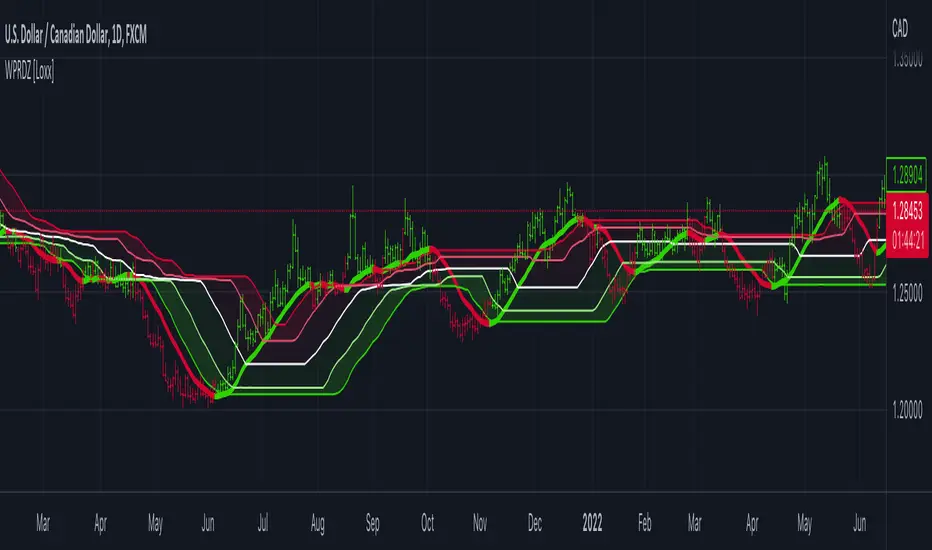
VHF-Adaptive T3 w/ Expanded Source Types [Loxx]VHF-Adaptive T3 w/ Expanded Source Types is a T3 moving average with expanded source types and adaptive period inputs using a vertical horizontal filter
What is T3?
Developed by Tim Tillson, the T3 Moving Average is considered superior to traditional moving averages as it is smoother, more responsive and thus performs better in ranging market conditions as well.
What is VHF Adaptive Cycle?
Vertical Horizontal Filter (VHF) was created by Adam White to identify trending and ranging markets. VHF measures the level of trend activity, similar to ADX DI. Vertical Horizontal Filter does not, itself, generate trading signals, but determines whether signals are taken from trend or momentum indicators. Using this trend information, one is then able to derive an average cycle length.
Included
Bar coloring
Alerts
Loxx's Expanded Source Types
