OHLC-TablesENGLISH VERSION
The command shows the opening-high-low-closing-change values of that day based on the previous value in each period.
You can set the clock in any time zone you want.
You can use the indicator by adapting it wherever you want on your screen. You can adjust its position. Top-Left-Middle Left- Bottom Left/ Top Right-Middle Right- Bottom Right.
Although it is not a command with a Buy-Sell indicator, its user-friendliness and convenience were taken into account while developing it.
The purpose of the indicator is to allow you to consider the values while focusing not only on the chart you are watching.
Pesquisar nos scripts por "OHLC"

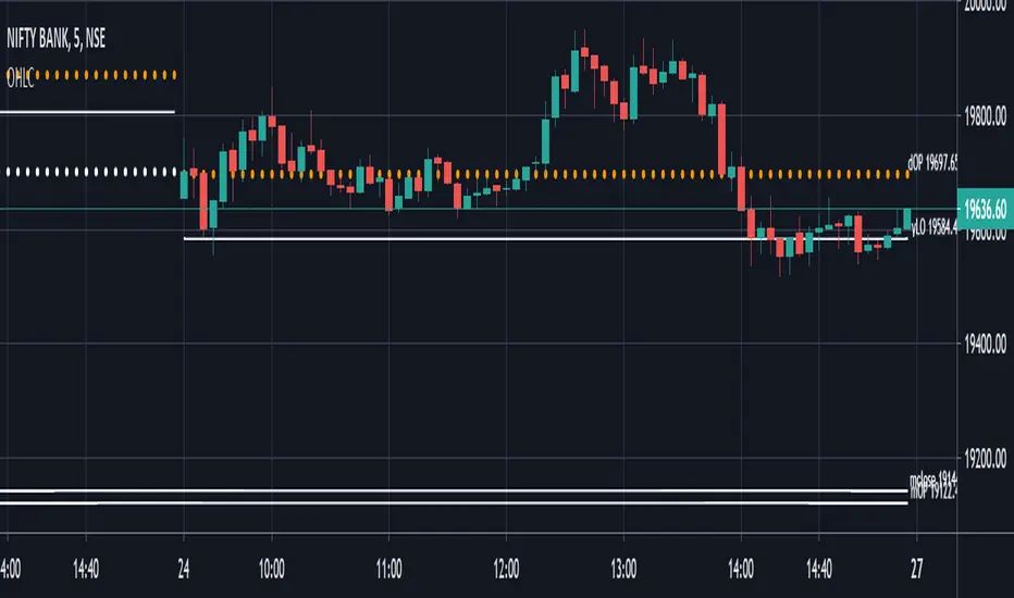
OHLC - Hourly, Daily,Weekly,Monthly with LabelsOpen, High, Low , close with Labels -- These are professional levels to watch out for active trading
dOP - Day open price
yCL - Yesterday's close Price
yHI - Yesterday's High Price
yLO -- Yesterday's Low Price
OHLC/GAP/EMA/VWAP all in oneThis script will plot the current open and previous high low and close. The overnight gap between the current open and the previous close is highlighted. Also included is the 10 EMA, 20 EMA and the VWAP. This is good for people who are limited on the amount of indicators they can use.

MA CandlesOHLC calculated with a moving average.
You can replace sma with anything. EMA, Hull, sma(sma(sma(sma(close, etc.
You could also make it look clean like Heikin Ashi candlesticks if you include min/max for low/high wicks on candles.

OHLC Volatility Estimators by @Xel_arjonaDISCLAIMER:
The Following indicator/code IS NOT intended to be a formal investment advice or recommendation by the author, nor should be construed as such. Users will be fully responsible by their use regarding their own trading vehicles/assets.
The embedded code and ideas within this work are FREELY AND PUBLICLY available on the Web for NON LUCRATIVE ACTIVITIES and must remain as is by Creative-Commons as TradingView's regulations. Any use, copy or re-use of this code should mention it's origin as it's authorship.
WARNING NOTICE!
THE INCLUDED FUNCTION MUST BE CONSIDERED AS DEBUGING CODE The models included in the function have been taken from openly sources on the web so they could have some errors as in the calculation scheme and/or in it's programatic scheme. Debugging are welcome.
WHAT'S THIS?
Here's a full collection of candle based (compressed tick) Volatility Estimators given as a function, openly available for free, it can print IMPLIED VOLATILITY by an external symbol ticker like INDEX:VIX.
Models included in the volatility calculation function:
CLOSE TO CLOSE: This is the classic estimator by rule, sometimes referred as HISTORICAL VOLATILITY and is the must common, accepted and widely used out there. Is based on traditional Standard Deviation method derived from the logarithm return of current close from yesterday's.
ELASTIC WEIGHTED MOVING AVERAGE: This estimator has been used by RiskMetriks®. It's calculation is based on an ElasticWeightedMovingAverage Standard Deviation method derived from the logarithm return of current close from yesterday's. It can be viewed or named as an EXPONENTIAL HISTORICAL VOLATILITY model.
PARKINSON'S: The Parkinson number, or High Low Range Volatility, developed by the physicist, Michael Parkinson, in 1980 aims to estimate the Volatility of returns for a random walk using the high and low in any particular period. IVolatility.com calculates daily Parkinson values. Prices are observed on a fixed time interval. n=10, 20, 30, 60, 90, 120, 150, 180 days.
ROGERS-SATCHELL: The Rogers-Satchell function is a volatility estimator that outperforms other estimators when the underlying follows a Geometric Brownian Motion (GBM) with a drift (historical data mean returns different from zero). As a result, it provides a better volatility estimation when the underlying is trending. However, this Rogers-Satchell estimator does not account for jumps in price (Gaps). It assumes no opening jump. The function uses the open, close, high, and low price series in its calculation and it has only one parameter, which is the period to use to estimate the volatility.
YANG-ZHANG: Yang and Zhang were the first to derive an historical volatility estimator that has a minimum estimation error, is independent of the drift, and independent of opening gaps. This estimator is maximally 14 times more efficient than the close-to-close estimator.
LOGARITHMIC GARMAN-KLASS: The former is a pinescript transcript of the model defined as in iVolatility . The metric used is a combination of the overnight, high/low and open/close range. Such a volatility metric is a more efficient measure of the degree of volatility during a given day. This metric is always positive.


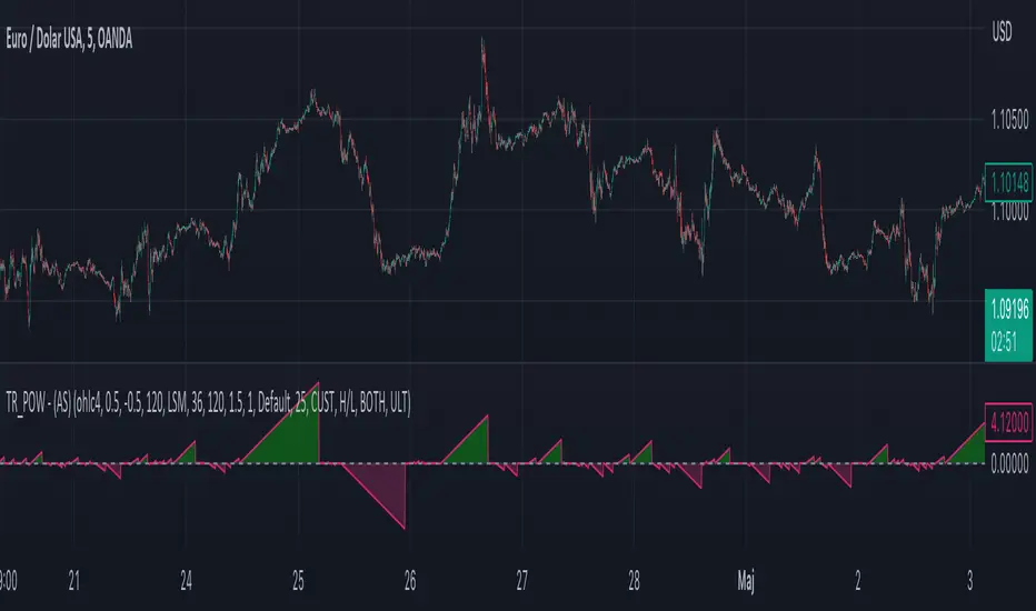
Moving Average - TREND POWER v1.1- (AS)0)NOTE:
This is first version of this indicator. It's way more complicated than it should be. Check out Moving Average-TREND POWER v2.1-(AS), its waaaaay less complicated and might be better.Enjoy...
1)INTRODUCTION/MAIN IDEA:
In simpliest form this script is a trend indicator that rises if Moving average if below price or falling if above and going back to zero if there is a crossover with a price. To use this indicator you will have to adjust settings of MAs and choose conditions for calculation.
While using the indicator we might have to define CROSS types or which MAs to use. List of what cross types are defined in the script and Conditiones to choose from.The list will be below.
2) COMPOSITION:
-MA1 can be defined by user in settings, possible types: SMA, EMA, RMA, HMA, TEMA, DEMA, LSMA, WMA.
-MA2 is always ALMA
3) OVERLAY:
Default is false but if you want to see MA1/2 on chart you can change code to true and then turn on overlay in settings. Most plot settings are avalible only in OV=false.
if OV=true possible plots ->MA1/2, plotshape when choosen cross type
if OV=false -> main indicator,TSHs,Cross counter
4)PRESETS :
Indicator has three modes that can be selected in settings. First two are presets and do not require selecting conditions as they set be default.
-SIMPLE - most basic
-ABSOLUTE - shows only positive values when market is trending or zero when in range
-CUSTOM - main and the most advanced form that will require setting conditions to use in calculating trend
4.1)SIMPLE – this is the most basic form of conditions that uses only First MA. If MA1 is below selected source (High/Low(High for Uptrend and Low for DNtrend or OHLC4) on every bar value rises by 0.02. if it above Low or OHLC4 it falls by 0.02 with every bar. If there is a cross of MA with price value is zero. This preset uses CROSS_1_ULT(list of all cross types below)
4.2) ABSOLUTE – does not show direction of the trend unlike others and uses both MA1 and MA2. Uses CROSS type 123_ULT
4.3) CUSTOM – here we define conditions manually. This mode is defined in parts (5-8 of description)
5)SETTINGS:
SOURCE/OVERLAY(line1) – select source of calculation form MA1/MA2, select for overlay true (look point 3)
TRESHOLDS(line2). – set upper and lower THS, turn TSHs on/off
MA1(line3) – Length/type of MA/Offset(only if MA type is LSM)
MA2(line4) – length/offset/sigma -(remember to set ma in the way that in Uptrend MA2MA1 in DNtrend)
Use faster MA types for short term trends and slower types / bigger periods for longer term trends, defval MA1/2 settings
are pretty much random so using them is not recomended.
CROSSshape(line5) – choose which cross type you want to plot on chart(only in OV=true) or what type you want to use in counting via for loops,
CROSScount(line6) – set lookback for type of cross choosen above
BOOLs in lines 5 and 6 - plotshape if OV=true/plot CROSScount histogram (if OV=false)
Lines 7 and 8 – PRESET we want to use /SRC for calculation of indicator/are conditions described below/which MAs to use/Condition for
reducing value t 0 - (if PRESET is ABSOLUTE or SIMPLE only SRC should be set(Line 8 does not matter if not CUSTOM))
5)SOURCE for CONDS:
Here you can choose between H/L and OHLC. If H/L value grow when MAlow. If OHLC MAOHLC. H/L is set by default and recommended. This can be selected for all presets not only CUSTOM
6)CROSS types LIST:
“1 means MA1, 2 is MA2 and 3 I cross of MA1/MA2. L stands for low and H for high so for example 2H means cross of MA2 and high”
NAME -DEFINITION Number of possible crosses
1L - cross of MA1 and low 1
1H - cross of MA1 and high 1
1HL - cross of MA1 and low or MA1 and high 2 -1L/1H
2L - cross of MA2 and low 1
2H - cross of MA2 and high 1
2HL - cross of MA2 and low or MA1 and high 2 -2L/2H
12L - cross of MA1 and low or MA2 and low 2 -1L/2L
12H - cross of MA1 and high or MA2 and high 2 -1H/2H
12HL - MA1/2 and high/low 4 -1H/1L/2H/2L
3 -cross of MA1 and MA2 1
123HL -crosses from 12HL or 3 5 -12HL/3
1_ULT - cross of MA1 with any of price sources(close,low,high,ohlc4 etc…)
2_ULT - cross of MA2 with any of price sources(close,low,high,ohlc4 etc…)
123_ULT – all crosses possible of MA1/2 (all of the above so a lot)
7)CRS CONDS:
“conditions to reduce value back to zero”
>/< - 0 if indicator shows Uptrend and there’s a cross with high of selected MA or 0 if in DNtrend and cross with low. Better for UP/DN trend detection
ALL – 0 if cross of MA with high or low no matter the trend, better for detecting consolidation
ULT – if any cross of selected MA, most crosses so goes to 0 most often
8)MA selection and CONDS:
-MA1: only MA1 is used,if MA1 below price value grows and the other way around
MA1price =-0.02
-MA2 – only MA2 is used, same conditions as MA1 but using MA2
MA2price =-0.02
-BOTH – MA1 and MA2 used, grows when MA1 if below, grows faster if MA1 and MA2 are below and fastest when MA1 and MA2 are below and MA2price=-0.02
-MA1 and MA2 >price=-0.03
-MA1 and MA2 ?price and MA2>MA1=-0.04
9)CONDITIONS SELECTION SUMMARRY:
So when CUSTOM we choose :
1)SOURCE – H/L or OHLC
2)MAs – MA1/MA2/BOTH
3)CRS CONDS (>/<,ALL,ULT)
So for example...
if we take MA1 and ALL value will go to zero if 1HL
if MA1 and >/< - 0 if 1L or 1H (depending if value is positive or negative).(1L or 1H)
If ALL and BOTH zero when 12HL
If BOTH and ULT value goes back to zero if Theres any cross of MA1/MA2 with price or cross of MA1 and MA2.(123_ULT)
If >/< and BOTH – 0 if 12L in DNtrend or 12H if UPtrend
10) OTHERS
-script was created on EURUSD 5M and wasn't tested on different markets
-default values of MA1/MA2 aren't optimalized so do not
-There might be a logical error in the script so let me know if you find it (most probably in 'BOTH')
-thanks to @AlifeToMake for help
-if you have any ideas to improve let me know
-there are also tooltips to help
Volume Sampled Supertrend [BackQuant]Volume Sampled Supertrend
A Supertrend that runs on a volume sampled price series instead of fixed time. New synthetic bars are only created after sufficient traded activity, which filters out low participation noise and makes the trend much easier to read and model.
Original Script Link
This indicator is built on top of my volume sampling engine. See the base implementation here:
Why Volume Sampling
Traditional charts print a bar every N minutes regardless of how active the tape is. During quiet periods you accumulate many small, low information bars that add noise and whipsaws to downstream signals.
Volume sampling replaces the clock with participation. A new synthetic bar is created only when a pre-set amount of volume accumulates (or, in Dollar Bars mode, when pricevolume reaches a dollar threshold). The result is a non-uniform time series that stretches in busy regimes and compresses in quiet regimes. This naturally:
filters dead time by skipping low volume chop;
standardizes the information content per bar, improving comparability across regimes;
stabilizes volatility estimates used inside banded indicators;
gives trend and breakout logic cleaner state transitions with fewer micro flips.
What this tool does
It builds a synthetic OHLCV stream from volume based buckets and then applies a Supertrend to that synthetic price. You are effectively running Supertrend on a participation clock rather than a wall clock.
Core Features
Sampling Engine - Choose Volume buckets or Dollar Bars . Thresholds can be dynamic from a rolling mean or median, or fixed by the user.
Synthetic Candles - Plots the volume sampled OHLC candles so you can visually compare against regular time candles.
Supertrend on Synthetic Price - ATR bands and direction are computed on the sampled series, not on time bars.
Adaptive Coloring - Candle colors can reflect side, intensity by volume, or a neutral scheme.
Research Panels - Table shows total samples, current bucket fill, threshold, bars-per-sample, and synthetic return stats.
Alerts - Long and Short triggers on Supertrend direction flips for the synthetic series.
How it works
Sampling
Pick Sampling Method = Volume or Dollar Bars.
Set the dynamic threshold via Rolling Lookback and Filter (Mean or Median), or enable Use Fixed and type a constant.
The script accumulates volume (or pricevolume) each time bar. When the bucket reaches the threshold, it finalizes one or more synthetic candles and resets accumulation.
Each synthetic candle stores its own OHLCV and is appended to the synthetic series used for all downstream logic.
Supertrend on the sampled stream
Choose Supertrend Source (Open, High, Low, Close, HLC3, HL2, OHLC4, HLCC4) derived from the synthetic candle.
Compute ATR over the synthetic series with ATR Period , then form upperBand = src + factorATR and lowerBand = src - factorATR .
Apply classic trailing band and direction rules to produce Supertrend and trend state.
Because bars only come when there is sufficient participation, band touches and flips tend to align with meaningful pushes, not idle prints.
Reading the display
Synthetic Volume Bars - The non-uniform candles that represent equal information buckets. Expect more candles during active sessions and fewer during lulls.
Volume Sampled Supertrend - The main line. Green when Trend is 1, red when Trend is -1.
Markers - Small dots appear when a new synthetic sample is created, useful for aligning activity cycles.
Time Bars Overlay (optional) - Plot regular time candles to compare how the synthetic stream compresses quiet chop.
Settings you will use most
Data Settings
Sampling Method - Volume or Dollar Bars.
Rolling Lookback and Filter - Controls the dynamic threshold. Median is robust to outliers, Mean is smoother.
Use Fixed and Fixed Threshold - Force a constant bucket size for consistent sampling across regimes.
Max Stored Samples - Ring buffer limit for performance.
Indicator Settings
SMA over last N samples - A moving average computed on the synthetic close series. Can be hidden for a cleaner layout.
Supertrend Source - Price field from the synthetic candle.
ATR Period and Factor - Standard Supertrend controls applied on the synthetic series.
Visuals and UI
Show Synthetic Bars - Turn synthetic candles on or off.
Candle Color Mode - Green/Red, Volume Intensity, Neutral, or Adaptive.
Mark new samples - Puts a dot when a bucket closes.
Show Time Bars - Overlay regular candles for comparison.
Paint candles according to Trend - Colors chart candles using current synthetic Supertrend direction.
Line Width , Colors , and Stats Table toggles.
Some workflow notes:
Trend Following
Set Sampling Method = Volume, Filter = Median, and a reasonable Rolling Lookback so busy regimes produce more samples.
Trade in the direction of the Volume Sampled Supertrend. Because flips require real participation, you tend to avoid micro whipsaws seen on time bars.
Use the synthetic SMA as a bias rail and trailing reference for partials or re-entries.
Breakout and Continuation
Watch for rapid clustering of new sample markers and a clean flip of the synthetic Supertrend.
The compression of quiet time and expansion in busy bursts often makes breakouts more legible than on uniform time charts.
Mean Reversion
In instruments that oscillate, faded moves against the synthetic Supertrend are easier to time when the bucket cadence slows and Supertrend flattens.
Combine with the synthetic SMA and return statistics in the table for sizing and expectation setting.
Stats table (top right)
Method and Total Samples - Sampling regime and current synthetic history length.
Current Vol or Dollar and Threshold - Live bucket fill versus the trigger.
Bars in Bucket and Avg Bars per Sample - How much time data each synthetic bar tends to compress.
Avg Return and Return StdDev - Simple research metrics over synthetic close-to-close changes.
Why this reduces noise
Time based bars treat a 5 minute print with 1 percent of average participation the same as one with 300 percent. Volume sampling equalizes bar information content. By advancing the bar only when sufficient activity occurs, you skip low quality intervals that add variance but little signal. For banded systems like Supertrend, this often means fewer false flips and cleaner runs.
Notes and tips
Use Dollar Bars on assets where nominal price varies widely over time or across symbols.
Median filter can resist single burst outliers when setting dynamic thresholds.
If you need a stable research baseline, set Use Fixed and keep the threshold constant across tests.
Enable Show Time Bars occasionally to sanity check what the synthetic stream is compressing or stretching.
Link again for reference
Original Volume Based Sampling engine:
Bottom line
When you let participation set the clock, your Supertrend reacts to meaningful flow instead of idle prints. The result is a cleaner state machine, fewer micro whipsaws, and a trend read that respects when the market is actually trading.

basechartpatternsLibrary "basechartpatterns"
Library having complete chart pattern implementation
getPatternNameById(id)
Returns pattern name by id
Parameters:
id (int) : pattern id
Returns: Pattern name
method find(points, properties, dProperties, ohlcArray)
Find patterns based on array of points
Namespace types: chart.point
Parameters:
points (chart.point ) : array of chart.point objects
properties (ScanProperties type from Trendoscope/abstractchartpatterns/1) : ScanProperties object
dProperties (DrawingProperties type from Trendoscope/abstractchartpatterns/1) : DrawingProperties object
ohlcArray (OHLC type from Trendoscope/ohlc/1)
Returns: Flag indicating if the pattern is valid, Current Pattern object
method find(this, properties, dProperties, patterns, ohlcArray)
Find patterns based on the currect zigzag object but will not store them in the pattern array.
Namespace types: zg.Zigzag
Parameters:
this (Zigzag type from Trendoscope/ZigzagLite/2) : Zigzag object containing pivots
properties (ScanProperties type from Trendoscope/abstractchartpatterns/1) : ScanProperties object
dProperties (DrawingProperties type from Trendoscope/abstractchartpatterns/1) : DrawingProperties object
patterns (Pattern type from Trendoscope/abstractchartpatterns/1) : Array of Pattern objects
ohlcArray (OHLC type from Trendoscope/ohlc/1)
Returns: Flag indicating if the pattern is valid, Current Pattern object
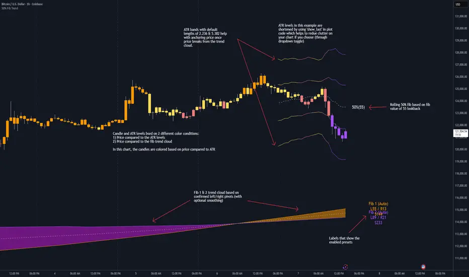
50% Fib Trend Cloud + ATR BandsThis indicator plots two structural 50% fibonacci midpoints from recent confirmed 'left/right' swings that form a *cloud* of equilibrium, then adds a rolling 50% fibonacci range midpoint based on a lookback window that's wrapped in ATR bands. Importantly, it solves a specific trading problem:
Structural midpoints (macro context) are powerful but can lag when price escapes prior ranges. Enter rolling 50% fib + ATR ➡️ which restores real-time balance & tolerance (micro context). Together they show where price is balanced structurally, where it’s balanced right now, and how much volatility to tolerate before acting.
➖➖➖
🔑 Why this is different
Most tools either draw a single midpoint (ex., daily 50%) or ATR bands around a moving average. This script fuses dual swing-based 50% midpoints (structure) + a rolling 50% with ATR (flow), so you don’t lose context when price escapes prior ranges. The cloud tells you who’s in control (fast vs. slow structure). The rolling 50% + ATR tells you how far is “too far” now.
➖➖➖
🧠 What it does (at a glance)
🔸Structural Equilibrium × 2 (Fib1/Fib2)
Two independent 50% midpoints formed from swing pivots (configurable Left/Right bars + optional smoothing). Their gap is the Midpoint Cloud = structural “fair value” zone.
🔸Rolling 50% + ATR Bands
A rolling highest/lowest window computes an always-current 50% rolling midpoint plot; ±ATR × length envelopes define a soft value area and over-stretch boundaries.
🔸Actionable Visuals
Optional fill between Fib1/Fib2, labels, and candle-overlay modes to instantly read regime (above both / below both / between).
🔸Smart Defaults
Timeframe-aware presets for L/R pivots & smoothing; full manual overrides available.
➖➖➖
⚙️ Calculations (plain-English)
🔸Pivot midpoints (Fib1 & Fib2):
1) Detect a swing using `Left/Right` bars
2) Take the swing’s high/low → compute 50%
3) (Optional) Smooth the line (SMA) to stabilize on noisy TFs
4) Repeat with a different sensitivity to get two distinct midpoints
🔸Rolling midpoint:
Highest High / Lowest Low over the last *N* bars → (HH + LL) / 2
🔸ATR levels:
`Upper = Rolling50 + ATR × Mult`, `Lower = Rolling50 − ATR × Mult`
(Typical: ATR length 14–21; Multipliers 2.236 for L1, 5.382 for L2)
➖➖➖
🤖 Auto-Configured Presets (with Manual Override)
💡Goal: make the midpoints “just work” on common timeframes while still letting you dial them in.
💡How Auto Presets work
When Auto Presets = ON, the script picks sensible L/R/S (Left bars / Right bars / Smoothing) for Fib Trend 1 and Fib Trend 2 based on chart timeframe.
🔸Fib 1 (fast) emphasizes *micro-structure* for quicker bias shifts.
🔸Fib 2 (slow) emphasizes *macro-structure* for anchor/bias context.
These defaults keep Fib 1 responsive without jitter and Fib 2 stable without lag.
➡️ Turn Auto Presets = OFF to take full control with the manual inputs described below.
➖➖➖
🛠 Manual Fib Midpoint Settings (when Auto = OFF)
💡Each midpoint uses three knobs:
🔸Pivot Left (L): bars to the left that must be lower/higher to qualify a swing
🔸Pivot Right (R): bars to the right that must be lower/higher to confirm the swing
🔸Smoothing (S): SMA period applied to the raw 50% midpoint (stabilizes noise)
5-Minute optimized defaults
🔸Fib Trend 1: `L21 / R5 / S55` → responsive local structure (entries/exits, re-balancing zones)
🔸Fib Trend 2: `L55 / R13 / S89` → broader structure (trend context, anchors/stops)
Timeframe guidance
🔸1m–3m: may feel a touch laggy → consider ~`L13 / R3 / S34`
🔸15m–1h: defaults remain strong → optionally ~`L34 / R8 / S89`
🔸4h+ : increase span for stability → `L89–144 / R13–21 / S144–233`
➡️ Rule of thumb: shorter L/R = faster detection, longer S = smoother line. Tune until Fib 1 captures the “active swing” and Fib 2 captures the “dominant swing” without whipsaw.
➖➖➖
🎛 Inputs (quick reference)
🔸Fib Trend 1/2: Source (High/Low/Close), Left/Right bars, Smoothing length, Show/Hide, Cloud fill toggle
🔸Rolling 50%: Lookback length, Price basis (Wicks/Close/HLC3/OHLC4), Plot scope (Full / Last N / None)
🔸ATR Bands: ATR length, Multipliers (L1/L2), Plot scope, Line width/colors
🔸Overlay & Labels: Candle overlay mode, Label padding/size, 50% centerline toggle, Plot widths
➖➖➖
🖍️ Candle Coloring & Overlay Modes
💡Purpose: make trend instantly visible on the candles and ATR levels.
1) Color Logic (dropdown)
🔸 Fib Midpoints — Colors by position of price vs. Fib 1 & Fib 2
🔸ATR Zones — Colors by which ATR zone price is in relative to the Rolling 50%
➡️ Price Reference: Choose the input used for the decision (Close, HL2, OHLC3, OHLC4).
➡️Tip: Close is crisp; HL2/OHLC variants are smoother.
2) Overlay Style (dropdown)
🔸 None — No visual change to candles
🔸 Bar Color — Uses `barcolor()` to tint built-in candles (this takes into account your Trading View settings, for instance if you have wicks set to white, they will show up as white with this setting)
🔸 PlotCandles — Draws unified custom candles (body, wick, border) with the same color for maximum clarity
💡Practical use
🔸 Pick Fib Midpoints to read structural bias at a glance (above/below/between the cloud).
🔸 Pick ATR Zones to read value vs. stretch around the Rolling 50% (mean-reversion vs. trend extension).
➖➖➖
📘 How to use
A) Trend confirmation
- Strong bullish bias when price holds above both structural mids; strong bearish when below both.
- Use the Rolling 50% + ATR as a dynamic re-entry zone: pullbacks that respect ATR(L1) often continue the prevailing trend.
B) Transition / mean reversion
- Inside the Cloud (between Fib1 & Fib2) treat behavior as neutralization/re-balancing; range tactics tend to outperform momentum plays.
- In ranges, fades near ±ATR around the rolling 50% can mark short-term edges.
C) Breakout context
- When price leaves the Cloud, the Rolling 50% keeps you anchored so price never feels “floating.” A clean hold outside ATR(L1/L2) suggests regime strength; quick re-entries hint at traps.
➖➖➖
🖼 Chart examples
➡️ Each snapshot shows how the Cloud (structure) and the Rolling 50% + ATR (flow) work together.
1) 1-Minute Downtrend – Cloud as Dynamic Ceiling
- The Cloud slopes down; pullbacks repeatedly fail under the Cloud’s underside.
- Rolling 50% (dashed mid) + ATR(L1) act as a reversion band: rallies stall near upper ATR and rotate lower.
2) 15-Minute Persistent Drift – Structure Guides, Flow Times Entries
- Long drift lower with Cloud overhead.
- Consolidations near the rolling mid resolve in the trend direction; ATR bands frame risk on each attempt.
3) 15-Minute Uptrend (BTC) – From Cloud Escape to Value Stair-Step
- After escaping the prior Cloud, rolling 50% + ATR establish a new higher value area.
- Pullbacks into ATR(L1) produce orderly stair-steps; Cloud remains supportive on deeper dips
4) 5-Minute BTC – Pullback to Value then Rotate
- Strong leg up; retrace tags lower ATR band and rotates back toward the rolling mid.
- Labels (Fib1/Fib2) make the structural context explicit for decision-making.
➖➖➖
🧪 Starter presets
- Intraday (5–15m): Fib1 ~ L21/R5 (smooth 5), Fib2 ~ L55/R13 (smooth 9) • Rolling = 55 • ATR = 14 • L1 = 2.5x, L2 = 5.0x
- Scalping: Shorten lookbacks & smoothing; keep ATR multipliers similar, or tighten L1.
- Swing: Lengthen all lookbacks; consider ATR length 21–28.
➖➖➖
🏁Final Word
This script is not just a visual tool, it’s a complete trend and structure framework. Whether you're looking for clean trend alignment, dynamic support/resistance, or early warning signs of a reversal, this system is tuned to help you react with confidence — not hindsight.
Rembember, no single indicator should be used in isolation. For best results, combine it with price action analysis, higher-timeframe context, and complementary tools like trendlines, moving averages etc Use it as part of a well-rounded trading approach to confirm setups — not to define them alone.
---
💡Turn logic into clarity. Structure into trades. And uncertainty into confidence.
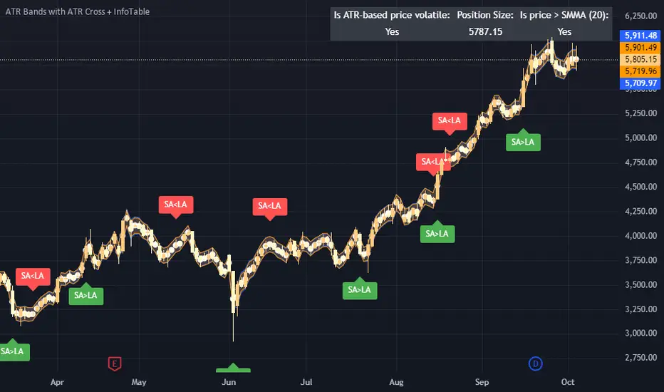
ATR Bands with ATR Cross + InfoTableOverview
This Pine Script™ indicator is designed to enhance traders' ability to analyze market volatility, trend direction, and position sizing directly on their TradingView charts. By plotting Average True Range (ATR) bands anchored at the OHLC4 price, displaying crossover labels, and providing a comprehensive information table, this tool offers a multifaceted approach to technical analysis.
Key Features:
ATR Bands Anchored at OHLC4: Visual representation of short-term and long-term volatility bands centered around the average price.
OHLC4 Dotted Line: A dotted line representing the average of Open, High, Low, and Close prices.
ATR Cross Labels: Visual cues indicating when short-term volatility exceeds long-term volatility and vice versa.
Information Table: Displays real-time data on market volatility, calculated position size based on risk parameters, and trend direction relative to the 20-period Smoothed Moving Average (SMMA).
Purpose
The primary purpose of this indicator is to:
Assess Market Volatility: By comparing short-term and long-term ATR values, traders can gauge the current volatility environment.
Determine Optimal Position Sizing: A calculated position size based on user-defined risk parameters helps in effective risk management.
Identify Trend Direction: Comparing the current price to the 20-period SMMA assists in determining the prevailing market trend.
Enhance Decision-Making: Visual cues and real-time data enable traders to make informed trading decisions with greater confidence.
How It Works
1. ATR Bands Anchored at OHLC4
Average True Range (ATR) Calculations
Short-Term ATR (SA): Calculated over a 9-period using ta.atr(9).
Long-Term ATR (LA): Calculated over a 21-period using ta.atr(21).
Plotting the Bands
OHLC4 Dotted Line: Plotted using small circles to simulate a dotted line due to Pine Script limitations.
ATR(9) Bands: Plotted in blue with semi-transparent shading.
ATR(21) Bands: Plotted in orange with semi-transparent shading.
Overlap: Bands can overlap, providing visual insights into changes in volatility.
2. ATR Cross Labels
Crossover Detection:
SA > LA: Indicates increasing short-term volatility.
Detected using ta.crossover(SA, LA).
A green upward label "SA>LA" is plotted below the bar.
SA < LA: Indicates decreasing short-term volatility.
Detected using ta.crossunder(SA, LA).
A red downward label "SA LA, then the market is considered volatile.
Display: Shows "Yes" or "No" based on the comparison.
b. Position Size Calculation
Risk Total Amount: User-defined input representing the total capital at risk.
Risk per 1 Stock: User-defined input representing the risk associated with one unit of the asset.
Purpose: Helps traders determine the appropriate position size based on their risk tolerance and current market volatility.
c. Is Price > 20 SMMA?
SMMA Calculation:
Calculated using a 20-period Smoothed Moving Average with ta.rma(close, 20).
Logic: If the current close price is above the SMMA, the trend is considered upward.
Display: Shows "Yes" or "No" based on the comparison.
How to Use
Step 1: Add the Indicator to Your Chart
Copy the Script: Copy the entire Pine Script code into the TradingView Pine Editor.
Save and Apply: Save the script and click "Add to Chart."
Step 2: Configure Inputs
Risk Parameters: Adjust the "Risk Total Amount" and "Risk per 1 Stock" in the indicator settings to match your personal risk management strategy.
Step 3: Interpret the Visuals
ATR Bands
Width of Bands: Wider bands indicate higher volatility; narrower bands indicate lower volatility.
Band Overlap: Pay attention to areas where the blue and orange bands diverge or converge.
OHLC4 Dotted Line
Serves as a central reference point for the ATR bands.
Helps visualize the average price around which volatility is measured.
ATR Cross Labels
"SA>LA" Label:
Indicates short-term volatility is increasing relative to long-term volatility.
May signal potential breakout or trend acceleration.
"SA 20 SMMA?
Use this to confirm trend direction before entering or exiting trades.
Practical Example
Imagine you are analyzing a stock and notice the following:
ATR(9) Crosses Above ATR(21):
A green "SA>LA" label appears.
The info table shows "Yes" for "Is ATR-based price volatile."
Position Size:
Based on your risk parameters, the position size is calculated.
Price Above 20 SMMA:
The info table shows "Yes" for "Is price > 20 SMMA."
Interpretation:
The market is experiencing increasing short-term volatility.
The trend is upward, as the price is above the 20 SMMA.
You may consider entering a long position, using the calculated position size to manage risk.
Customization
Colors and Transparency:
Adjust the colors of the bands and labels to suit your preferences.
Risk Parameters:
Modify the default values for risk amounts in the inputs.
Moving Average Period:
Change the SMMA period if desired.
Limitations and Considerations
Lagging Indicators: ATR and SMMA are lagging indicators and may not predict future price movements.
Market Conditions: The effectiveness of this indicator may vary across different assets and market conditions.
Risk of Overfitting: Relying solely on this indicator without considering other factors may lead to suboptimal trading decisions.
Conclusion
This indicator combines essential elements of technical analysis to provide a comprehensive tool for traders. By visualizing ATR bands anchored at the OHLC4, indicating volatility crossovers, and providing real-time data on position sizing and trend direction, it aids in making informed trading decisions.
Whether you're a novice trader looking to understand market volatility or an experienced trader seeking to refine your strategy, this indicator offers valuable insights directly on your TradingView charts.
Code Summary
The script is written in Pine Script™ version 5 and includes:
Calculations for OHLC4, ATRs, Bands, SMMA:
Uses built-in functions like ta.atr() and ta.rma() for calculations.
Plotting Functions:
plotshape() for the OHLC4 dotted line.
plot() and fill() for the ATR bands.
Crossover Detection:
ta.crossover() and ta.crossunder() for detecting ATR crosses.
Labeling Crossovers:
label.new() to place informative labels on the chart.
Information Table Creation:
table.new() to create the table.
table.cell() to populate it with data.
Acknowledgments
ATR and SMMA Concepts: Built upon standard technical analysis concepts widely used in trading.
Pine Script™: Leveraged the capabilities of Pine Script™ version 5 for advanced charting and analysis.
Note: Always test any indicator thoroughly and consider combining it with other forms of analysis before making trading decisions. Trading involves risk, and past performance is not indicative of future results.
Happy Trading!
divergingchartpatternLibrary "divergingchartpattern"
Library having implementation of converging chart patterns
getPatternNameByType(patternType)
Returns pattern name based on type
Parameters:
patternType (int) : integer value representing pattern type
Returns: string name of the pattern
method find(this, sProperties, dProperties, patterns, ohlcArray)
find converging patterns for given zigzag
Namespace types: zg.Zigzag
Parameters:
this (Zigzag type from Trendoscope/ZigzagLite/2) : Current zigzag Object
sProperties (ScanProperties) : ScanProperties Object
dProperties (DrawingProperties type from Trendoscope/abstractchartpatterns/5) : DrawingProperties Object
patterns (array type from Trendoscope/abstractchartpatterns/5) : array of existing patterns to check for duplicates
ohlcArray (array type from Trendoscope/ohlc/1) : array of OHLC values for historical reference
Returns: string name of the pattern
ScanProperties
Object containing properties for pattern scanning
Fields:
baseProperties (ScanProperties type from Trendoscope/abstractchartpatterns/5) : Object of Base Scan Properties
convergingDistanceMultiplier (series float)
convergingpatternsLibrary "convergingpatterns"
Library having implementation of converging chart patterns
getPatternNameByType(patternType)
Returns pattern name based on type
Parameters:
patternType (int) : integer value representing pattern type
Returns: string name of the pattern
method find(this, sProperties, dProperties, patterns, ohlcArray)
find converging patterns for given zigzag
Namespace types: zg.Zigzag
Parameters:
this (Zigzag type from Trendoscope/ZigzagLite/2) : Current zigzag Object
sProperties (ScanProperties) : ScanProperties Object
dProperties (DrawingProperties type from Trendoscope/abstractchartpatterns/5) : DrawingProperties Object
patterns (array type from Trendoscope/abstractchartpatterns/5) : array of existing patterns to check for duplicates
ohlcArray (array type from Trendoscope/ohlc/1) : array of OHLC values for historical reference
Returns: string name of the pattern
ScanProperties
Object containing properties for pattern scanning
Fields:
baseProperties (ScanProperties type from Trendoscope/abstractchartpatterns/5) : Object of Base Scan Properties
convergingDistanceMultiplier (series float) : when multiplied with pattern size gets the max number of bars within which the pattern should converge
abstractchartpatternsLibrary "abstractchartpatterns"
Library having abstract types and methods for chart pattern implementations
checkBarRatio(p1, p2, p3, properties)
checks if three zigzag pivot points are having uniform bar ratios
Parameters:
p1 (chart.point) : First pivot point
p2 (chart.point) : Second pivot point
p3 (chart.point) : Third pivot point
properties (ScanProperties)
Returns: true if points are having uniform bar ratio
getRatioDiff(p1, p2, p3)
gets ratio difference between 3 pivot combinations
Parameters:
p1 (chart.point)
p2 (chart.point)
p3 (chart.point)
Returns: returns the ratio difference between pivot2/pivot1 ratio and pivot3/pivot2 ratio
method inspect(points, stratingBar, endingBar, direction, ohlcArray)
Creates a trend line between 2 or 3 points and validates and selects best combination
Namespace types: chart.point
Parameters:
points (chart.point ) : Array of chart.point objects used for drawing trend line
stratingBar (int) : starting bar of the trend line
endingBar (int) : ending bar of the trend line
direction (float) : direction of the last pivot. Tells whether the line is joining upper pivots or the lower pivots
ohlcArray (OHLC type from Trendoscope/ohlc/1) : Array of OHLC values
Returns: boolean flag indicating if the trend line is valid and the trend line object as tuple
method draw(this)
draws pattern on the chart
Namespace types: Pattern
Parameters:
this (Pattern) : Pattern object that needs to be drawn
Returns: Current Pattern object
method erase(this)
erase the given pattern on the chart
Namespace types: Pattern
Parameters:
this (Pattern) : Pattern object that needs to be erased
Returns: Current Pattern object
method push(this, p, maxItems)
push Pattern object to the array by keeping maxItems limit
Namespace types: Pattern
Parameters:
this (Pattern ) : array of Pattern objects
p (Pattern) : Pattern object to be added to array
@oaram maxItems Max number of items the array can hold
maxItems (int)
Returns: Current Pattern array
method deepcopy(this)
Perform deep copy of a chart point array
Namespace types: chart.point
Parameters:
this (chart.point ) : array of chart.point objects
Returns: deep copy array
DrawingProperties
Object containing properties for pattern drawing
Fields:
patternLineWidth (series int) : Line width of the pattern trend lines
showZigzag (series bool) : show zigzag associated with pattern
zigzagLineWidth (series int) : line width of the zigzag lines. Used only when showZigzag is set to true
zigzagLineColor (series color) : color of the zigzag lines. Used only when showZigzag is set to true
showPatternLabel (series bool) : display pattern label containing the name
patternLabelSize (series string) : size of the pattern label. Used only when showPatternLabel is set to true
showPivotLabels (series bool) : Display pivot labels of the patterns marking 1-6
pivotLabelSize (series string) : size of the pivot label. Used only when showPivotLabels is set to true
pivotLabelColor (series color) : color of the pivot label outline. chart.bg_color or chart.fg_color are the appropriate values.
deleteOnPop (series bool) : delete the pattern when popping out from the array of Patterns.
Pattern
Object containing Individual Pattern data
Fields:
points (chart.point )
originalPoints (chart.point )
trendLine1 (Line type from Trendoscope/LineWrapper/1) : First trend line joining pivots 1, 3, 5
trendLine2 (Line type from Trendoscope/LineWrapper/1) : Second trend line joining pivots 2, 4 (, 6)
properties (DrawingProperties) : DrawingProperties Object carrying common properties
patternColor (series color) : Individual pattern color. Lines and labels will be using this color.
ratioDiff (series float) : Difference between trendLine1 and trendLine2 ratios
zigzagLine (series polyline) : Internal zigzag line drawing Object
pivotLabels (label ) : array containning Pivot labels
patternLabel (series label) : pattern label Object
patternType (series int) : integer representing the pattern type
patternName (series string) : Type of pattern in string
ScanProperties
Object containing properties for pattern scanning
Fields:
offset (series int) : Zigzag pivot offset. Set it to 1 for non repainting scan.
numberOfPivots (series int) : Number of pivots to be used in pattern search. Can be either 5 or 6
errorRatio (series float) : Error Threshold to be considered for comparing the slope of lines
flatRatio (series float) : Retracement ratio threshold used to determine if the lines are flat
checkBarRatio (series bool) : Also check bar ratio are within the limits while scanning the patterns
barRatioLimit (series float) : Bar ratio limit used for checking the bars. Used only when checkBarRatio is set to true
avoidOverlap (series bool) : avoid overlapping patterns.
allowedPatterns (bool ) : array of bool encoding the allowed pattern types.
allowedLastPivotDirections (int ) : array of int representing allowed last pivot direction for each pattern types
themeColors (color ) : color array of themes to be used.

Volume Delta Volume Signals by Claudio [hapharmonic]// This Pine Script™ code is subject to the terms of the Mozilla Public License 2.0 at mozilla.org
// © hapharmonic
//@version=6
FV = format.volume
FP = format.percent
indicator('Volume Delta Volume Signals by Claudio ', format = FV, max_bars_back = 4999, max_labels_count = 500)
//------------------------------------------
// Settings |
//------------------------------------------
bool usecandle = input.bool(true, title = 'Volume on Candles',display=display.none)
color C_Up = input.color(#12cef8, title = 'Volume Buy', inline = ' ', group = 'Style')
color C_Down = input.color(#fe3f00, title = 'Volume Sell', inline = ' ', group = 'Style')
// ✅ Nueva entrada para colores de señales
color buySignalColor = input.color(color.new(color.green, 0), "Buy Signal Color", group = "Signals")
color sellSignalColor = input.color(color.new(color.red, 0), "Sell Signal Color", group = "Signals")
string P_ = input.string(position.top_right,"Position",options = ,
group = "Style",display=display.none)
string sL = input.string(size.small , 'Size Label', options = , group = 'Style',display=display.none)
string sT = input.string(size.normal, 'Size Table', options = , group = 'Style',display=display.none)
bool Label = input.bool(false, inline = 'l')
History = input.bool(true, inline = 'l')
// Inputs for EMA lengths and volume confirmation
bool MAV = input.bool(true, title = 'EMA', group = 'EMA')
string volumeOption = input.string('Use Volume Confirmation', title = 'Volume Option', options = , group = 'EMA',display=display.none)
bool useVolumeConfirmation = volumeOption == 'none' ? false : true
int emaFastLength = input(12, title = 'Fast EMA Length', group = 'EMA',display=display.none)
int emaSlowLength = input(26, title = 'Slow EMA Length', group = 'EMA',display=display.none)
int volumeConfirmationLength = input(6, title = 'Volume Confirmation Length', group = 'EMA',display=display.none)
string alert_freq = input.string(alert.freq_once_per_bar_close, title="Alert Frequency",
options= ,group = "EMA",
tooltip="If you choose once_per_bar, you will receive immediate notifications (but this may cause interference or indicator repainting).
\n However, if you choose once_per_bar_close, it will wait for the candle to confirm the signal before notifying.",display=display.none)
//------------------------------------------
// UDT_identifier |
//------------------------------------------
type OHLCV
float O = open
float H = high
float L = low
float C = close
float V = volume
type VolumeData
float buyVol
float sellVol
float pcBuy
float pcSell
bool isBuyGreater
float higherVol
float lowerVol
color higherCol
color lowerCol
//------------------------------------------
// Calculate volumes and percentages |
//------------------------------------------
calcVolumes(OHLCV ohlcv) =>
var VolumeData data = VolumeData.new()
data.buyVol := ohlcv.V * (ohlcv.C - ohlcv.L) / (ohlcv.H - ohlcv.L)
data.sellVol := ohlcv.V - data.buyVol
data.pcBuy := data.buyVol / ohlcv.V * 100
data.pcSell := 100 - data.pcBuy
data.isBuyGreater := data.buyVol > data.sellVol
data.higherVol := data.isBuyGreater ? data.buyVol : data.sellVol
data.lowerVol := data.isBuyGreater ? data.sellVol : data.buyVol
data.higherCol := data.isBuyGreater ? C_Up : C_Down
data.lowerCol := data.isBuyGreater ? C_Down : C_Up
data
//------------------------------------------
// Get volume data |
//------------------------------------------
ohlcv = OHLCV.new()
volData = calcVolumes(ohlcv)
// Plot volumes and create labels
plot(ohlcv.V, color=color.new(volData.higherCol, 90), style=plot.style_columns, title='Total',display = display.all - display.status_line)
plot(ohlcv.V, color=volData.higherCol, style=plot.style_stepline_diamond, title='Total2', linewidth = 2,display = display.pane)
plot(volData.higherVol, color=volData.higherCol, style=plot.style_columns, title='Higher Volume', display = display.all - display.status_line)
plot(volData.lowerVol , color=volData.lowerCol , style=plot.style_columns, title='Lower Volume',display = display.all - display.status_line)
S(D,F)=>str.tostring(D,F)
volStr = S(math.sign(ta.change(ohlcv.C)) * ohlcv.V, FV)
buyVolStr = S(volData.buyVol , FV )
sellVolStr = S(volData.sellVol , FV )
// ✅ MODIFICACIÓN: Porcentaje sin decimales
buyPercentStr = str.tostring(math.round(volData.pcBuy)) + " %"
sellPercentStr = str.tostring(math.round(volData.pcSell)) + " %"
totalbuyPercentC_ = volData.buyVol / (volData.buyVol + volData.sellVol) * 100
sup = not na(ohlcv.V)
if sup
TC = text.align_center
CW = color.white
var table tb = table.new(P_, 6, 6, bgcolor = na, frame_width = 2, frame_color = chart.fg_color, border_width = 1, border_color = CW)
tb.cell(0, 0, text = 'Volume Candles', text_color = #FFBF00, bgcolor = #0E2841, text_halign = TC, text_valign = TC, text_size = sT)
tb.merge_cells(0, 0, 5, 0)
tb.cell(0, 1, text = 'Current Volume', text_color = CW, bgcolor = #0B3040, text_halign = TC, text_valign = TC, text_size = sT)
tb.merge_cells(0, 1, 1, 1)
tb.cell(0, 2, text = 'Buy', text_color = #000000, bgcolor = #92D050, text_halign = TC, text_valign = TC, text_size = sT)
tb.cell(1, 2, text = 'Sell', text_color = #000000, bgcolor = #FF0000, text_halign = TC, text_valign = TC, text_size = sT)
tb.cell(0, 3, text = buyVolStr, text_color = CW, bgcolor = #074F69, text_halign = TC, text_valign = TC, text_size = sT)
tb.cell(1, 3, text = sellVolStr, text_color = CW, bgcolor = #074F69, text_halign = TC, text_valign = TC, text_size = sT)
tb.cell(0, 5, text = 'Net: ' + volStr, text_color = CW, bgcolor = #074F69, text_halign = TC, text_valign = TC, text_size = sT)
tb.merge_cells(0, 5, 1, 5)
tb.cell(0, 4, text = buyPercentStr, text_color = CW, bgcolor = #074F69, text_halign = TC, text_valign = TC, text_size = sT)
tb.cell(1, 4, text = sellPercentStr, text_color = CW, bgcolor = #074F69, text_halign = TC, text_valign = TC, text_size = sT)
cellCount = 20
filledCells = 0
for r = 5 to 1 by 1
for c = 2 to 5 by 1
if filledCells < cellCount * (totalbuyPercentC_ / 100)
tb.cell(c, r, text = '', bgcolor = C_Up)
else
tb.cell(c, r, text = '', bgcolor = C_Down)
filledCells := filledCells + 1
filledCells
if Label
sp = ' '
l = label.new(bar_index, ohlcv.V,
text=str.format('Net: {0}\nBuy: {1} ({2})\nSell: {3} ({4})\n{5}/\\\n {5}l\n {5}l',
volStr, buyVolStr, buyPercentStr, sellVolStr, sellPercentStr, sp),
style=label.style_none, textcolor=volData.higherCol, size=sL, textalign=text.align_left)
if not History
(l ).delete()
//------------------------------------------
// Draw volume levels on the candlesticks |
//------------------------------------------
float base = na,float value = na
bool uc = usecandle and sup
if volData.isBuyGreater
base := math.min(ohlcv.O, ohlcv.C)
value := base + math.abs(ohlcv.O - ohlcv.C) * (volData.pcBuy / 100)
else
base := math.max(ohlcv.O, ohlcv.C)
value := base - math.abs(ohlcv.O - ohlcv.C) * (volData.pcSell / 100)
barcolor(sup ? color.new(na, na) : ohlcv.C < ohlcv.O ? color.red : color.green,display = usecandle? display.all:display.none)
UseC = uc ? volData.higherCol:color.new(na, na)
plotcandle(uc?base:na, uc?base:na, uc?value:na, uc?value:na,
title='Body', color=UseC, bordercolor=na, wickcolor=UseC,
display = usecandle ? display.all - display.status_line : display.none, force_overlay=true,editable=false)
plotcandle(uc?ohlcv.O:na, uc?ohlcv.H:na, uc?ohlcv.L:na, uc?ohlcv.C:na,
title='Fill', color=color.new(UseC,80), bordercolor=UseC, wickcolor=UseC,
display = usecandle ? display.all - display.status_line : display.none, force_overlay=true,editable=false)
//------------------------------------------------------------
// Plot the EMA and filter out the noise with volume control. |
//------------------------------------------------------------
float emaFast = ta.ema(ohlcv.C, emaFastLength)
float emaSlow = ta.ema(ohlcv.C, emaSlowLength)
bool signal = emaFast > emaSlow
color c_signal = signal ? C_Up : C_Down
float volumeMA = ta.sma(ohlcv.V, volumeConfirmationLength)
bool crossover = ta.crossover(emaFast, emaSlow)
bool crossunder = ta.crossunder(emaFast, emaSlow)
isVolumeConfirmed(source, length, ma) =>
math.sum(source > ma ? source : 0, length) >= math.sum(source < ma ? source : 0, length)
bool ISV = isVolumeConfirmed(ohlcv.V, volumeConfirmationLength, volumeMA)
bool crossoverConfirmed = crossover and (not useVolumeConfirmation or ISV)
bool crossunderConfirmed = crossunder and (not useVolumeConfirmation or ISV)
PF = MAV ? emaFast : na
PS = MAV ? emaSlow : na
p1 = plot(PF, color = c_signal, editable = false, force_overlay = true, display = display.pane)
plot(PF, color = color.new(c_signal, 80), linewidth = 10, editable = false, force_overlay = true, display = display.pane)
plot(PF, color = color.new(c_signal, 90), linewidth = 20, editable = false, force_overlay = true, display = display.pane)
plot(PF, color = color.new(c_signal, 95), linewidth = 30, editable = false, force_overlay = true, display = display.pane)
plot(PF, color = color.new(c_signal, 98), linewidth = 45, editable = false, force_overlay = true, display = display.pane)
p2 = plot(PS, color = c_signal, editable = false, force_overlay = true, display = display.pane)
plot(PS, color = color.new(c_signal, 80), linewidth = 10, editable = false, force_overlay = true, display = display.pane)
plot(PS, color = color.new(c_signal, 90), linewidth = 20, editable = false, force_overlay = true, display = display.pane)
plot(PS, color = color.new(c_signal, 95), linewidth = 30, editable = false, force_overlay = true, display = display.pane)
plot(PS, color = color.new(c_signal, 98), linewidth = 45, editable = false, force_overlay = true, display = display.pane)
fill(p1, p2, top_value=crossover ? emaFast : emaSlow,
bottom_value =crossover ? emaSlow : emaFast,
top_color =color.new(c_signal, 80),
bottom_color =color.new(c_signal, 95)
)
// ✅ Usar colores configurables para señales
plotshape(crossoverConfirmed and MAV, style=shape.triangleup , location=location.belowbar, color=buySignalColor , size=size.small, force_overlay=true,display =display.pane)
plotshape(crossunderConfirmed and MAV, style=shape.triangledown, location=location.abovebar, color=sellSignalColor, size=size.small, force_overlay=true,display =display.pane)
string msg = '---------\n'+"Buy volume ="+buyVolStr+"\nBuy Percent = "+buyPercentStr+"\nSell volume = "+sellVolStr+"\nSell Percent = "+sellPercentStr+"\nNet = "+volStr+'\n---------'
if crossoverConfirmed
alert("Price (" + str.tostring(close) + ") Crossed over MA\n" + msg, alert_freq)
if crossunderConfirmed
alert("Price (" + str.tostring(close) + ") Crossed under MA\n" + msg, alert_freq)
Volume essential parameters overlayVolume EPO – Essential Volume Parameters Overlay
1. Motivation and design philosophy
Volume EPO is designed as a conceptual overlay rather than a self contained trading system. The main idea behind this script is to take complex, foundational market concepts out of heavy, menu driven strategies and express them as lightweight, independent layers that sit on top of any chart or indicator.
In many TradingView scripts, a single strategy tries to handle everything at once: signal logic, risk settings, visual cues, multi timeframe controls, and conceptual explanations. This usually leads to long input menus, performance issues, and difficult maintenance. The architectural approach behind Volume EPO is the opposite: keep the core strategy lean, and move the explanation and measurement of key concepts into dedicated overlays.
In this framework, Volume EPO is the base layer for the concept of volume. It does not decide anything about entries or exits. Instead, it exposes and clarifies how different definitions of volume behave candle by candle. Other layers or strategies can then build on top of this understanding.
2. What Volume EPO does
Volume EPO focuses on four essential volume parameters for each bar:
- Buy volume - Sell volume - Total volume - Delta volume (the difference between buy and sell volume)
The script presents these parameters in a compact heads up display (HUD) table that can be positioned anywhere on the chart. It is designed to be visually minimal, language aware, and usable on top of any other indicator or price action without cluttering the view.
The indicator does not output signals, alerts, arrows, or strategy entries. It is a descriptive and educational tool that shows how volume is distributed, not a prescriptive tool that tells the trader what to do.
3. Two definitions of volume
A central theme of this script is that there is more than one way to define and interpret “volume” inside a single candle. Volume EPO implements and clearly separates two different approaches:
- A geometric, candle based approximation that uses only OHLC and volume of the current bar. - An intrabar, data driven definition that uses lower timeframe up and down volume when it is available.
The user can switch between these modes via the calculation method input. The mode is prominently shown inside the on chart table so that the context is always explicit.
3.1 Geometry mode (Source File, approximate)
In Geometry mode, Volume EPO works only with the current bar’s OHLC values and total volume. No lower timeframe data is required.
The candle’s range is defined as high minus low. If the range is positive, the position of the close inside that range is used as a simple model for how volume might have been distributed between buyers and sellers:
- The closer the close is to the high, the more of the total volume is attributed to the buying side. - The closer the close is to the low, the more of the total volume is attributed to the selling side. - In a rare case where the bar has no price range (for example a flat or doji bar), total volume is split evenly between buy and sell volume.
From this model, the script derives:
- Buy volume (approximated) - Sell volume (approximated) - Total volume (as reported by the bar) - Delta volume as the difference between buy and sell volume
This approach is intentionally labeled as “Geometry (Approx)” in the HUD. It is a theoretical reconstruction based solely on the candle’s geometry and total volume, and it is always available on any market or timeframe that provides OHLCV data.
3.2 Intrabar mode (Precise)
In Intrabar mode, Volume EPO uses the TradingView built in library for up and down volume on a user selected lower timeframe. Instead of inferring volume from the shape of the candle, it reads the underlying lower timeframe data when that data is accessible.
The script requests up and down volume from a lower timeframe such as 15 seconds, using the official TA library functions. The results are then interpreted as follows:
- Buy volume is taken as the absolute value of the up volume. - Sell volume is taken as the absolute value of the down volume. - Total volume is the sum of buy and sell volume. - Delta volume is provided directly by the library as the difference between up and down volume.
If valid lower timeframe data exists for a bar, the bar is counted as covered by Intrabar data. If not, that bar is marked as invalid for this precise calculation and is excluded from the covered count.
This mode is labeled “Precise” in the HUD, together with the selected lower timeframe, because it is anchored in actual intrabar data rather than in a geometric model. It provides a closer view of how buying and selling pressure unfolded inside the bar, at the cost of requiring more data and being dependent on the availability of that data.
4. Coverage, lookback, and what the numbers mean
The top part of the HUD reports not only which volume definition is active, but also an additional line that describes the effective coverage of the data.
In Intrabar (Precise) mode, the script displays:
- “Scanned: N Bars”
Here, N counts how many bars since the indicator was loaded have successfully received valid lower timeframe delta data. It is a measure of how much of the visible history has been truly covered by intrabar information, not a lookback window in the sense of a rolling calculation.
In Geometry mode, the script displays:
- “Lookback: L Bars”
In this extracted layer, the lookback value L is purely descriptive. It does not change how the current bar’s volume is computed, and it is not used in any iterative or statistical calculation inside this script. It is meant as a conceptual label, for example to keep the volume layer consistent with a broader framework where lookback length is a structural parameter.
Summarizing these two fields:
- Scanned tells you how many bars have been processed using real intrabar data. - Lookback is a descriptive parameter in Geometry mode in this specific overlay, not a direct driver of the computations.
5. The HUD layout on the chart
The on chart table is intentionally compact and structured to be read quickly:
- Header: a title identifying the overlay as Volume EPO. - Mode line: explicitly states whether the script is in Precise or Geometry mode, and for Precise mode also shows the lower timeframe used. - Coverage line: - In Precise mode, it shows “Scanned: N Bars”. - In Geometry mode, it shows “Lookback: L Bars”. - Volume block: - A line for buy and sell volume, marked with clear directional symbols. - A line for total volume and the absolute delta, accompanied by the sign of the delta. - Numeric formatting uses human friendly suffixes (for example K, M, B) to keep the display readable. - Footer: the current symbol and a time stamp, adjusted by a user selectable timezone offset so that the HUD can be aligned with the trader’s local time reference.
The table can be positioned anywhere on the chart and resized via inputs, and it supports multiple color themes and languages in order to integrate cleanly into different chart layouts.
6. How to use Volume EPO in practice
Volume EPO is meant to be read together with price action and other tools, not in isolation. Typical uses include:
- Studying how often a strong directional candle is actually supported by dominant buy or sell volume. - Comparing the behavior of delta volume between Geometry and Intrabar definitions. - Building a personal intuition for how intrabar data refines or contradicts the simple candle based approximation. - Feeding these insights into separate, lean strategy scripts that do not need to carry the full explanatory logic of volume inside them.
Because it is an overlay layer, Volume EPO can be stacked with other custom indicators without adding new signals or complexity to their logic. It simply adds a clear and consistent view of volume behavior on top of whatever the trader is already watching.
7. Educational and non signalling nature
Finally, it is important to stress that Volume EPO is not a trading system, not a signal generator, and not financial advice. The script does not tell the user when to enter or exit. It only reports how different definitions of volume describe the current bar.
Deciding whether to trade, how to trade, and which risk parameters to use remains entirely with the user and with their own strategy. Volume EPO provides context and clarity around the concept of volume so that those decisions can be informed by a better understanding of how buying and selling pressure is structured inside each candle.
Note: Even on lower timeframes, every reconstruction of volume remains an approximation, except at the true single tick level. However, the closer the chosen lower timeframe is to a one tick stream, the more accurately it can reflect the underlying order flow and balance between buying and selling pressure.

Candle Info by MontyThis indicator was made to help my friend.
This indicator basically calculates the MOVE in percentage and shows the OHLC of candle in a label.
-> Panel Index: How much index you want the label to be.
-> Show Candle OHLC: Shows Open High Low and Close of the candle in the panel/label
-> % Calculation Mode:
1: Calculated by Candle Wick Low to Candle Wick High for Green candle and Vice Versa for Red Candle
2: Calculated by Open of a candle to the current price.
-> Label Text Color: Used to change the color of the Label Text
-> Label Background Color: Used to change the color of Label background
Join the free Discord: discord.gg/chuffgang

Fair value bands / quantifytools— Overview
Fair value bands, like other band tools, depict dynamic points in price where price behaviour is normal or abnormal, i.e. trading at/around mean (price at fair value) or deviating from mean (price outside fair value). Unlike constantly readjusting standard deviation based bands, fair value bands are designed to be smooth and constant, based on typical historical deviations. The script calculates pivots that take place above/below fair value basis and forms median deviation bands based on this information. These points are then multiplied up to 3, representing more extreme deviations.
By default, the script uses OHLC4 and SMA 20 as basis for the bands. Users can form their preferred fair value basis using following options:
Price source
- Standard OHLC values
- HL2 (High + low / 2)
- OHLC4 (Open + high + low + close / 4)
- HLC3 (High + low + close / 3)
- HLCC4 (High + low + close + close / 4)
Smoothing
- SMA
- EMA
- HMA
- RMA
- WMA
- VWMA
- Median
Once fair value basis is established, some additional customization options can be employed:
Trend mode
Direction based
Cross based
Trend modes affect fair value basis color that indicates trend direction. Direction based trend considers only the direction of the defined fair value basis, i.e. pointing up is considered an uptrend, vice versa for downtrend. Cross based trends activate when selected source (same options as price source) crosses fair value basis. These sources can be set individually for uptrend/downtrend cross conditions. By default, the script uses cross based trend mode with low and high as sources.
Cross based (downtrend not triggered) vs. direction based (downtrend triggered):
Threshold band
Threshold band is calculated using typical deviations when price is trading at fair value basis. In other words, a little bit of "wiggle room" is added around the mean based on expected deviation. This feature is useful for cross based trends, as it allows filtering insignificant crosses that are more likely just noise. By default, threshold band is calculated based on 1x median deviation from mean. Users can increase/decrease threshold band width via input menu for more/less noise filtering, e.g. 2x threshold band width would require price to cross wiggle room that is 2x wider than typical, 0x erases threshold band altogether.
Deviation bands
Width of deviation bands by default is based on 1x median deviations and can be increased/decreased in a similar manner to threshold bands.
Each combination of customization options produces varying behaviour in the bands. To measure the behaviour and finding fairest representation of fair and unfair value, some data is gathered.
— Fair value metrics
Space between each band is considered a lot, named +3, +2, +1, -1, -2, -3. For each lot, time spent and volume relative to volume moving average (SMA 20) is recorded each time price is trading in a given lot:
Depending on the asset, timeframe and chosen fair value basis, shape of the distributions vary. However, practically always time is distributed in a normal bell curve shape, being highest at lots +1 to -1, gradually decreasing the further price is from the mean. This is hardly surprising, but it allows accurately determining dynamic areas of normal and abnormal price behaviour (i.e. low risk area between +1 and -1, high risk area between +-2 to +-3). Volume on the other hand is typically distributed the other way around, being lowest at lots +1 to -1 and highest at +-2 to +-3. When time and volume are distributed like so, we can conclude that 1) price being outside fair value is a rare event and 2) the more price is outside fair value, the more anomaly behaviour in volume we tend to find.
Viewing metric calculations
Metric calculation highlights can be enabled from the input menu, resulting in a lot based coloring and visibility of each lot counter (time, cumulative relative volume and average relative volume) in data window:
— Alerts
Available alerts are the following:
Individual
- High crossing deviation band (bands +1 to +3 )
- Low crossing deviation band (bands -1 to -3 )
- Low at threshold band in an uptrend
- High at threshold band in a downtrend
- New uptrend
- New downtrend
Grouped
- New uptrend or downtrend
- Deviation band cross (+1 or -1)
- Deviation band cross (+2 or -2)
- Deviation band cross (+3 or -3)
— Practical guide
Example #1 : Risk on/risk off trend following
Ideal trend stays inside fair value and provides sufficient cool offs between the moves. When this is the case, fair value bands can be used for sensible entry/exit levels within the trend.
Example #2 : Mean reversions
When price shows exuberance into an extreme deviation, followed by a stall and signs of exhaustion (wicks), an opportunity for mean reversion emerges. The higher the deviation, the more volatility in the move, the more signalling of exhaustion, the better.
Example #3 : Tweaking bands for desired behaviour
The faster the length of fair value basis, the more momentum price needs to hit extreme deviation levels, as bands too are moving faster alongside price. Decreasing fair value basis length typically leads to more quick and aggressive deviations and less steady trends outside fair value.

Weight Gain 4000 - (Adjustable Volume Weighted MA) - [mutantdog]Short Version:
This is a fairly self-contained system based upon a moving average crossover with several unique features. The most significant of these is the adjustable volume weighting system, allowing for transformations between standard and weighted versions of each included MA. With this feature it is possible to apply partial weighting which can help to improve responsiveness without dramatically altering shape. Included types are SMA, EMA, WMA, RMA, hSMA, DEMA and TEMA. Potentially more will be added in future (check updates below).
In addition there are a selection of alternative 'weighted' inputs, a pair of Bollinger-style deviation bands, a separate price tracker and a bunch of alert presets.
This can be used out-of-the-box or tweaked in multiple ways for unusual results. Default settings are a basic 8/21 EMA cross with partial volume weighting. Dev bands apply to MA2 and are based upon the type and the volume weighting. For standard Bollinger bands use SMA with length 20 and try adding a small amount of volume weighting.
A more detailed breakdown of the functionality follows.
Long Version:
ADJUSTABLE VOLUME WEIGHTING
In principle any moving average should have a volume weighted analogue, the standard VWMA is just an SMA with volume weighting for example. Actually, we can consider the SMA to be a special case where volume is a constant 1 per bar (the value is somewhat arbitrary, the important part is that it's constant). Similar principles apply to the 'elastic' EVWMA which is the volume weighted analogue of an RMA. In any case though, where we have standard and weighted variants it is possible to transform one into the other by gradually increasing or decreasing the weighting, which forms the basis of this system. This is not just a simple multiplier however, that would not work due to the relative proportions being the same when set at any non zero value. In order to create a meaningful transformation we need to use an exponent instead, eg: volume^x , where x is a variable determined in this case by the 'volume' parameter. When x=1, the full volume weighting applies and when x=0, the volume will be reduced to a constant 1. Values in between will result in the respective partial weighting, for example 0.5 will give the square root of the volume.
The obvious question here though is why would you want to do this? To answer that really it is best to actually try it. The advantages that volume weighting can bring to a moving average can sometimes come at the cost of unwanted or erratic behaviour. While it can tend towards much closer price tracking which may be desirable, sometimes it needs moderating especially in markets with lower liquidity. Here the adjustability can be useful, in many cases i have found that adding a small amount of volume weighting to a chosen MA can help to improve its responsiveness without overpowering it. Another possible use case would be to have two instances of the same MA with the same length but different weightings, the extent to which these diverge from each other can be a useful indicator of trend strength. Other uses will become apparent with experimentation and can vary from one market to another.
THE INCLUDED MODES
At the time of publication, there are 7 included moving average types with plans to add more in future. For now here is a brief explainer of what's on offer (continuing to use x as shorthand for the volume parameter), starting with the two most common types.
SMA: As mentioned above this is essentially a standard VWMA, calculated here as sma(source*volume^x,length)/sma(volume^x,length). In this case when x=0 then volume=1 and it reduces to a standard SMA.
RMA: Again mentioned above, this is an EVWMA (where E stands for elastic) with constant weighting. Without going into detail, this method takes the 1/length factor of an RMA and replaces it with volume^x/sum(volume^x,length). In this case again we can see that when x=0 then volume=1 and the original 1/length factor is restored.
EMA: This follows the same principle as the RMA where the standard 2/(length+1) factor is replaced with (2*volume^x)/(sum(volume^x,length)+volume^x). As with an RMA, when x=0 then volume=1 and this reduces back to the standard 2/(length+1).
DEMA: Just a standard Double EMA using the above.
TEMA: Likewise, a standard Triple EMA using the above.
hSMA: This is the same as the SMA except it uses harmonic mean calculations instead of arithmetic. In most cases the differences are negligible however they can become more pronounced when volume weighting is introduced. Furthermore, an argument can be made that harmonic mean calculations are better suited to downtrends or bear markets, in principle at least.
WMA: Probably the most contentious one included. Follows the same basic calculations as for the SMA except uses a WMA instead. Honestly, it makes little sense to combine both linear and volume weighting in this manner, included only for completeness and because it can easily be done. It may be the case that a superior composite could be created with some more complex calculations, in which case i may add that later. For now though this will do.
An additional 'volume filter' option is included, which applies a basic filter to the volume prior to calculation. For types based around the SMA/VWMA system, the volume filter is a WMA-4, for types based around the RMA/EVWMA system the filter is a RMA-2.
As and when i add more they will be listed in the updates at the bottom.
WEIGHTED INPUTS
The ohlc method of source calculations is really a leftover from a time when data was far more limited. Nevertheless it is still the method used in charting and for the most part is sufficient. Often the only important value is 'close' although sometimes 'high' and 'low' can be relevant also. Since we are volume weighting however, it can be useful to incorporate as much information as possible. To that end either 'hlc3' or 'hlcc4' tend to be the best of the defaults (in the case of 24/7 charting like crypto or intraday trading, 'ohlc4' should be avoided as it is effectively the same as a lagging version of 'hlcc4'). There are many other (infinitely many, in fact) possible combinations that can be created, i have included a few here.
The premise is fairly straightforward, by subtracting one value from another, the remaining difference can act as a kind of weight. In a simple case consider 'hl2' as simply the midrange ((high+low)/2), instead of this using 'high+low-open' would give more weight to the value furthest from the open, providing a good estimate of the median. An even better estimate can be achieved by combining that with 'high+low-close' to give the included result 'hl-oc2'. Similarly, 'hlc3' can be considered the basic mean of the three significant values, an included weighted version 'hlc2-o2' combines a sum with subtraction of open to give an estimated mean that may be more accurate. Finally we can apply a similar principle to the close, by subtracting the other values, this one potentially gets more complex so the included 'cc-ohlc4' is really the simplest. The result here is an overbias of the close in relation to the open and the midrange, while in most cases not as useful it can provide an estimate for the next bar assuming that the trend continues.
Of the three i've included, hlc2-o2 is in my opinion the most useful especially in this context, although it is perhaps best considered to be experimental in nature. For that reason, i've kept 'hlcc4' as the default for both MAs.
Additionally included is an 'aux input' which is the standard TV source menu and, where possible, can be set as outputs of other indicators.
THE SYSTEM
This one is fairly obvious and straightforward. It's just a moving average crossover with additional deviation (bollinger) bands. Not a lot to explain here as it should be apparent how it works.
Of the two, MA1 is considered to be the fast and MA2 is considered to be the slow. Both can be set with independent inputs, types and weighting. When MA1 is above, the colour of both is green and when it's below the colour of both is red. An additional gradient based fill is there and can be adjusted along with everything else in the visuals section at the bottom. Default alerts are available for crossover/crossunder conditions along with optional marker plots.
MA2 has the option for deviation bands, these are calculated based upon the MA type used and volume weighted according to the main parameter. In the case of a unweighted SMA being used they will be standard Bollinger bands.
An additional 'source direct' price tracker is included which can be used as the basis for an alert system for price crossings of bands or MAs, while taking advantage of the available weighted inputs. This is displayed as a stepped line on the chart so is also a good way to visualise the differences between input types.
That just about covers it then. The likelihood is that you've used some sort of moving average cross system before and are probably still using one or more. If so, then perhaps the additional functionality here will be of benefit.
Thanks for looking, I welcome any feedack
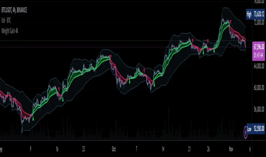
RSI Bollinger Bands [DCAUT]█ RSI Bollinger Bands
📊 ORIGINALITY & INNOVATION
The RSI Bollinger Bands indicator represents a meaningful advancement in momentum analysis by combining two proven technical tools: the Relative Strength Index (RSI) and Bollinger Bands. This combination addresses a significant limitation in traditional RSI analysis - the use of fixed overbought/oversold thresholds (typically 70/30) that fail to adapt to changing market volatility conditions.
Core Innovation:
Rather than relying on static threshold levels, this indicator applies Bollinger Bands statistical analysis directly to RSI values, creating dynamic zones that automatically adjust based on recent momentum volatility. This approach helps reduce false signals during low volatility periods while remaining sensitive to genuine extremes during high volatility conditions.
Key Enhancements Over Traditional RSI:
Dynamic Thresholds: Overbought/oversold zones adapt to market conditions automatically, eliminating the need for manual threshold adjustments across different instruments and timeframes
Volatility Context: Band width provides immediate visual feedback about momentum volatility, helping traders distinguish between stable trends and erratic movements
Reduced False Signals: During ranging markets, narrower bands filter out minor RSI fluctuations that would trigger traditional fixed-threshold signals
Breakout Preparation: Band squeeze patterns (similar to price-based BB) signal potential momentum regime changes before they occur
Self-Referencing Analysis: By measuring RSI against its own statistical behavior rather than arbitrary levels, the indicator provides more relevant context
📐 MATHEMATICAL FOUNDATION
Two-Stage Calculation Process:
Stage 1: RSI Calculation
RSI = 100 - (100 / (1 + RS))
where RS = Average Gain / Average Loss over specified period
The RSI normalizes price momentum into a bounded 0-100 scale, making it ideal for statistical band analysis.
Stage 2: Bollinger Bands on RSI
Basis = MA(RSI, BB Length)
Upper Band = Basis + (StdDev(RSI, BB Length) × Multiplier)
Lower Band = Basis - (StdDev(RSI, BB Length) × Multiplier)
Band Width = Upper Band - Lower Band
The Bollinger Bands measure RSI's standard deviation from its own moving average, creating statistically-derived dynamic zones.
Statistical Interpretation:
Under normal distribution assumptions with default 2.0 multiplier, approximately 95% of RSI values should fall within the bands
Band touches represent statistically significant momentum extremes relative to recent behavior
Band width expansion indicates increasing momentum volatility (strengthening trend or increasing uncertainty)
Band width contraction signals momentum consolidation and potential regime change preparation
📊 COMPREHENSIVE SIGNAL ANALYSIS
Visual Color Signals:
This indicator features dynamic color fills that highlight extreme momentum conditions:
Green Fill (Above Upper Band):
Appears when RSI breaks above the upper band, indicating exceptionally strong bullish momentum
Represents dynamic overbought zone - not necessarily a reversal signal but a warning of extreme conditions
In strong uptrends, green fills can persist as RSI "rides the band" - this indicates sustained momentum strength
Exit of green zone (RSI falling back below upper band) often signals initial momentum weakening
Red Fill (Below Lower Band):
Appears when RSI breaks below the lower band, indicating exceptionally weak bearish momentum
Represents dynamic oversold zone - potential reversal or continuation signal depending on trend context
In strong downtrends, red fills can persist as RSI "rides the band" - this indicates sustained selling pressure
Exit of red zone (RSI rising back above lower band) often signals initial momentum recovery
Position-Based Signals:
Upper Band Interactions:
RSI Touching Upper Band: Dynamic overbought condition - momentum is extremely strong relative to recent volatility, potential exhaustion or continuation depending on trend context
RSI Riding Upper Band: Sustained strong momentum, often seen in powerful trends, not necessarily an immediate reversal signal but warrants monitoring for exhaustion
RSI Crossing Below Upper Band: Initial momentum weakening signal, particularly significant if accompanied by price divergence
Lower Band Interactions:
RSI Touching Lower Band: Dynamic oversold condition - momentum is extremely weak relative to recent volatility, potential reversal or continuation of downtrend
RSI Riding Lower Band: Sustained weak momentum, common in strong downtrends, monitor for potential exhaustion
RSI Crossing Above Lower Band: Initial momentum strengthening signal, early indication of potential reversal or consolidation
Basis Line Signals:
RSI Above Basis: Bullish momentum regime - upward pressure dominant
RSI Below Basis: Bearish momentum regime - downward pressure dominant
Basis Crossovers: Momentum regime shifts, more significant when accompanied by band width changes
RSI Oscillating Around Basis: Balanced momentum, often indicates ranging market conditions
Volatility-Based Signals:
Band Width Patterns:
Narrow Bands (Squeeze): Momentum volatility compression, often precedes significant directional moves, similar to price coiling patterns
Expanding Bands: Increasing momentum volatility, indicates trend acceleration or growing uncertainty
Narrowest Band in 100 Bars: Extreme compression alert, high probability of upcoming volatility expansion
Advanced Pattern Recognition:
Divergence Analysis:
Bullish Divergence: Price makes lower lows while RSI touches or stays above previous lower band touch, suggests downward momentum weakening
Bearish Divergence: Price makes higher highs while RSI touches or stays below previous upper band touch, suggests upward momentum weakening
Hidden Bullish: Price makes higher lows while RSI makes lower lows at the lower band, indicates strong underlying bullish momentum
Hidden Bearish: Price makes lower highs while RSI makes higher highs at the upper band, indicates strong underlying bearish momentum
Band Walk Patterns:
Upper Band Walk: RSI consistently touching or staying near upper band indicates exceptionally strong trend, wait for clear break below basis before considering reversal
Lower Band Walk: RSI consistently at lower band signals very weak momentum, requires break above basis for reversal confirmation
🎯 STRATEGIC APPLICATIONS
Strategy 1: Mean Reversion Trading
Setup Conditions:
Market Type: Ranging or choppy markets with no clear directional trend
Timeframe: Works best on lower timeframes (5m-1H) or during consolidation phases
Band Characteristic: Normal to narrow band width
Entry Rules:
Long Entry: RSI touches or crosses below lower band, wait for RSI to start rising back toward basis before entry
Short Entry: RSI touches or crosses above upper band, wait for RSI to start falling back toward basis before entry
Confirmation: Use price action confirmation (candlestick reversal patterns) at band touches
Exit Rules:
Target: RSI returns to basis line or opposite band
Stop Loss: Fixed percentage or below recent swing low/high
Time Stop: Exit if position not profitable within expected timeframe
Strategy 2: Trend Continuation Trading
Setup Conditions:
Market Type: Clear trending market with higher highs/lower lows
Timeframe: Medium to higher timeframes (1H-Daily)
Band Characteristic: Expanding or wide bands indicating strong momentum
Entry Rules:
Long Entry in Uptrend: Wait for RSI to pull back to basis line or slightly below, enter when RSI starts rising again
Short Entry in Downtrend: Wait for RSI to rally to basis line or slightly above, enter when RSI starts falling again
Avoid Counter-Trend: Do not fade RSI at bands during strong trends (band walk patterns)
Exit Rules:
Trailing Stop: Move stop to break-even when RSI reaches opposite band
Trend Break: Exit when RSI crosses basis against trend direction with conviction
Band Squeeze: Reduce position size when bands start narrowing significantly
Strategy 3: Breakout Preparation
Setup Conditions:
Market Type: Consolidating market after significant move or at key technical levels
Timeframe: Any timeframe, but longer timeframes provide more reliable breakouts
Band Characteristic: Narrowest band width in recent 100 bars (squeeze alert)
Preparation Phase:
Identify band squeeze condition (bands at multi-period narrowest point)
Monitor price action for consolidation patterns (triangles, rectangles, flags)
Prepare bracket orders for both directions
Wait for band expansion to begin
Entry Execution:
Breakout Confirmation: Enter in direction of RSI band breakout (RSI breaks above upper band or below lower band)
Price Confirmation: Ensure price also breaks corresponding technical level
Volume Confirmation: Look for volume expansion supporting the breakout
Risk Management:
Stop Loss: Place beyond consolidation pattern opposite extreme
Position Sizing: Use smaller size due to false breakout risk
Quick Exit: Exit immediately if RSI returns inside bands within 1-3 bars
Strategy 4: Multi-Timeframe Analysis
Timeframe Selection:
Higher Timeframe: Daily or 4H for trend context
Trading Timeframe: 1H or 15m for entry signals
Confirmation Timeframe: 5m or 1m for precise entry timing
Analysis Process:
Trend Identification: Check higher timeframe RSI position relative to bands, trade only in direction of higher timeframe momentum
Setup Formation: Wait for trading timeframe RSI to show pullback to basis in trending direction
Entry Timing: Use confirmation timeframe RSI band touch or crossover for precise entry
Alignment Confirmation: All timeframes should show RSI moving in same direction for highest probability setups
📋 DETAILED PARAMETER CONFIGURATION
RSI Source:
Close (Default): Standard price point, balances responsiveness and reliability
HL2: Reduces noise from intrabar volatility, provides smoother RSI values
HLC3 or OHLC4: Further smoothing for very choppy markets, slower to respond but more stable
Volume-Weighted: Consider using VWAP or volume-weighted prices for additional liquidity context
RSI Length Parameter:
Shorter Periods (5-10): More responsive but generates more signals, suitable for scalping or very active trading, higher noise level
Standard (14): Default and most widely used setting, proven balance between responsiveness and reliability, recommended starting point
Longer Periods (21-30): Smoother momentum measurement, fewer but potentially more reliable signals, better for swing trading or position trading
Optimization Note: Test across different market regimes, optimal length often varies by instrument volatility characteristics
RSI MA Type Parameter:
RMA (Default): Wilder's original smoothing method, provides traditional RSI behavior with balanced lag, most widely recognized and tested, recommended for standard technical analysis
EMA: Exponential smoothing gives more weight to recent values, faster response to momentum changes, suitable for active trading and trending markets, reduces lag compared to RMA
SMA: Simple average treats all periods equally, smoothest output with highest lag, best for filtering noise in choppy markets, useful for long-term position analysis
WMA: Weighted average emphasizes recent data less aggressively than EMA, middle ground between SMA and EMA characteristics, balanced responsiveness for swing trading
Advanced Options: Full access to 25+ moving average types including HMA (reduced lag), DEMA/TEMA (enhanced responsiveness), KAMA/FRAMA (adaptive behavior), T3 (smoothness), Kalman Filter (optimal estimation)
Selection Guide: RMA for traditional analysis and backtesting consistency, EMA for faster signals in trending markets, SMA for stability in ranging markets, adaptive types (KAMA/FRAMA) for varying volatility regimes
BB Length Parameter:
Short Length (10-15): Tighter bands that react quickly to RSI changes, more frequent band touches, suitable for active trading styles
Standard (20): Balanced approach providing meaningful statistical context without excessive lag
Long Length (30-50): Smoother bands that filter minor RSI fluctuations, captures only significant momentum extremes, fewer but higher quality signals
Relationship to RSI Length: Consider BB Length greater than RSI Length for cleaner signals
BB MA Type Parameter:
SMA (Default): Standard Bollinger Bands calculation using simple moving average for basis line, treats all periods equally, widely recognized and tested approach
EMA: Exponential smoothing for basis line gives more weight to recent RSI values, creates more responsive bands that adapt faster to momentum changes, suitable for trending markets
RMA: Wilder's smoothing provides consistent behavior aligned with traditional RSI when using RMA for both RSI and BB calculations
WMA: Weighted average for basis line balances recent emphasis with historical context, middle ground between SMA and EMA responsiveness
Advanced Options: Full access to 25+ moving average types for basis calculation, including HMA (reduced lag), DEMA/TEMA (enhanced responsiveness), KAMA/FRAMA (adaptive to volatility changes)
Selection Guide: SMA for standard Bollinger Bands behavior and backtesting consistency, EMA for faster band adaptation in dynamic markets, matching RSI MA type creates unified smoothing behavior
BB Multiplier Parameter:
Conservative (1.5-1.8): Tighter bands resulting in more frequent touches, useful in low volatility environments, higher signal frequency but potentially more false signals
Standard (2.0): Default setting representing approximately 95% confidence interval under normal distribution, widely accepted statistical threshold
Aggressive (2.5-3.0): Wider bands capturing only extreme momentum conditions, fewer but potentially more significant signals, reduces false signals in high volatility
Adaptive Approach: Consider adjusting multiplier based on instrument characteristics, lower multiplier for stable instruments, higher for volatile instruments
Parameter Optimization Workflow:
Start with default parameters (RSI:14, BB:20, Mult:2.0)
Test across representative sample period including different market regimes
Adjust RSI length based on desired responsiveness vs stability tradeoff
Tune BB length to match your typical holding period
Modify multiplier to achieve desired signal frequency
Validate on out-of-sample data to avoid overfitting
Document optimal parameters for different instruments and timeframes
Reference Levels Display:
Enabled (Default): Shows traditional 30/50/70 levels for comparison with dynamic bands, helps visualize the adaptive advantage
Disabled: Cleaner chart focusing purely on dynamic zones, reduces visual clutter for experienced users
Educational Value: Keeping reference levels visible helps understand how dynamic bands differ from fixed thresholds across varying market conditions
📈 PERFORMANCE ANALYSIS & COMPETITIVE ADVANTAGES
Comparison with Traditional RSI:
Fixed Threshold RSI Limitations:
In ranging low-volatility markets: RSI rarely reaches 70/30, missing tradable extremes
In trending high-volatility markets: RSI frequently breaks through 70/30, generating excessive false reversal signals
Across different instruments: Same thresholds applied to volatile crypto and stable forex pairs produce inconsistent results
Threshold Adjustment Problem: Manually changing thresholds for different conditions is subjective and lagging
RSI Bollinger Bands Advantages:
Automatic Adaptation: Bands adjust to current volatility regime without manual intervention
Consistent Logic: Same statistical approach works across different instruments and timeframes
Reduced False Signals: Band width filtering helps distinguish meaningful extremes from noise
Additional Information: Band width provides volatility context missing in standard RSI
Objective Extremes: Statistical basis (standard deviations) provides objective extreme definition
Comparison with Price-Based Bollinger Bands:
Price BB Characteristics:
Measures absolute price volatility
Affected by large price gaps and outliers
Band position relative to price not normalized
Difficult to compare across different price scales
RSI BB Advantages:
Normalized Scale: RSI's 0-100 bounds make band interpretation consistent across all instruments
Momentum Focus: Directly measures momentum extremes rather than price extremes
Reduced Gap Impact: RSI calculation smooths price gaps impact on band calculations
Comparable Analysis: Same RSI BB appearance across stocks, forex, crypto enables consistent strategy application
Performance Characteristics:
Signal Quality:
Higher Signal-to-Noise Ratio: Dynamic bands help filter RSI oscillations that don't represent meaningful extremes
Context-Aware Alerts: Band width provides volatility context helping traders adjust position sizing and stop placement
Reduced Whipsaws: During consolidations, narrower bands prevent premature signals from minor RSI movements
Responsiveness:
Adaptive Lag: Band calculation introduces some lag, but this lag is adaptive to current conditions rather than fixed
Faster Than Manual Adjustment: Automatic band adjustment is faster than trader's ability to manually modify thresholds
Balanced Approach: Combines RSI's inherent momentum lag with BB's statistical smoothing for stable yet responsive signals
Versatility:
Multi-Strategy Application: Supports both mean reversion (ranging markets) and trend continuation (trending markets) approaches
Universal Instrument Coverage: Works effectively across equities, forex, commodities, cryptocurrencies without parameter changes
Timeframe Agnostic: Same interpretation applies from 1-minute charts to monthly charts
Limitations and Considerations:
Known Limitations:
Dual Lag Effect: Combines RSI's momentum lag with BB's statistical lag, making it less suitable for very short-term scalping
Requires Volatility History: Needs sufficient bars for BB calculation, less effective immediately after major regime changes
Statistical Assumptions: Assumes RSI values are somewhat normally distributed, extreme trending conditions may violate this
Not a Standalone System: Like all indicators, should be combined with price action analysis and risk management
Optimal Use Cases:
Best for swing trading and position trading timeframes
Most effective in markets with alternating volatility regimes
Ideal for traders who use multiple instruments and timeframes
Suitable for systematic trading approaches requiring consistent logic
Suboptimal Conditions:
Very low timeframes (< 5 minutes) where lag becomes problematic
Instruments with extreme volatility spikes (gap-prone markets)
Markets in strong persistent trends where mean reversion rarely occurs
Periods immediately following major structural changes (new trading regime)
USAGE NOTES
This indicator is designed for technical analysis and educational purposes to help traders understand the interaction between momentum measurement and statistical volatility bands. The RSI Bollinger Bands has limitations and should not be used as the sole basis for trading decisions.
Important Considerations:
No Predictive Guarantee: Past band touches and patterns do not guarantee future price behavior
Market Regime Dependency: Indicator performance varies significantly between trending and ranging market conditions
Complementary Analysis Required: Should be used alongside price action, support/resistance levels, and fundamental analysis
Risk Management Essential: Always use proper position sizing, stop losses, and risk controls regardless of signal quality
Parameter Sensitivity: Different instruments and timeframes may require parameter optimization for optimal results
Continuous Monitoring: Band characteristics change with market conditions, requiring ongoing assessment
Recommended Supporting Analysis:
Price structure analysis (support/resistance, trend lines)
Volume confirmation for breakout signals
Multiple timeframe alignment
Market context awareness (news events, session times)
Correlation analysis with related instruments
The indicator aims to provide adaptive momentum analysis that adjusts to changing market volatility, but traders must apply sound judgment, proper risk management, and comprehensive market analysis in their decision-making process.

Stochastic Enhanced [DCAUT]█ Stochastic Enhanced
📊 ORIGINALITY & INNOVATION
The Stochastic Enhanced indicator builds upon George Lane's classic momentum oscillator (developed in the late 1950s) by providing comprehensive smoothing algorithm flexibility. While traditional implementations limit users to Simple Moving Average (SMA) smoothing, this enhanced version offers 21 advanced smoothing algorithms, allowing traders to optimize the indicator's characteristics for different market conditions and trading styles.
Key Improvements:
Extended from single SMA smoothing to 21 professional-grade algorithms including adaptive filters (KAMA, FRAMA), zero-lag methods (ZLEMA, T3), and advanced digital filters (Kalman, Laguerre)
Maintains backward compatibility with traditional Stochastic calculations through SMA default setting
Unified smoothing algorithm applies to both %K and %D lines for consistent signal processing characteristics
Enhanced visual feedback with clear color distinction and background fill highlighting for intuitive signal recognition
Comprehensive alert system covering crossovers and zone entries for systematic trade management
Differentiation from Traditional Stochastic:
Traditional Stochastic indicators use fixed SMA smoothing, which introduces consistent lag regardless of market volatility. This enhanced version addresses the limitation by offering adaptive algorithms that adjust to market conditions (KAMA, FRAMA), reduce lag without sacrificing smoothness (ZLEMA, T3, HMA), or provide superior noise filtering (Kalman Filter, Laguerre filters). The flexibility helps traders balance responsiveness and stability according to their specific needs.
📐 MATHEMATICAL FOUNDATION
Core Stochastic Calculation:
The Stochastic Oscillator measures the position of the current close relative to the high-low range over a specified period:
Step 1: Raw %K Calculation
%K_raw = 100 × (Close - Lowest Low) / (Highest High - Lowest Low)
Where:
Close = Current closing price
Lowest Low = Lowest low over the %K Length period
Highest High = Highest high over the %K Length period
Result ranges from 0 (close at period low) to 100 (close at period high)
Step 2: Smoothed %K Calculation
%K = MA(%K_raw, K Smoothing Period, MA Type)
Where:
MA = Selected moving average algorithm (SMA, EMA, etc.)
K Smoothing = 1 for Fast Stochastic, 3+ for Slow Stochastic
Traditional Fast Stochastic uses %K_raw directly without smoothing
Step 3: Signal Line %D Calculation
%D = MA(%K, D Smoothing Period, MA Type)
Where:
%D acts as a signal line and moving average of %K
D Smoothing typically set to 3 periods in traditional implementations
Both %K and %D use the same MA algorithm for consistent behavior
Available Smoothing Algorithms (21 Options):
Standard Moving Averages:
SMA (Simple): Equal-weighted average, traditional default, consistent lag characteristics
EMA (Exponential): Recent price emphasis, faster response to changes, exponential decay weighting
RMA (Rolling/Wilder's): Smoothed average used in RSI, less reactive than EMA
WMA (Weighted): Linear weighting favoring recent data, moderate responsiveness
VWMA (Volume-Weighted): Incorporates volume data, reflects market participation intensity
Advanced Moving Averages:
HMA (Hull): Reduced lag with smoothness, uses weighted moving averages and square root period
ALMA (Arnaud Legoux): Gaussian distribution weighting, minimal lag with good noise reduction
LSMA (Least Squares): Linear regression based, fits trend line to data points
DEMA (Double Exponential): Reduced lag compared to EMA, uses double smoothing technique
TEMA (Triple Exponential): Further lag reduction, triple smoothing with lag compensation
ZLEMA (Zero-Lag Exponential): Lag elimination attempt using error correction, very responsive
TMA (Triangular): Double-smoothed SMA, very smooth but slower response
Adaptive & Intelligent Filters:
T3 (Tilson T3): Six-pass exponential smoothing with volume factor adjustment, excellent smoothness
FRAMA (Fractal Adaptive): Adapts to market fractal dimension, faster in trends, slower in ranges
KAMA (Kaufman Adaptive): Efficiency ratio based adaptation, responds to volatility changes
McGinley Dynamic: Self-adjusting mechanism following price more accurately, reduced whipsaws
Kalman Filter: Optimal estimation algorithm from aerospace engineering, dynamic noise filtering
Advanced Digital Filters:
Ultimate Smoother: Advanced digital filter design, superior noise rejection with minimal lag
Laguerre Filter: Time-domain filter with N-order implementation, adjustable lag characteristics
Laguerre Binomial Filter: 6-pole Laguerre filter, extremely smooth output for long-term analysis
Super Smoother: Butterworth filter implementation, removes high-frequency noise effectively
📊 COMPREHENSIVE SIGNAL ANALYSIS
Absolute Level Interpretation (%K Line):
%K Above 80: Overbought condition, price near period high, potential reversal or pullback zone, caution for new long entries
%K in 70-80 Range: Strong upward momentum, bullish trend confirmation, uptrend likely continuing
%K in 50-70 Range: Moderate bullish momentum, neutral to positive outlook, consolidation or mild uptrend
%K in 30-50 Range: Moderate bearish momentum, neutral to negative outlook, consolidation or mild downtrend
%K in 20-30 Range: Strong downward momentum, bearish trend confirmation, downtrend likely continuing
%K Below 20: Oversold condition, price near period low, potential bounce or reversal zone, caution for new short entries
Crossover Signal Analysis:
%K Crosses Above %D (Bullish Cross): Momentum shifting bullish, faster line overtakes slower signal, consider long entry especially in oversold zone, strongest when occurring below 20 level
%K Crosses Below %D (Bearish Cross): Momentum shifting bearish, faster line falls below slower signal, consider short entry especially in overbought zone, strongest when occurring above 80 level
Crossover in Midrange (40-60): Less reliable signals, often in choppy sideways markets, require additional confirmation from trend or volume analysis
Multiple Failed Crosses: Indicates ranging market or choppy conditions, reduce position sizes or avoid trading until clear directional move
Advanced Divergence Patterns (%K Line vs Price):
Bullish Divergence: Price makes lower low while %K makes higher low, indicates weakening bearish momentum, potential trend reversal upward, more reliable when %K in oversold zone
Bearish Divergence: Price makes higher high while %K makes lower high, indicates weakening bullish momentum, potential trend reversal downward, more reliable when %K in overbought zone
Hidden Bullish Divergence: Price makes higher low while %K makes lower low, indicates trend continuation in uptrend, bullish trend strength confirmation
Hidden Bearish Divergence: Price makes lower high while %K makes higher high, indicates trend continuation in downtrend, bearish trend strength confirmation
Momentum Strength Analysis (%K Line Slope):
Steep %K Slope: Rapid momentum change, strong directional conviction, potential for extended moves but also increased reversal risk
Gradual %K Slope: Steady momentum development, sustainable trends more likely, lower probability of sharp reversals
Flat or Horizontal %K: Momentum stalling, potential reversal or consolidation ahead, wait for directional break before committing
%K Oscillation Within Range: Indicates ranging market, sideways price action, better suited for range-trading strategies than trend following
🎯 STRATEGIC APPLICATIONS
Mean Reversion Strategy (Range-Bound Markets):
Identify ranging market conditions using price action or Bollinger Bands
Wait for Stochastic to reach extreme zones (above 80 for overbought, below 20 for oversold)
Enter counter-trend position when %K crosses %D in extreme zone (sell on bearish cross above 80, buy on bullish cross below 20)
Set profit targets near opposite extreme or midline (50 level)
Use tight stop-loss above recent swing high/low to protect against breakout scenarios
Exit when Stochastic reaches opposite extreme or %K crosses %D in opposite direction
Trend Following with Momentum Confirmation:
Identify primary trend direction using higher timeframe analysis or moving averages
Wait for Stochastic pullback to oversold zone (<20) in uptrend or overbought zone (>80) in downtrend
Enter in trend direction when %K crosses %D confirming momentum shift (bullish cross in uptrend, bearish cross in downtrend)
Use wider stops to accommodate normal trend volatility
Add to position on subsequent pullbacks showing similar Stochastic pattern
Exit when Stochastic shows opposite extreme with failed cross or bearish/bullish divergence
Divergence-Based Reversal Strategy:
Scan for divergence between price and Stochastic at swing highs/lows
Confirm divergence with at least two price pivots showing divergent Stochastic readings
Wait for %K to cross %D in direction of anticipated reversal as entry trigger
Enter position in divergence direction with stop beyond recent swing extreme
Target profit at key support/resistance levels or Fibonacci retracements
Scale out as Stochastic reaches opposite extreme zone
Multi-Timeframe Momentum Alignment:
Analyze Stochastic on higher timeframe (4H or Daily) for primary trend bias
Switch to lower timeframe (1H or 15M) for precise entry timing
Only take trades where lower timeframe Stochastic signal aligns with higher timeframe momentum direction
Higher timeframe Stochastic in bullish zone (>50) = only take long entries on lower timeframe
Higher timeframe Stochastic in bearish zone (<50) = only take short entries on lower timeframe
Exit when lower timeframe shows counter-signal or higher timeframe momentum reverses
Zone Transition Strategy:
Monitor Stochastic for transitions between zones (oversold to neutral, neutral to overbought, etc.)
Enter long when Stochastic crosses above 20 (exiting oversold), signaling momentum shift from bearish to neutral/bullish
Enter short when Stochastic crosses below 80 (exiting overbought), signaling momentum shift from bullish to neutral/bearish
Use zone midpoint (50) as dynamic support/resistance for position management
Trail stops as Stochastic advances through favorable zones
Exit when Stochastic fails to maintain momentum and reverses back into prior zone
📋 DETAILED PARAMETER CONFIGURATION
%K Length (Default: 14):
Lower Values (5-9): Highly sensitive to price changes, generates more frequent signals, increased false signals in choppy markets, suitable for very short-term trading and scalping
Standard Values (10-14): Balanced sensitivity and reliability, traditional default (14) widely used,适合 swing trading and intraday strategies
Higher Values (15-21): Reduced sensitivity, smoother oscillations, fewer but potentially more reliable signals, better for position trading and lower timeframe noise reduction
Very High Values (21+): Slow response, long-term momentum measurement, fewer trading signals, suitable for weekly or monthly analysis
%K Smoothing (Default: 3):
Value 1: Fast Stochastic, uses raw %K calculation without additional smoothing, most responsive to price changes, generates earliest signals with higher noise
Value 3: Slow Stochastic (default), traditional smoothing level, reduces false signals while maintaining good responsiveness, widely accepted standard
Values 5-7: Very slow response, extremely smooth oscillations, significantly reduced whipsaws but delayed entry/exit timing
Recommendation: Default value 3 suits most trading scenarios, active short-term traders may use 1, conservative long-term positions use 5+
%D Smoothing (Default: 3):
Lower Values (1-2): Signal line closely follows %K, frequent crossover signals, useful for active trading but requires strict filtering
Standard Value (3): Traditional setting providing balanced signal line behavior, optimal for most trading applications
Higher Values (4-7): Smoother signal line, fewer crossover signals, reduced whipsaws but slower confirmation, better for trend trading
Very High Values (8+): Signal line becomes slow-moving reference, crossovers rare and highly significant, suitable for long-term position changes only
Smoothing Type Algorithm Selection:
For Trending Markets:
ZLEMA, DEMA, TEMA: Reduced lag for faster trend entry, quick response to momentum shifts, suitable for strong directional moves
HMA, ALMA: Good balance of smoothness and responsiveness, effective for clean trend following without excessive noise
EMA: Classic choice for trending markets, faster than SMA while maintaining reasonable stability
For Ranging/Choppy Markets:
Kalman Filter, Super Smoother: Superior noise filtering, reduces false signals in sideways action, helps identify genuine reversal points
Laguerre Filters: Smooth oscillations with adjustable lag, excellent for mean reversion strategies in ranges
T3, TMA: Very smooth output, filters out market noise effectively, clearer extreme zone identification
For Adaptive Market Conditions:
KAMA: Automatically adjusts to market efficiency, fast in trends and slow in congestion, reduces whipsaws during transitions
FRAMA: Adapts to fractal market structure, responsive during directional moves, conservative during uncertainty
McGinley Dynamic: Self-adjusting smoothing, follows price naturally, minimizes lag in trending markets while filtering noise in ranges
For Conservative Long-Term Analysis:
SMA: Traditional choice, predictable behavior, widely understood characteristics
RMA (Wilder's): Smooth oscillations, reduced sensitivity to outliers, consistent behavior across market conditions
Laguerre Binomial Filter: Extremely smooth output, ideal for weekly/monthly timeframe analysis, eliminates short-term noise completely
Source Selection:
Close (Default): Standard choice using closing prices, most common and widely tested
HLC3 or OHLC4: Incorporates more price information, reduces impact of sudden spikes or gaps, smoother oscillator behavior
HL2: Midpoint of high-low range, emphasizes intrabar volatility, useful for markets with wide intraday ranges
Custom Source: Can use other indicators as input (e.g., Heikin Ashi close, smoothed price), creates derivative momentum indicators
📈 PERFORMANCE ANALYSIS & COMPETITIVE ADVANTAGES
Responsiveness Characteristics:
Traditional SMA-Based Stochastic:
Fixed lag regardless of market conditions, consistent delay of approximately (K Smoothing + D Smoothing) / 2 periods
Equal treatment of trending and ranging markets, no adaptation to volatility changes
Predictable behavior but suboptimal in varying market regimes
Enhanced Version with Adaptive Algorithms:
KAMA and FRAMA reduce lag by up to 40-60% in strong trends compared to SMA while maintaining similar smoothness in ranges
ZLEMA and T3 provide near-zero lag characteristics for early entry signals with acceptable noise levels
Kalman Filter and Super Smoother offer superior noise rejection, reducing false signals in choppy conditions by estimations of 30-50% compared to SMA
Performance improvements vary by algorithm selection and market conditions
Signal Quality Improvements:
Adaptive algorithms help reduce whipsaw trades in ranging markets by adjusting sensitivity dynamically
Advanced filters (Kalman, Laguerre, Super Smoother) provide clearer extreme zone readings for mean reversion strategies
Zero-lag methods (ZLEMA, DEMA, TEMA) generate earlier crossover signals in trending markets for improved entry timing
Smoother algorithms (T3, Laguerre Binomial) reduce false extreme zone touches for more reliable overbought/oversold signals
Comparison with Standard Implementations:
Versus Basic Stochastic: Enhanced version offers 21 smoothing options versus single SMA, allowing optimization for specific market characteristics and trading styles
Versus RSI: Stochastic provides range-bound measurement (0-100) with clear extreme zones, RSI measures momentum speed, Stochastic offers clearer visual overbought/oversold identification
Versus MACD: Stochastic bounded oscillator suitable for mean reversion, MACD unbounded indicator better for trend strength, Stochastic excels in range-bound and oscillating markets
Versus CCI: Stochastic has fixed bounds (0-100) for consistent interpretation, CCI unbounded with variable extremes, Stochastic provides more standardized extreme readings across different instruments
Flexibility Advantages:
Single indicator adaptable to multiple strategies through algorithm selection rather than requiring different indicator variants
Ability to optimize smoothing characteristics for specific instruments (e.g., smoother for crypto volatility, faster for forex trends)
Multi-timeframe analysis with consistent algorithm across timeframes for coherent momentum picture
Backtesting capability with algorithm as optimization parameter for strategy development
Limitations and Considerations:
Increased complexity from multiple algorithm choices may lead to over-optimization if parameters are curve-fitted to historical data
Adaptive algorithms (KAMA, FRAMA) have adjustment periods during market regime changes where signals may be less reliable
Zero-lag algorithms sacrifice some smoothness for responsiveness, potentially increasing noise sensitivity in very choppy conditions
Performance characteristics vary significantly across algorithms, requiring understanding and testing before live implementation
Like all oscillators, Stochastic can remain in extreme zones for extended periods during strong trends, generating premature reversal signals
USAGE NOTES
This indicator is designed for technical analysis and educational purposes to provide traders with enhanced flexibility in momentum analysis. The Stochastic Oscillator has limitations and should not be used as the sole basis for trading decisions.
Important Considerations:
Algorithm performance varies with market conditions - no single smoothing method is optimal for all scenarios
Extreme zone signals (overbought/oversold) indicate potential reversal areas but not guaranteed turning points, especially in strong trends
Crossover signals may generate false entries during sideways choppy markets regardless of smoothing algorithm
Divergence patterns require confirmation from price action or additional indicators before trading
Past indicator characteristics and backtested results do not guarantee future performance
Always combine Stochastic analysis with proper risk management, position sizing, and multi-indicator confirmation
Test selected algorithm on historical data of specific instrument and timeframe before live trading
Market regime changes may require algorithm adjustment for optimal performance
The enhanced smoothing options are intended to provide tools for optimizing the indicator's behavior to match individual trading styles and market characteristics, not to create a perfect predictive tool. Responsible usage includes understanding the mathematical properties of selected algorithms and their appropriate application contexts.

T3 [DCAUT]█ T3
📊 INDICATOR OVERVIEW
The T3 Moving Average is a smoothing indicator developed by Tim Tillson and published in Technical Analysis of Stocks & Commodities magazine (January 1998). The algorithm applies Generalized DEMA (Double Exponential Moving Average) recursively three times, creating a six-pole filtering effect that aims to balance noise reduction with responsiveness while minimizing lag relative to price changes.
📐 MATHEMATICAL FOUNDATION
Generalized DEMA (GD) Function:
The core building block is the Generalized DEMA function, which combines two exponential moving averages with weights controlled by the volume factor:
GD(input, v) = EMA(input) × (1 + v) - EMA(EMA(input)) × v
Where v is the volume factor parameter (default 0.7). This weighted combination reduces lag while maintaining smoothness by extrapolating beyond the first EMA using the double-smoothed EMA as a reference.
T3 Calculation Process:
T3 applies the GD function three times recursively:
T3 = GD(GD(GD(Price, v), v), v)
This triple nesting creates a six-pole smoothing effect (each GD applies two EMA operations, resulting in 2 × 3 = 6 total EMA calculations). The cascading refinement progressively filters noise while preserving trend information.
Step-by-Step Breakdown:
First GD application: GD1 = EMA(Price) × (1 + v) - EMA(EMA(Price)) × v - Creates initial smoothed series with lag reduction
Second GD application: GD2 = EMA(GD1) × (1 + v) - EMA(EMA(GD1)) × v - Further refines the smoothing while maintaining responsiveness
Third GD application: T3 = EMA(GD2) × (1 + v) - EMA(EMA(GD2)) × v - Final refinement produces the T3 output
Volume Factor Impact:
The volume factor (v) is the key parameter controlling the balance between smoothness and responsiveness. Tim Tillson recommended v = 0.7 as the optimal default value.
Lower volume factors (v closer to 0.0): Increase the extrapolation effect, making T3 more responsive to price changes but potentially more sensitive to noise.
Higher volume factors (v closer to 1.0): Reduce the extrapolation effect, producing smoother output with less sensitivity to short-term fluctuations but slightly more lag.
The recursive application of the volume factor through three GD stages creates a nonlinear filtering effect that achieves superior lag reduction compared to traditional moving averages of equivalent smoothness.
📊 SIGNAL INTERPRETATION
Trend Direction Signals:
Green Line (T3 Rising): Smoothed trend line is rising, may indicate uptrend, consider bullish opportunities when confirmed by other factors
Red Line (T3 Falling): Smoothed trend line is falling, may indicate downtrend, consider bearish opportunities when confirmed by other factors
Gray Line (T3 Flat): Smoothed trend line is flat, indicates unclear trend or consolidation phase
Price Crossover Signals:
Price Crosses Above T3: Price breaks above smoothed trend line, may be bullish signal, requires confirmation from other indicators
Price Crosses Below T3: Price breaks below smoothed trend line, may be bearish signal, requires confirmation from other indicators
Price Position Relative to T3: Price sustained above T3 may indicate uptrend, sustained below may indicate downtrend
Supporting Analysis Signals:
T3 Slope Angle: Steeper slopes indicate stronger trend momentum, flatter slopes suggest weakening trends
Price Deviation: Significant price separation from T3 may indicate overextension, watch for pullback or reversal
Dynamic Support/Resistance: T3 line can serve as dynamic support (in uptrends) or resistance (in downtrends) reference
🎯 STRATEGIC APPLICATIONS
Common Usage Patterns:
The T3 Moving Average can be incorporated into trading analysis in various ways. These represent common approaches used by market participants, though effectiveness varies by market conditions and requires individual testing:
Trend Filtering:
T3 can be used as a trend filter by observing the relationship between price and the T3 line. The color-coded slope (green for rising, red for falling, gray for sideways) provides visual feedback about the current trend direction of the smoothed series.
Price Crossover Analysis:
Some traders monitor crossovers between price and the T3 line as potential indication points. When price crosses the T3 line, it may suggest a change in the relationship between current price action and the smoothed trend.
Multi-Timeframe Observation:
T3 can be applied to multiple timeframes simultaneously. Observing alignment or divergence between different timeframe T3 indicators may provide context about trend consistency across time scales.
Dynamic Reference Level:
The T3 line can serve as a dynamic reference level for price action analysis. Price distance from T3, price reactions when approaching T3, and the behavior of price relative to the T3 line can all be incorporated into market analysis frameworks.
Application Considerations:
Any trading application should be thoroughly tested on historical data before implementation
T3 performance characteristics vary across different market conditions and asset types
The indicator provides smoothed trend information but does not predict future price movements
Combining T3 with other analytical tools and market context improves analysis quality
Risk management practices remain essential regardless of the analytical approach used
📋 DETAILED PARAMETER CONFIGURATION
Source Selection:
Close Price (Default): Standard choice for end-of-period trend analysis, reduces intrabar noise
HL2 (High+Low)/2: Provides balanced view of price action, considers full bar range
HLC3 or OHLC4: Incorporates more price information, may provide smoother results
Selection Impact: Different sources affect signal timing and smoothness characteristics
Length Configuration:
Shorter periods: More responsive, faster reaction, frequent signals, but higher false signal risk in choppy markets
Longer periods: Smoother output, fewer signals, better for long-term trends, but slower response
Default 14 periods is a common baseline, but optimal length varies by asset, timeframe, and market conditions
Parameter selection should be determined through backtesting rather than general recommendations
Volume Factor Configuration:
Lower values (closer to 0.0): Increase responsiveness but also noise sensitivity
Higher values (closer to 1.0): Increase smoothness but slightly more lag
Default 0.7 (Tim Tillson's recommendation) provides good balance for most applications
Optimal value depends on signal frequency versus reliability preference, test for specific use case
Parameter Optimization Approach:
There are no universal "best" parameter values - optimal settings depend on the specific asset, timeframe, market regime, and trading strategy
Start with default values (Length: 14, Volume Factor: 0.7) and adjust based on observed performance in your target market
Conduct systematic backtesting across different market conditions to evaluate parameter sensitivity
Consider that parameters optimized for historical data may not perform identically in future market conditions
Monitor performance and be prepared to adjust parameters as market characteristics evolve
📈 DESIGN FEATURES & MARKET ADAPTATION
Algorithm Design Features:
Simple Moving Average (SMA): Equal weighting across lookback period
Exponential Moving Average (EMA): Exponentially decreasing weights on historical prices
T3 Moving Average: Recursive Generalized DEMA with adjustable volume factor
Market Condition Adaptation:
Trending markets: Smoothed indicators generally align more closely with sustained directional movement
Ranging markets: All moving averages may generate more crossover signals during non-trending periods
Volatile conditions: Higher smoothing parameters reduce short-term sensitivity but increase lag
Indicator behavior relative to market conditions should be evaluated for specific applications
USAGE NOTES
This indicator is designed for technical analysis and educational purposes. The T3 Moving Average has limitations and should not be used as the sole basis for trading decisions. Like all trend-following indicators, its performance varies with market conditions, and past signal characteristics do not guarantee future results.
Key Points:
T3 is a lagging indicator that responds to price changes rather than predicting future movements
Signals should be confirmed with other technical tools and market context
Parameters should be optimized for specific market and timeframe
Risk management and position sizing are essential
Market regime changes can affect indicator effectiveness
Test strategies thoroughly on historical data before live implementation
Consider broader market context and fundamental factors