CCY Relative Strength [USD]This script provides an indication of the USD relative strength against other major currencies.
The strength is denoted by sma(roc(close, p1), p2). The USD value is always 0.
p1: SMA Period
p2: ROC Period
If you set the SMA Period to 1, it simply functions as the ROC.
Pesquisar nos scripts por "CCI"

CCI MACDWe usually use closing prices for MACD calculations.
However, this indicator is calculated using CCI.
CCI Secret Sauce 1hr strategy by CryptoLloydChanged the CCI_Period to 30 and T3_Period to 1
Giving us a much clear indication of when to go long or short when used with RSI and MACD.
Rules:
LONG - RSI above 50, MACD Bullish cross - Use common sense, price action, horizontal support/resistance, 55 and 150 EMA's
SHORT - Inverse rule set - Use common sense, price action, horizontal support/resistance, 55 and 150 EMA's

CCI trend and extreme indicatorThis employ multi time frame analysis to give a good visual of where is the market is at.
green = general market is trending up from the confluence of 3 different time frame
red = general market is trending down from the confluence of 3 different time frame
Bright green = overbought and trend is likely to reverse
Bright red = oversold and trend is likely to reverse

Scout Regiment - KSI# Scout Regiment - KSI Indicator
## English Documentation
### Overview
Scout Regiment - KSI (Key Stochastic Indicators) is a comprehensive momentum oscillator that combines three powerful technical indicators - RSI, CCI, and Williams %R - into a single, unified display. This multi-indicator approach provides traders with diverse perspectives on market momentum, overbought/oversold conditions, and potential reversal points through advanced divergence detection.
### What is KSI?
KSI stands for "Key Stochastic Indicators" - a composite momentum indicator that:
- Displays multiple oscillators normalized to a 0-100 scale
- Uses standardized bands (20/50/80) for consistent interpretation
- Combines RSI for trend, CCI for cycle, and Williams %R for reversal detection
- Provides enhanced divergence detection specifically for RSI
### Key Features
#### 1. **Triple Oscillator System**
**① RSI (Relative Strength Index)** - Primary Indicator
- **Purpose**: Measures momentum and identifies overbought/oversold conditions
- **Default Length**: 22 periods
- **Display**: Blue line (2px)
- **Key Levels**:
- Above 50: Bullish momentum
- Below 50: Bearish momentum
- Above 80: Overbought
- Below 20: Oversold
- **Special Features**:
- Background color indication (green/red)
- Crossover labels at 50 level
- Full divergence detection (4 types)
**② CCI (Commodity Channel Index)** - Dual Period
- **Purpose**: Identifies cyclical trends and extreme conditions
- **Dual Display**:
- CCI(33): Short-term cycle - Green line (1px)
- CCI(77): Medium-term cycle - Orange line (1px)
- **Default Source**: HLC3 (typical price)
- **Normalized Scale**: Mapped from ±100 to 0-100 for consistency
- **Interpretation**:
- Above 80: Strong upward momentum
- Below 20: Strong downward momentum
- 50 level: Neutral
- Divergence between periods: Trend change warning
**③ Williams %R** - Optional
- **Purpose**: Identifies overbought/oversold extremes
- **Default Length**: 28 periods
- **Display**: Magenta line (2px)
- **Scale**: Inverted and normalized to 0-100
- **Best For**: Short-term reversal signals
- **Default**: Disabled (enable when needed for extra confirmation)
#### 2. **Standardized Band System**
**Three-Level Structure:**
- **Upper Band (80)**: Overbought zone
- Strong momentum area
- Watch for reversal signals
- Divergences here are most reliable
- **Middle Line (50)**: Equilibrium
- Separates bullish/bearish zones
- Crossovers indicate momentum shifts
- Key decision level
- **Lower Band (20)**: Oversold zone
- Weak momentum area
- Look for bounce signals
- Divergences here signal potential reversals
**Band Fill**: Dark background between 20-80 for visual clarity
#### 3. **RSI Visual Enhancements**
**Background Color Indication**
- Green background: RSI above 50 (bullish bias)
- Red background: RSI below 50 (bearish bias)
- Optional display for cleaner charts
- Helps identify overall momentum direction
**Crossover Labels**
- "突破" (Breakout): RSI crosses above 50
- "跌破" (Breakdown): RSI crosses below 50
- Marks momentum shift points
- Can be toggled on/off
#### 4. **Advanced RSI Divergence Detection**
The indicator includes comprehensive divergence detection for RSI only (most reliable oscillator):
**Regular Bullish Divergence (Yellow)**
- **Price**: Lower lows
- **RSI**: Higher lows
- **Signal**: Potential upward reversal
- **Label**: "涨" (Up)
- **Most Common**: Near oversold levels (below 30)
**Regular Bearish Divergence (Blue)**
- **Price**: Higher highs
- **RSI**: Lower highs
- **Signal**: Potential downward reversal
- **Label**: "跌" (Down)
- **Most Common**: Near overbought levels (above 70)
**Hidden Bullish Divergence (Light Yellow)**
- **Price**: Higher lows
- **RSI**: Lower lows
- **Signal**: Uptrend continuation
- **Label**: "隐涨" (Hidden Up)
- **Use**: Add to existing longs
**Hidden Bearish Divergence (Light Blue)**
- **Price**: Lower highs
- **RSI**: Higher highs
- **Signal**: Downtrend continuation
- **Label**: "隐跌" (Hidden Down)
- **Use**: Add to existing shorts
**Divergence Parameters** (Fully Customizable):
- **Right Lookback**: Bars to right of pivot (default: 5)
- **Left Lookback**: Bars to left of pivot (default: 5)
- **Max Range**: Maximum bars between pivots (default: 60)
- **Min Range**: Minimum bars between pivots (default: 5)
### Configuration Settings
#### KSI Display Settings
- **Show RSI**: Toggle RSI indicator
- **Show CCI**: Toggle both CCI lines
- **Show Williams %R**: Toggle Williams %R (optional)
#### RSI Settings
- **RSI Length**: Period for calculation (default: 22)
- **Data Source**: Price source (default: close)
- **Show Background**: Toggle green/red background
- **Show Cross Labels**: Toggle 50-level crossover labels
#### RSI Divergence Settings
- **Right Lookback**: Pivot detection right side
- **Left Lookback**: Pivot detection left side
- **Max Range**: Maximum lookback distance
- **Min Range**: Minimum lookback distance
- **Show Regular Divergence**: Enable regular divergence lines
- **Show Regular Labels**: Enable regular divergence labels
- **Show Hidden Divergence**: Enable hidden divergence lines
- **Show Hidden Labels**: Enable hidden divergence labels
#### CCI Settings
- **CCI Length**: Short-term period (default: 33)
- **CCI Mid Length**: Medium-term period (default: 77)
- **Data Source**: Price calculation (default: HLC3)
- **Show CCI(33)**: Toggle short-term CCI
- **Show CCI(77)**: Toggle medium-term CCI
#### Williams %R Settings
- **Length**: Calculation period (default: 28)
- **Data Source**: Price source (default: close)
### How to Use
#### For Basic Momentum Trading
1. **Enable RSI Only** (primary indicator)
- Focus on 50-level crossovers
- Enable crossover labels for signals
2. **Identify Momentum Direction**
- RSI > 50 = Bullish momentum
- RSI < 50 = Bearish momentum
- Background color confirms direction
3. **Look for Extremes**
- RSI > 80 = Overbought (consider selling)
- RSI < 20 = Oversold (consider buying)
4. **Trade Setup**
- Enter long when RSI crosses above 50 from oversold
- Enter short when RSI crosses below 50 from overbought
#### For Divergence Trading
1. **Enable RSI with Divergence Detection**
- Turn on regular divergence
- Optionally add hidden divergence
2. **Wait for Divergence Signal**
- Yellow label = Bullish divergence
- Blue label = Bearish divergence
3. **Confirm with Price Structure**
- Wait for support/resistance break
- Look for candlestick patterns
- Check volume confirmation
4. **Enter Position**
- Enter after confirmation
- Stop beyond divergence pivot
- Target next key level
#### For Multi-Oscillator Confirmation
1. **Enable All Three Indicators**
- RSI (momentum)
- CCI dual (cycle analysis)
- Williams %R (extremes)
2. **Look for Alignment**
- All above 50 = Strong bullish
- All below 50 = Strong bearish
- Mixed signals = Consolidation
3. **Identify Extremes**
- All indicators > 80 = Extreme overbought
- All indicators < 20 = Extreme oversold
4. **Trade Reversals**
- Enter counter-trend when all aligned at extremes
- Confirm with divergence if available
- Use tight stops
#### For CCI Dual-Period Analysis
1. **Enable Both CCI Lines**
- CCI(33) = Short-term
- CCI(77) = Medium-term
2. **Watch for Crossovers**
- Green crosses above orange = Bullish acceleration
- Green crosses below orange = Bearish acceleration
3. **Analyze Divergence Between Periods**
- Short-term rising, medium falling = Potential reversal
- Both rising together = Strong trend
4. **Trade Accordingly**
- Follow crossover direction
- Exit when lines converge
### Trading Strategies
#### Strategy 1: RSI 50-Level Crossover
**Setup:**
- Enable RSI with background and labels
- Wait for clear trend
- Look for retracement to 50 level
**Entry:**
- Long: "突破" label appears after pullback
- Short: "跌破" label appears after bounce
**Stop Loss:**
- Long: Below recent swing low
- Short: Above recent swing high
**Exit:**
- Opposite crossover label
- Or predetermined target (2:1 risk-reward)
**Best For:** Trend following, clear markets
#### Strategy 2: RSI Divergence Reversal
**Setup:**
- Enable RSI with regular divergence
- Wait for extreme levels (>70 or <30)
- Look for divergence signal
**Entry:**
- Long: Yellow "涨" label at oversold level
- Short: Blue "跌" label at overbought level
**Confirmation:**
- Wait for price to break structure
- Check for volume increase
- Look for candlestick reversal pattern
**Stop Loss:**
- Beyond divergence pivot point
**Exit:**
- Take partial profit at 50 level
- Exit remainder at opposite extreme or divergence
**Best For:** Swing trading, range-bound markets
#### Strategy 3: Triple Oscillator Confluence
**Setup:**
- Enable all three indicators
- Wait for all to reach extreme (>80 or <20)
- Look for alignment
**Entry:**
- Long: All three below 20, first one crosses above 20
- Short: All three above 80, first one crosses below 80
**Confirmation:**
- All indicators must align
- Price at support/resistance
- Volume spike helps
**Stop Loss:**
- Fixed percentage or ATR-based
**Exit:**
- When any indicator crosses 50 level
- Or at predetermined target
**Best For:** High-probability reversals, volatile markets
#### Strategy 4: CCI Dual-Period System
**Setup:**
- Enable both CCI lines only
- Disable RSI and Williams %R for clarity
- Watch for crossovers
**Entry:**
- Long: CCI(33) crosses above CCI(77) below 50 line
- Short: CCI(33) crosses below CCI(77) above 50 line
**Confirmation:**
- Both should be moving in entry direction
- Price breaking key level helps
**Stop Loss:**
- When CCIs cross back in opposite direction
**Exit:**
- Both CCIs enter opposite extreme zone
- Or trailing stop
**Best For:** Catching trend continuations, momentum trading
#### Strategy 5: Hidden Divergence Continuation
**Setup:**
- Enable RSI with hidden divergence
- Confirm existing trend
- Wait for pullback
**Entry:**
- Uptrend: "隐涨" label during pullback
- Downtrend: "隐跌" label during bounce
**Confirmation:**
- Price holds key moving average
- Trend structure intact
**Stop Loss:**
- Beyond pullback extreme
**Exit:**
- Regular divergence appears (reversal warning)
- Or trend structure breaks
**Best For:** Adding to positions, trend trading
### Best Practices
#### Choosing Which Indicators to Display
**For Beginners:**
- Use RSI only
- Enable background color and labels
- Focus on 50-level crossovers
- Simple and effective
**For Intermediate Traders:**
- RSI + Regular Divergence
- Add CCI for confirmation
- Use dual perspectives
- Better accuracy
**For Advanced Traders:**
- All three indicators
- Full divergence detection
- Multi-timeframe analysis
- Maximum information
#### Oscillator Priority
**Primary**: RSI (22)
- Most reliable
- Best divergence detection
- Good for all timeframes
- Use this as your main decision maker
**Secondary**: CCI (33/77)
- Adds cycle analysis
- Great for confirmation
- Dual-period crossovers valuable
- Use to confirm RSI signals
**Tertiary**: Williams %R (28)
- Extreme readings useful
- More volatile
- Best for short-term
- Use sparingly for extra confirmation
#### Timeframe Considerations
**Lower Timeframes (1m-15m):**
- More signals, less reliable
- Use tight divergence parameters
- Focus on RSI crossovers
- Quick entries and exits
**Medium Timeframes (30m-4H):**
- Balanced signal frequency
- Default settings work well
- Best for divergence trading
- Swing trading optimal
**Higher Timeframes (Daily+):**
- Fewer but stronger signals
- Widen divergence ranges
- All indicators more reliable
- Position trading best
#### Divergence Trading Tips
1. **Wait for Confirmation**
- Divergence alone isn't enough
- Need price structure break
- Volume helps validate
2. **Best at Extremes**
- Divergences near 80/20 levels most reliable
- Mid-level divergences often fail
- Combine with support/resistance
3. **Multiple Divergences**
- Second divergence stronger than first
- Third divergence extremely powerful
- Watch for "triple divergence"
4. **Timeframe Alignment**
- Check higher timeframe for direction
- Trade divergences in direction of larger trend
- Counter-trend divergences riskier
### Indicator Combinations
**With Moving Averages:**
- Use EMAs (21/55/144) for trend
- KSI for entry timing
- Enter when both align
**With Volume:**
- Volume confirms breakouts
- Divergence + volume divergence = Stronger
- Low volume at extremes = Reversal likely
**With Support/Resistance:**
- Price levels for targets
- KSI for entry timing
- Divergences at levels = Highest probability
**With Bias Indicator:**
- Bias shows price deviation
- KSI shows momentum
- Both diverging = Strong reversal signal
**With OBV Indicator:**
- OBV shows volume trend
- KSI shows price momentum
- Volume/momentum divergence powerful
### Common Patterns
1. **Bullish Reversal**: All oscillators oversold + RSI bullish divergence
2. **Bearish Reversal**: All oscillators overbought + RSI bearish divergence
3. **Trend Acceleration**: RSI > 50, both CCIs rising, Williams %R not extreme
4. **Weakening Trend**: RSI declining while price rising (pre-divergence warning)
5. **Strong Trend**: All oscillators stay above/below 50 for extended period
6. **Consolidation**: Oscillators crossing 50 frequently without extremes
7. **Exhaustion**: Multiple oscillators at extreme + hidden divergence failure
### Performance Tips
- Start simple: RSI only
- Add indicators gradually as you learn
- Disable unused features for cleaner charts
- Use labels strategically (not always on)
- Test different RSI lengths for your market
- Adjust divergence parameters based on volatility
### Alert Conditions
The indicator includes alerts for:
- RSI crossing above 50
- RSI crossing below 50
- RSI regular bullish divergence
- RSI regular bearish divergence
- RSI hidden bullish divergence
- RSI hidden bearish divergence
---
## 中文说明文档
### 概述
Scout Regiment - KSI(关键随机指标)是一个综合性动量振荡器,将三个强大的技术指标 - RSI、CCI和威廉指标 - 组合到一个统一的显示中。这种多指标方法为交易者提供了市场动量、超买超卖状况和通过高级背离检测发现潜在反转点的多元视角。
### 什么是KSI?
KSI代表"关键随机指标" - 一个综合动量指标:
- 显示多个振荡器,标准化到0-100刻度
- 使用标准化波段(20/50/80)便于一致解读
- 结合RSI用于趋势、CCI用于周期、威廉指标用于反转检测
- 专门为RSI提供增强的背离检测
### 核心功能
#### 1. **三重振荡器系统**
**① RSI(相对强弱指数)** - 主要指标
- **用途**:测量动量并识别超买超卖状况
- **默认长度**:22周期
- **显示**:蓝色线(2像素)
- **关键水平**:
- 50以上:看涨动量
- 50以下:看跌动量
- 80以上:超买
- 20以下:超卖
- **特殊功能**:
- 背景颜色指示(绿色/红色)
- 50水平穿越标签
- 完整背离检测(4种类型)
**② CCI(顺势指标)** - 双周期
- **用途**:识别周期性趋势和极端状况
- **双重显示**:
- CCI(33):短期周期 - 绿色线(1像素)
- CCI(77):中期周期 - 橙色线(1像素)
- **默认数据源**:HLC3(典型价格)
- **标准化刻度**:从±100映射到0-100以保持一致性
- **解读**:
- 80以上:强劲上升动量
- 20以下:强劲下降动量
- 50水平:中性
- 周期间背离:趋势变化警告
**③ 威廉指标 %R** - 可选
- **用途**:识别超买超卖极值
- **默认长度**:28周期
- **显示**:洋红色线(2像素)
- **刻度**:反转并标准化到0-100
- **最适合**:短期反转信号
- **默认**:禁用(需要额外确认时启用)
#### 2. **标准化波段系统**
**三层结构:**
- **上轨(80)**:超买区域
- 强动量区域
- 注意反转信号
- 此处的背离最可靠
- **中线(50)**:均衡线
- 分隔看涨/看跌区域
- 穿越表示动量转变
- 关键决策水平
- **下轨(20)**:超卖区域
- 弱动量区域
- 寻找反弹信号
- 此处的背离预示潜在反转
**波段填充**:20-80之间的深色背景,增强视觉清晰度
#### 3. **RSI视觉增强**
**背景颜色指示**
- 绿色背景:RSI在50以上(看涨偏向)
- 红色背景:RSI在50以下(看跌偏向)
- 可选显示,图表更清爽
- 帮助识别整体动量方向
**穿越标签**
- "突破":RSI向上穿越50
- "跌破":RSI向下穿越50
- 标记动量转变点
- 可开关
#### 4. **高级RSI背离检测**
指标仅为RSI(最可靠的振荡器)提供全面背离检测:
**常规看涨背离(黄色)**
- **价格**:更低的低点
- **RSI**:更高的低点
- **信号**:潜在向上反转
- **标签**:"涨"
- **最常见**:在超卖水平附近(30以下)
**常规看跌背离(蓝色)**
- **价格**:更高的高点
- **RSI**:更低的高点
- **信号**:潜在向下反转
- **标签**:"跌"
- **最常见**:在超买水平附近(70以上)
**隐藏看涨背离(浅黄色)**
- **价格**:更高的低点
- **RSI**:更低的低点
- **信号**:上升趋势延续
- **标签**:"隐涨"
- **用途**:加仓现有多头
**隐藏看跌背离(浅蓝色)**
- **价格**:更低的高点
- **RSI**:更高的高点
- **信号**:下降趋势延续
- **标签**:"隐跌"
- **用途**:加仓现有空头
**背离参数**(完全可自定义):
- **右侧回溯**:枢轴点右侧K线数(默认:5)
- **左侧回溯**:枢轴点左侧K线数(默认:5)
- **最大范围**:枢轴点之间最大K线数(默认:60)
- **最小范围**:枢轴点之间最小K线数(默认:5)
### 配置设置
#### KSI显示设置
- **显示RSI**:切换RSI指标
- **显示CCI**:切换两条CCI线
- **显示威廉指标 %R**:切换威廉指标(可选)
#### RSI设置
- **RSI长度**:计算周期(默认:22)
- **数据源**:价格源(默认:收盘价)
- **显示背景**:切换绿色/红色背景
- **显示穿越标签**:切换50水平穿越标签
#### RSI背离设置
- **右侧回溯**:枢轴检测右侧
- **左侧回溯**:枢轴检测左侧
- **回溯范围最大值**:最大回溯距离
- **回溯范围最小值**:最小回溯距离
- **显示常规背离**:启用常规背离线
- **显示常规背离标签**:启用常规背离标签
- **显示隐藏背离**:启用隐藏背离线
- **显示隐藏背离标签**:启用隐藏背离标签
#### CCI设置
- **CCI长度**:短期周期(默认:33)
- **CCI中期长度**:中期周期(默认:77)
- **数据源**:价格计算(默认:HLC3)
- **显示CCI(33)**:切换短期CCI
- **显示CCI(77)**:切换中期CCI
#### 威廉指标 %R 设置
- **长度**:计算周期(默认:28)
- **数据源**:价格源(默认:收盘价)
### 使用方法
#### 基础动量交易
1. **仅启用RSI**(主要指标)
- 关注50水平穿越
- 启用穿越标签获取信号
2. **识别动量方向**
- RSI > 50 = 看涨动量
- RSI < 50 = 看跌动量
- 背景颜色确认方向
3. **寻找极值**
- RSI > 80 = 超买(考虑卖出)
- RSI < 20 = 超卖(考虑买入)
4. **交易设置**
- RSI从超卖区向上穿越50时做多
- RSI从超买区向下穿越50时做空
#### 背离交易
1. **启用RSI和背离检测**
- 打开常规背离
- 可选添加隐藏背离
2. **等待背离信号**
- 黄色标签 = 看涨背离
- 蓝色标签 = 看跌背离
3. **用价格结构确认**
- 等待支撑/阻力突破
- 寻找K线形态
- 检查成交量确认
4. **进入仓位**
- 确认后进入
- 止损设在背离枢轴点之外
- 目标下一个关键水平
#### 多振荡器确认
1. **启用全部三个指标**
- RSI(动量)
- CCI双周期(周期分析)
- 威廉指标 %R(极值)
2. **寻找一致性**
- 全部在50以上 = 强劲看涨
- 全部在50以下 = 强劲看跌
- 信号混合 = 盘整
3. **识别极值**
- 所有指标 > 80 = 极度超买
- 所有指标 < 20 = 极度超卖
4. **交易反转**
- 所有指标在极值一致时逆势进入
- 可能的话用背离确认
- 使用紧密止损
#### CCI双周期分析
1. **启用两条CCI线**
- CCI(33) = 短期
- CCI(77) = 中期
2. **观察穿越**
- 绿色线穿越橙色线向上 = 看涨加速
- 绿色线穿越橙色线向下 = 看跌加速
3. **分析周期间背离**
- 短期上升,中期下降 = 潜在反转
- 两者同时上升 = 强趋势
4. **相应交易**
- 跟随穿越方向
- 线条汇合时退出
### 交易策略
#### 策略1:RSI 50水平穿越
**设置:**
- 启用RSI及背景和标签
- 等待明确趋势
- 寻找回调至50水平
**入场:**
- 多头:回调后出现"突破"标签
- 空头:反弹后出现"跌破"标签
**止损:**
- 多头:近期波动低点之下
- 空头:近期波动高点之上
**离场:**
- 出现相反穿越标签
- 或预定目标(2:1风险收益比)
**适合:**趋势跟随、明确市场
#### 策略2:RSI背离反转
**设置:**
- 启用RSI和常规背离
- 等待极端水平(>70或<30)
- 寻找背离信号
**入场:**
- 多头:超卖水平出现黄色"涨"标签
- 空头:超买水平出现蓝色"跌"标签
**确认:**
- 等待价格突破结构
- 检查成交量增加
- 寻找K线反转形态
**止损:**
- 背离枢轴点之外
**离场:**
- 在50水平部分获利
- 其余在相反极值或背离处离场
**适合:**波段交易、震荡市场
#### 策略3:三重振荡器汇合
**设置:**
- 启用全部三个指标
- 等待全部达到极值(>80或<20)
- 寻找一致性
**入场:**
- 多头:三个全部低于20,第一个向上穿越20
- 空头:三个全部高于80,第一个向下穿越80
**确认:**
- 所有指标必须一致
- 价格在支撑/阻力位
- 成交量激增有帮助
**止损:**
- 固定百分比或基于ATR
**离场:**
- 任一指标穿越50水平时
- 或在预定目标
**适合:**高概率反转、波动市场
#### 策略4:CCI双周期系统
**设置:**
- 仅启用两条CCI线
- 禁用RSI和威廉指标以保持清晰
- 观察穿越
**入场:**
- 多头:CCI(33)在50线下方向上穿越CCI(77)
- 空头:CCI(33)在50线上方向下穿越CCI(77)
**确认:**
- 两者都应朝入场方向移动
- 价格突破关键水平有帮助
**止损:**
- CCI反向穿越时
**离场:**
- 两条CCI进入相反极值区域
- 或移动止损
**适合:**捕捉趋势延续、动量交易
#### 策略5:隐藏背离延续
**设置:**
- 启用RSI和隐藏背离
- 确认现有趋势
- 等待回调
**入场:**
- 上升趋势:回调期间出现"隐涨"标签
- 下降趋势:反弹期间出现"隐跌"标签
**确认:**
- 价格守住关键移动平均线
- 趋势结构完整
**止损:**
- 回调极值之外
**离场:**
- 出现常规背离(反转警告)
- 或趋势结构破坏
**适合:**加仓、趋势交易
### 最佳实践
#### 选择显示哪些指标
**新手:**
- 仅使用RSI
- 启用背景颜色和标签
- 关注50水平穿越
- 简单有效
**中级交易者:**
- RSI + 常规背离
- 添加CCI确认
- 使用双重视角
- 更高准确度
**高级交易者:**
- 全部三个指标
- 完整背离检测
- 多时间框架分析
- 信息最大化
#### 振荡器优先级
**主要**:RSI (22)
- 最可靠
- 最佳背离检测
- 适用所有时间框架
- 用作主要决策依据
**次要**:CCI (33/77)
- 添加周期分析
- 确认效果好
- 双周期穿越有价值
- 用于确认RSI信号
**第三**:威廉指标 %R (28)
- 极值读数有用
- 更波动
- 最适合短期
- 谨慎使用以获额外确认
#### 时间框架考虑
**低时间框架(1分钟-15分钟):**
- 更多信号,可靠性较低
- 使用紧密背离参数
- 关注RSI穿越
- 快速进出
**中等时间框架(30分钟-4小时):**
- 信号频率平衡
- 默认设置效果好
- 最适合背离交易
- 波段交易最优
**高时间框架(日线+):**
- 信号较少但更强
- 扩大背离范围
- 所有指标更可靠
- 最适合仓位交易
#### 背离交易技巧
1. **等待确认**
- 仅背离不够
- 需要价格结构突破
- 成交量帮助验证
2. **极值处最佳**
- 80/20水平附近的背离最可靠
- 中间水平背离常失败
- 结合支撑/阻力
3. **多重背离**
- 第二次背离强于第一次
- 第三次背离极其强大
- 注意"三重背离"
4. **时间框架对齐**
- 检查更高时间框架方向
- 顺大趋势方向交易背离
- 逆势背离风险更大
### 指标组合
**与移动平均线配合:**
- 使用EMA(21/55/144)确定趋势
- KSI用于入场时机
- 两者一致时进入
**与成交量配合:**
- 成交量确认突破
- 背离 + 成交量背离 = 更强
- 极值处低成交量 = 可能反转
**与支撑/阻力配合:**
- 价格水平作为目标
- KSI用于入场时机
- 水平处的背离 = 最高概率
**与Bias指标配合:**
- Bias显示价格偏离
- KSI显示动量
- 两者都背离 = 强反转信号
**与OBV指标配合:**
- OBV显示成交量趋势
- KSI显示价格动量
- 成交量/动量背离强大
### 常见形态
1. **看涨反转**:所有振荡器超卖 + RSI看涨背离
2. **看跌反转**:所有振荡器超买 + RSI看跌背离
3. **趋势加速**:RSI > 50,两条CCI上升,威廉指标不极端
4. **趋势减弱**:价格上升时RSI下降(背离前警告)
5. **强趋势**:所有振荡器长时间保持在50上方/下方
6. **盘整**:振荡器频繁穿越50无极值
7. **衰竭**:多个振荡器在极值 + 隐藏背离失败
### 性能提示
- 从简单开始:仅RSI
- 学习时逐渐添加指标
- 禁用未使用功能以保持图表清晰
- 策略性使用标签(不总是开启)
- 为您的市场测试不同RSI长度
- 根据波动性调整背离参数
### 警报条件
指标包含以下警报:
- RSI向上穿越50
- RSI向下穿越50
- RSI常规看涨背离
- RSI常规看跌背离
- RSI隐藏看涨背离
- RSI隐藏看跌背离
---
## Technical Support
For questions or issues, please refer to the TradingView community or contact the indicator creator.
## 技术支持
如有问题,请参考TradingView社区或联系指标创建者。

Commodity Channel Index DualThe CCI Dual is a custom TradingView indicator built in Pine Script v5, designed to help traders identify potential buy and sell signals using two Commodity Channel Index (CCI) oscillators. It combines a shorter-period CCI (default: 14) for quick momentum detection with a longer-period CCI (default: 50) for confirmation, focusing on mean-reversion opportunities in overbought or oversold conditions.
This setup is particularly suited for volatile markets like cryptocurrencies on higher timeframes (e.g., 3-day charts), where it highlights reversals by requiring both CCIs to cross out of extreme zones within a short window (default: 3 bars).
The indicator plots the CCIs, customizable bands (inner: 100, OB/OS: 175, outer: 200), dynamic fills for visual emphasis, background highlights for signals, and alert conditions for notifications.
How It Works
The indicator calculates two CCIs based on user-defined lengths and source (default: close price):
CCI Calculation: CCI measures price deviation from its average, using the formula: CCI = (Typical Price - Simple Moving Average) / (0.015 * Mean Deviation). The short CCI reacts faster to price changes, while the long CCI provides smoother, trend-aware confirmation.
Overbought/Oversold Levels: Customizable thresholds define extremes (Overbought at +175, Oversold at -175 by default). Bands are plotted at inner (±100), mid (±175 dashed), and outer (±200) levels, with gray fills for the outer zones.
Dynamic Fills: The longer CCI is used to shade areas beyond OB/OS levels in red (overbought) or green (oversold) for quick visual cues.
Signals:
Buy Signal: Triggers when both CCIs cross above the Oversold level (-175) within the signal window (3 bars). This suggests a potential upward reversal from an oversold state.
Sell Signal: Triggers when both cross below the Overbought level (+175) within the window, indicating a possible downward reversal.
Visuals and Alerts: Buy signals highlight the background green, sells red. Separate alertconditions allow setting TradingView alerts for buys or sells independently.
Customization: Adjust lengths, levels, and window via inputs to fit your timeframe or asset—e.g., higher OB/OS for crypto volatility.
This logic reduces noise by requiring dual confirmation, but like all oscillators, it can produce false signals in strong trends where prices stay extended.
To mitigate false signals (e.g., in trending markets), layer the CCI Dual with MACD (default: 12,26,9) and RSI (default: 14) for multi-indicator confirmation:
With MACD: Only take CCI buys if the MACD line is above the signal line (or histogram positive), confirming bullish momentum. For sells, require MACD bearish crossover. This filters counter-trend signals by aligning with trend strength—e.g., ignore CCI sells if MACD shows upward momentum.
With RSI: Confirm CCI oversold buys only if RSI is below 30 and rising (or shows bullish divergence). For overbought sells, RSI above 70 and falling. This adds overextension validation, reducing whipsaws in crypto trends.
I made this customizable for you to find what works best for your asset you are trading. I trade the 6 hour and 3 day timeframe mainly on major cryptocurrency pairs. I hope you enjoy this script and it serves you well.

Trend_Trader_WMA (Momentum)<---> Caution! This is first test version of indicator. I am ready to get more ideas+feedback to develop it more. <--->
The "Momentum_Trader_WMA" indicator is a versatile technical analysis tool designed to help traders identify potential trend changes and momentum shifts in the market. It combines multiple indicators and moving averages to provide a comprehensive view of price action and momentum.
Key Features:
Weighted Moving Averages (WMAs): The indicator calculates two different WMAs with user-defined lengths, providing a smoothed representation of price data.
Average True Range (ATR) Bands: ATR is used to calculate dynamic bands around the WMA Average. These bands can help traders gauge market volatility and potential breakout points. The color of the ATR bands can be seen as an early signal of trends or the continuation of current trends.
Commodity Channel Index (CCI): CCI is a momentum oscillator that measures the relative strength of price changes. The indicator calculates CCI values based on a user-defined period.
Exponential Moving Average (EMA) of CCI: An EMA of CCI is plotted to help identify trends and momentum shifts.
Color-Coded Bands: The ATR bands change colors based on CCI conditions, providing visual cues for potential trading opportunities. When ATR bands transition from narrow (indicating low volatility) to wide (indicating increased volatility), it can be seen as an early signal of a potential trend change or the continuation of the current trend.
Buy and Sell Signals: The indicator generates buy and sell signals based on crossovers of WMAs and CCI thresholds, making it easier for traders to identify entry and exit points.
Customizable Moving Averages: Traders can enable or disable different moving averages (e.g., SMA, EMA, WMA, RMA, VWMA, HMA) with various periods and colors to adapt the indicator to their trading preferences.
CCI Dot Alerts: Dots are displayed at the bottom of the chart based on CCI values, helping traders spot extreme CCI conditions.
How to Use:
Trend Identification: The WMAs and ATR bands can help identify the current trend direction and its strength. When the WMAs are in an uptrend (green) and the ATR bands widen, it may indicate a strong bullish trend. Conversely, when the WMAs are in a downtrend (red) and the ATR bands narrow, it may suggest a weakening bearish trend.
Momentum Confirmation: The CCI and its EMA provide insights into market momentum. Look for CCI crossovers above 100 for potential bullish momentum and below -100 for potential bearish momentum.
Buy and Sell Signals: Pay attention to the buy and sell signals generated by the indicator. Buy when the WMAs cross over and CCI crosses above 100. Sell when the WMAs cross under and CCI crosses below -100.
ATR Bands as Early Signals: The color changes in the ATR bands can be seen as early signals of trends or the continuation of current trends. Wide ATR bands may indicate increased volatility and potential trend changes, while narrow ATR bands suggest reduced volatility and potential trend continuation.
Moving Averages: Customize the indicator by enabling or disabling specific moving averages according to your preferred trading strategy.
CCI Dots: Use the CCI dots to identify extreme CCI conditions, which may indicate overbought or oversold market conditions.
PS:
Recommended to use Indicator with price action conecpts(eg. support and resistance) as they play important role in any market.
Buy and sell signals are not really accurate. I would personally look for trend shift in WMA middle line and confirmation from CCI dots at bottom. For example. If middle line turns green and within recent 3-4 candles (or next 3-4 candles) dots tunrns green also, that means momentum has been rised in the direction of bulls.
pls, take s/r concepts first when working. I am thinking to add more precise buy sell signal method to make it easier to trade.
Good luck with your trades :)

White Crow**White Crow — cluster reversal signals + market structure**
> Indicator that helps you read market structure (pivots, trend, last extremes) and spot potential reversals through CCI/RSI signal clusters. This is *not* a standalone trading system and does not guarantee any result — it is a tool for filtering and confirming your own market ideas.
---
## 1. Concept
White Crow combines three core blocks:
1. **Pivots & market structure**
Automatically detects **local tops/bottoms** and derives a *Bullish / Bearish / Sideways* bias from them.
In the top-right corner you see a compact panel with current trend and **Last Bottom / Last Top** prices.
2. **Momentum & overbought/oversold zones**
Inside, the indicator uses:
* **CCI** with fixed levels `+100 / -100`;
* an optional **RSI filter** with overbought/oversold levels (`80 / 20`).
These generate basic *Buy / Close* signals.
3. **Cluster signals Buy X / CloseV**
The script tracks **clusters of signals inside a 4-bar window** and highlights rarer, “amplified” events:
* **Buy X** — cluster buy signal (multiple buy conditions in a row);
* **CloseV** — cluster signal for exit/reversal.
**Buy X and CloseV are the strongest and most reliable signals in this indicator** because they are based on repeated conditions rather than a single bar. They work **best on higher timeframes (1H–4H)**, where they reflect meaningful shifts in order flow instead of noise.
> ⚠️ Important: Buy X and CloseV are *only signals*. They must be used as **one of several confirmation factors** for your own view of market structure (support/resistance, trend, price action, volume, etc.), not as standalone reasons to enter or exit trades.
---
## 2. How it works
### 2.1. Pivots and trend detection
* The indicator builds a **zigzag-like structure**:
after a local high, once price retraces down by a given percentage (`pivotSigma`), a **Top** is marked;
after a local low, once price retraces up by the same percentage, a **Bottom** is marked.
* Using the sequence of recent tops and bottoms, the script determines the trend:
* *Bullish* — the last low is higher than the previous one (HL);
* *Bearish* — the last high is lower than the previous one (LH);
* otherwise — *Sideways*.
* The info table shows:
* **Market Trend** — Bullish / Bearish / Sideways;
* **Last Bottom / Last Top** with adaptive decimal precision (works for crypto, FX, stocks, etc.).
### 2.2. Base Buy / Close signals
* **Long condition (Buy):**
* `CCI < -100` (oversold),
* if RSI filter is enabled — `RSI < 20`.
* **Short/Exit condition (Close):**
* `CCI > +100` (overbought),
* if RSI filter is enabled — `RSI > 80`.
These conditions generate the regular **Buy** and **Close** labels on the chart.
### 2.3. Clusters: Buy X and CloseV
To reduce noise, the indicator evaluates not only the current bar, but also the **last 4 bars**:
* `buy_count` — how many times the long condition was true within the last 4 bars;
* `sell_count` — how many times the short condition was true within the last 4 bars.
Then:
* **Buy X** appears when:
* `buy_count ≥ 2` (conditions for Buy were met on at least 2 of the last 4 bars),
* the time filter between two Buy X signals is satisfied (`Min Bars Between Signals`).
* **CloseV** appears when:
* `sell_count ≥ 2`,
* the required number of bars has passed since the previous CloseV.
> ✅ This is why **Buy X / CloseV are stronger and more trustworthy than single Buy/Close signals**, especially on **1H–4H** timeframes: the market confirms the same overbought/oversold condition several times in a row.
### 2.4. Order Blocks
* When `Show Order Blocks` is enabled, the indicator highlights **impulsive candles** whose body exceeds a threshold based on ATR.
* Colored rectangles mark **potential order blocks** (areas where strong buying or selling previously occurred).
## 3. Inputs and customization
Inputs are grouped in TradingView-friendly categories.
### 3.1. Pivot Settings
* `Show Pivots` — enable/disable **Top / Bottom** markers.
* `Sigma (% retracement)` — pivot sensitivity (minimum retracement in % required to confirm a pivot).
* Colors for Top/Bottom — for visual tuning.
**Tip:**
On H1–H4 you can keep near-default values.
On lower timeframes, reduce `Sigma` if you want more detailed local structure.
### 3.2. CCI / RSI Settings
* `CCI Period` — CCI length (short by default for faster reaction).
* `Enable RSI Filter` / `RSI Period` — toggle and length for RSI filter.
* RSI levels are fixed at **20 / 80** to mark strong oversold/overbought zones.
**Usage:**
* For more conservative entries — keep the RSI filter enabled.
* For more frequent signals (e.g. scalping) — you can disable the RSI filter.
### 3.3. Order Blocks
* `Show Order Blocks` — display order block zones.
* `Block Threshold (ATR multiplier)` — how large a candle must be (vs ATR) to be considered significant.
### 3.4. Signals & Filters
* `Show Buy / Show Buy X / Show Close / Show CloseV` — choose which labels you want to see.
* `Enable Time Filter` — enable minimum spacing between amplified signals.
* `Min Bars Between Signals` — how many bars must pass between two Buy X or two CloseV signals.
**Tip:**
If you see too many amplified signals, increase `Min Bars Between Signals`.
If you want more activity, decrease it.
### 3.5. Alerts
* `Buy Alerts / Buy X Alerts / Close Alerts / CloseV Alerts` — choose which signal types should trigger alerts.
* `One Alert Per Bar` — when enabled, alerts are triggered only once per bar (recommended for H1–H4).
Alerts are generated via `alert()`, with messages that include signal type, ticker, timeframe and current price.
---
## 4. How to trade with White Crow
### 4.1. Recommended timeframes
* 📌 **Main focus: 1H–4H.**
On these timeframes:
* pivots and trend are more stable;
* CCI/RSI reflect meaningful swings;
* **Buy X / CloseV clusters** filter out a lot of intrabar noise.
You can still experiment on M1–M15, but expect more signals and more sensitivity to noise.
### 4.2. Reading the signals step by step
1. **Start with context**
* Look at **Market Trend / Last Bottom / Last Top** in the info panel.
* See where price is relative to these points: near resistance, near support, inside a range, etc.
2. **Identify zones of interest**
* Use pivots and order blocks as potential support/resistance areas.
* Wait for price to approach these zones.
3. **Watch the signals**
* **Buy** — early sign of local oversold conditions.
* **Buy X** — amplified cluster signal; more weight than a single Buy.
* **Close** — early warning of potential exhaustion in the current move.
* **CloseV** — amplified cluster exit/reversal signal.
4. **Practical approach**
* In a *Bullish* trend:
* focus on **Buy / Buy X** near bottoms and demand blocks;
* use **Close / CloseV** for partial profit-taking or tightening stops.
* In a *Bearish* trend:
* focus on **Close / CloseV** near tops and supply blocks;
* use **Buy / Buy X** mainly for countertrend scalps with strict risk control.
---
## 5. Important notes and disclaimer
1. **Buy X / CloseV are stronger — but not “magic” signals.**
They are statistically more meaningful than single Buy/Close signals because:
* they require multiple confirmations within a cluster;
* they are time-filtered.
However, **false signals are still possible**, especially in news spikes and low-liquidity conditions.
2. **Best performance on higher timeframes (1H–4H).**
Here, Buy X and CloseV usually reflect genuine shifts in supply/demand rather than micro noise.
3. **This is a confirmation tool, not a complete system.**
Pro Trading White Crow:
* does not manage risk;
* does not define position size or stop-loss;
* does not replace your own analysis.
Always use its signals as **one of several confluence factors** together with structure, trend, price action, volume, and your trading plan.
4. **Educational purpose only.**
This script and description are for educational and analytical purposes only.
They **do not constitute investment advice or a guarantee of profit**.
You are fully responsible for all trading decisions and risk management.
---
---
## White Crow — кластерные сигналы разворота + структура рынка
> Индикатор помогает читать рыночную структуру (пивоты, тренд, последние экстремумы) и находить потенциальные развороты через кластеры сигналов CCI/RSI. Это *не* готовая торговая система и *не* гарантия результата — а инструмент для фильтрации и подтверждения ваших собственных идей по рынку.
---
## 1. Концепция
White Crow объединяет три ключевых блока:
1. **Пивоты и структура рынка**
Автоматически находит **локальные вершины и впадины** и на их основе формирует трендовое смещение: *Bullish / Bearish / Sideways*.
В правом верхнем углу — компактная панель с текущим трендом и ценами **Last Bottom / Last Top**.
2. **Моментум и зоны перегрева**
Внутри используются:
* **CCI** с фиксированными уровнями `+100 / -100`;
* опциональный **фильтр RSI** с уровнями перепроданности/перекупленности (`20 / 80`).
По ним строятся базовые сигналы *Buy / Close*.
3. **Кластерные сигналы Buy X / CloseV**
Скрипт отслеживает **кластеры сигналов внутри окна в 4 бара** и выделяет более редкие, «усиленные» события:
* **Buy X** — кластерный сигнал покупки (несколько buy-условий подряд);
* **CloseV** — кластерный сигнал выхода/разворота.
Именно **Buy X и CloseV являются наиболее сильными и достоверными сигналами индикатора**, так как возникают при повторяющемся выполнении условий, а не на одном баре. Лучше всего они работают **на старших таймфреймах (1–4 часа)**, где отражают реальное смещение баланса спроса/предложения, а не рыночный шум.
> ⚠️ Важно: Buy X и CloseV — *это всего лишь сигналы*. Они должны использоваться **как один из факторов подтверждения** вашего видения структуры рынка (уровни, тренд, price action, объём и т.д.), а не как единственная причина для входа или выхода.
---
## 2. Как это работает
### 2.1. Пивоты и определение тренда
* Индикатор строит **структуру в стиле зигзага**:
после локального максимума, когда цена откатывает вниз на заданный процент (`pivotSigma`), отмечается **Top**;
после локального минимума, когда цена откатывает вверх на тот же процент, отмечается **Bottom**.
* По последовательности последних вершин и впадин определяется тренд:
* *Bullish* — последний минимум выше предыдущего (HL);
* *Bearish* — последний максимум ниже предыдущего (LH);
* иначе — *Sideways*.
* В информационной таблице отображаются:
* **Market Trend** — Bullish / Bearish / Sideways;
* **Last Bottom / Last Top** с адаптивным количеством знаков (подходит под крипту, форекс, акции и т.д.).
### 2.2. Базовые сигналы Buy / Close
* **Условие для Buy (лонг):**
* `CCI < -100` (зона перепроданности),
* при включённом фильтре — `RSI < 20`.
* **Условие для Close (шорт/выход):**
* `CCI > +100` (зона перекупленности),
* при включённом фильтре — `RSI > 80`.
По этим условиям индикатор рисует обычные метки **Buy** и **Close**.
### 2.3. Кластеры: Buy X и CloseV
Чтобы отсеять лишний шум, индикатор оценивает не только текущий бар, но и **4 последних бара**:
* `buy_count` — сколько раз условие на покупку выполнялось за последние 4 бара;
* `sell_count` — сколько раз условие на продажу/выход выполнялось за последние 4 бара.
Далее:
* **Buy X** появляется, когда:
* `buy_count ≥ 2` (минимум на 2 из 4 баров были условия для покупки),
* соблюдён фильтр по времени между усиленными сигналами (`Min Bars Between Signals`).
* **CloseV** появляется, когда:
* `sell_count ≥ 2`,
* прошло достаточно баров с момента предыдущего CloseV.
> ✅ Поэтому **Buy X и CloseV заметно сильнее и надёжнее одиночных Buy/Close**, особенно на **таймфреймах 1–4 часа**: рынок несколько раз подряд подтверждает один и тот же перегрев/разрядку момента.
### 2.4. Order Blocks
* При включённом `Show Order Blocks` индикатор выделяет **импульсные свечи**, чьё тело больше заданного множителя ATR.
* По таким свечам строятся цветные прямоугольники — **потенциальные блоки ордеров** (области поддержек/сопротивлений, где ранее проходил крупный объём).
---
## 3. Настройки и кастомизация
Настройки сгруппированы в привычные разделы TradingView.
### 3.1. Pivot Settings
* `Show Pivots` — включить/выключить метки **Top / Bottom**.
* `Sigma (% retracement)` — чувствительность к пивотам (минимальная глубина отката в процентах).
* Цвета Top/Bottom — визуальная настройка.
**Совет:**
На H1–H4 можно оставить значения близкие к стандартным.
На младших ТФ уменьшайте `Sigma`, если нужна более детальная структура.
### 3.2. CCI / RSI Settings
* `CCI Period` — период CCI (по умолчанию короткий, для более быстрой реакции).
* `Enable RSI Filter` / `RSI Period` — включение и длина RSI-фильтра.
* Уровни RSI фиксированы: **20 / 80**, выделяя сильную перепроданность/перекупленность.
**Использование:**
* Для более консервативной торговли — держите фильтр RSI включённым.
* Для более частых сигналов (скальпинг и т.п.) — можно фильтр отключить.
### 3.3. Order Blocks
* `Show Order Blocks` — отображение блоков ордеров.
* `Block Threshold (ATR multiplier)` — насколько большой должна быть свеча относительно ATR, чтобы считаться значимой.
### 3.4. Signals & Filters
* `Show Buy / Show Buy X / Show Close / Show CloseV` — выбор типов отображаемых меток.
* `Enable Time Filter` — включение минимального интервала между усиленными сигналами.
* `Min Bars Between Signals` — сколько баров должно пройти между двумя Buy X или двумя CloseV.
**Совет:**
Если усиленных сигналов слишком много — увеличьте `Min Bars Between Signals`.
Если хотите больше активности — уменьшите это значение.
### 3.5. Alerts
* `Buy Alerts / Buy X Alerts / Close Alerts / CloseV Alerts` — выбор типов сигналов для алертов.
* `One Alert Per Bar` — при включении алерты отправляются один раз на бар (рекомендуется для H1–H4).
Алерты формируются через `alert()` с сообщением, включающим тип сигнала, тикер, таймфрейм и текущую цену.
---
## 4. Как использовать White Crow в торговле
### 4.1. Рекомендуемые таймфреймы
* 📌 **Основной фокус: 1–4 часа.**
На этих ТФ:
* структура по пивотам и тренд более стабильны;
* CCI/RSI отражают существенные ценовые колебания;
* кластеры **Buy X / CloseV** лучше отсеивают шум.
На M1–M15 индикатор тоже можно применять, но нужно быть готовым к большему количеству сигналов и чувствительности к микродвижениям.
### 4.2. Пошаговое чтение сигналов
1. **Начните с контекста**
* Посмотрите на **Market Trend / Last Bottom / Last Top** в панели.
* Определите, где находитесь относительно этих уровней: у сопротивления, у поддержки, внутри диапазона и т.п.
2. **Найдите зоны интереса**
* Используйте пивоты и order blocks как потенциальные области спроса/предложения.
* Ждите подхода цены к этим зонам.
3. **Отслеживайте сигналы**
* **Buy** — ранний признак локальной перепроданности.
* **Buy X** — усиленный кластерный сигнал, более значимый, чем одиночный Buy.
* **Close** — ранний сигнал возможного ослабления текущего движения.
* **CloseV** — усиленный кластерный сигнал выхода/разворота.
4. **Практическое применение**
* В *бычьем* тренде:
* фокус на **Buy / Buy X** возле впадин и зон спроса;
* **Close / CloseV** использовать для частичной фиксации и подтягивания стопа.
* В *медвежьем* тренде:
* фокус на **Close / CloseV** возле вершин и зон предложения;
* **Buy / Buy X** — для аккуратных контртрендовых входов с жестким риском.
---
## 5. Важные замечания и дисклеймер
1. **Buy X / CloseV сильнее, но не «волшебные» сигналы.**
Они статистически более значимы, чем одиночные Buy/Close, потому что:
* требуют нескольких подтверждений в кластере;
* фильтруются по времени.
Однако **ложные срабатывания всё равно возможны**, особенно на новостях и в условиях низкой ликвидности.
2. **Оптимальная область применения — старшие ТФ (1–4 часа).**
Здесь Buy X и CloseV обычно отражают реальное изменение баланса спроса/предложения, а не шум.
3. **Это инструмент подтверждения, а не полноценная система.**
Pro Trading White Crow:
* не управляет рисками;
* не считает размер позиции и уровень стоп-лосса;
* не заменяет ваше собственное видение рынка.
Всегда используйте его сигналы **как один из факторов согласованности** вместе со структурой, трендом, price action, объёмом и персональным торговым планом.
4. **Образовательный характер.**
Скрипт и описание предназначены для обучения и анализа графиков.
Они **не являются инвестиционной рекомендацией и не гарантируют прибыль**.
Вы самостоятельно принимаете все торговые решения и несёте полную ответственность за риск.
---

Multi-Indicator Signals with Selectable Options by DiGetMulti-Indicator Signals with Selectable Options
Script Overview
This Pine Script is a multi-indicator trading strategy designed to generate buy/sell signals based on combinations of popular technical indicators: RSI (Relative Strength Index) , CCI (Commodity Channel Index) , and Stochastic Oscillator . The script allows you to select which combination of signals to display, making it highly customizable and adaptable to different trading styles.
The primary goal of this script is to provide clear and actionable entry/exit points by visualizing buy/sell signals with arrows , labels , and vertical lines directly on the chart. It also includes input validation, dynamic signal plotting, and clutter-free line management to ensure a clean and professional user experience.
Key Features
1. Customizable Signal Types
You can choose from five signal types:
RSI & CCI : Combines RSI and CCI signals for confirmation.
RSI & Stochastic : Combines RSI and Stochastic signals.
CCI & Stochastic : Combines CCI and Stochastic signals.
RSI & CCI & Stochastic : Requires all three indicators to align for a signal.
All Signals : Displays individual signals from each indicator separately.
This flexibility allows you to test and use the combination that works best for your trading strategy.
2. Clear Buy/Sell Indicators
Arrows : Buy signals are marked with upward arrows (green/lime/yellow) below the candles, while sell signals are marked with downward arrows (red/fuchsia/gray) above the candles.
Labels : Each signal is accompanied by a label ("BUY" or "SELL") near the arrow for clarity.
Vertical Lines : A vertical line is drawn at the exact bar where the signal occurs, extending from the low to the high of the candle. This ensures you can pinpoint the exact entry point without ambiguity.
3. Dynamic Overbought/Oversold Levels
You can customize the overbought and oversold levels for each indicator:
RSI: Default values are 70 (overbought) and 30 (oversold).
CCI: Default values are +100 (overbought) and -100 (oversold).
Stochastic: Default values are 80 (overbought) and 20 (oversold).
These levels can be adjusted to suit your trading preferences or market conditions.
4. Input Validation
The script includes built-in validation to ensure that oversold levels are always lower than overbought levels for each indicator. If the inputs are invalid, an error message will appear, preventing incorrect configurations.
5. Clean Chart Design
To avoid clutter, the script dynamically manages vertical lines:
Only the most recent 50 buy/sell lines are displayed. Older lines are automatically deleted to keep the chart clean.
Labels and arrows are placed strategically to avoid overlapping with candles.
6. ATR-Based Offset
The vertical lines and labels are offset using the Average True Range (ATR) to ensure they don’t overlap with the price action. This makes the signals easier to see, especially during volatile market conditions.
7. Scalable and Professional
The script uses arrays to manage multiple vertical lines, ensuring scalability and performance even when many signals are generated.
It adheres to Pine Script v6 standards, ensuring compatibility and reliability.
How It Works
Indicator Calculations :
The script calculates the values of RSI, CCI, and Stochastic Oscillator based on user-defined lengths and smoothing parameters.
It then checks for crossover/crossunder conditions relative to the overbought/oversold levels to generate individual signals.
Combined Signals :
Depending on the selected signal type, the script combines the individual signals logically:
For example, a "RSI & CCI" buy signal requires both RSI and CCI to cross into their respective oversold zones simultaneously.
Signal Plotting :
When a signal is generated, the script:
Plots an arrow (upward for buy, downward for sell) at the corresponding bar.
Adds a label ("BUY" or "SELL") near the arrow for clarity.
Draws a vertical line extending from the low to the high of the candle to mark the exact entry point.
Line Management :
To prevent clutter, the script stores up to 50 vertical lines in arrays (buy_lines and sell_lines). Older lines are automatically deleted when the limit is exceeded.
Why Use This Script?
Versatility : Whether you're a scalper, swing trader, or long-term investor, this script can be tailored to your needs by selecting the appropriate signal type and adjusting the indicator parameters.
Clarity : The combination of arrows, labels, and vertical lines ensures that signals are easy to spot and interpret, even in fast-moving markets.
Customization : With adjustable overbought/oversold levels and multiple signal options, you can fine-tune the script to match your trading strategy.
Professional Design : The script avoids clutter by limiting the number of lines displayed and using ATR-based offsets for better visibility.
How to Use This Script
Add the Script to Your Chart :
Copy and paste the script into the Pine Editor in TradingView.
Save and add it to your chart.
Select Signal Type :
Use the "Signal Type" dropdown menu to choose the combination of indicators you want to use.
Adjust Parameters :
Customize the lengths of RSI, CCI, and Stochastic, as well as their overbought/oversold levels, to match your trading preferences.
Interpret Signals :
Look for green arrows and "BUY" labels for buy signals, and red arrows and "SELL" labels for sell signals.
Vertical lines will help you identify the exact bar where the signal occurred.
Tips for Traders
Backtest Thoroughly : Before using this script in live trading, backtest it on historical data to ensure it aligns with your strategy.
Combine with Other Tools : While this script provides reliable signals, consider combining it with other tools like support/resistance levels or volume analysis for additional confirmation.
Avoid Overloading the Chart : If you notice too many signals, try tightening the overbought/oversold levels or switching to a combined signal type (e.g., "RSI & CCI & Stochastic") for fewer but higher-confidence signals.
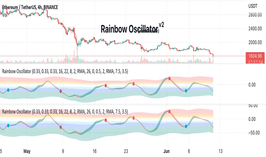
Rainbow Oscillator The Rainbow Oscillator is a technical indicator that shows prices in overbought or oversold areas. That allows you to catch the price reversal point.
---------------
FEATURES
---------------
.:: Dynamic levels ::.
The indicator levels are divided into several zones, which have a fibonacci ratio. Zones determine the overbought/oversold level. Blue and green level zones are better for buying, red and orange for selling. Dynamic levels are used as replacements for classic levels such as -100 and 100 for the CCI indicator or 30 and 70 for the RSI indicator. Dynamic levels work much better than static levels, as they are more adaptive to the current market situation.
.:: Composite oscillator (3 in 1) ::.
The main signal line of the indicator includes all three oscillators RSI, CCI, Stoch in different ratios. In the settings, you can change the proportions or completely remove one of the oscillators by setting its weight to 0
.:: CCI + RSI + Stoch ratio setting ::.
Each of the oscillators has its own weight in the calculation formula: w2 * cci ( + w1 * ( rsi - 50) + (1 - w2 - w1) * ( stoch - 50), this allows you to create the resulting oscillator from all indicators, depending on the weight of each of them. Each weight value must be between 0 and 1 so that the sum of all weights does not exceed 1.
.:: Smoothing levels and lines of the oscillator ::.
Smoothing the oscillator readings allows you to filter out the noise and get more accurate data. Level offset allows you to customize the support for inputs.
.:: Market Flat ::.
Dynamic creation of levels allows you to find in the price reversal zone, even when the price is in a flat
.:: Sources ::.
You can change the data source for the indicator to the number of longs and shorts for the selected asset. For example, BTCUSDLONGS / BTCUSDSHORTS is perfect for Bitcoin, then the oscillator will work on this data and will not use the quote price.
.:: Trend Detection ::.
The main line of the oscillator has 2 colors - green and red. Red means downtrend, green means uptrend. Trend reversal points are most often found in overbought and oversold zones.
.:: Alerts ::.
Alerts inside for next events: Buy (blue point) Sell (red point) and TrendReversal (change line color)
----------------
TRADING
—-------------
There are several possible entry points for the indicator, let's consider them all.
1) Trend reversal.
Long entry: The indicator line is in the green zone below 0 (oversold), while the line changes color from red (downward) to green (upward)
Short entry: The indicator line is in the red zone above the 0 (overbought) mark, while the line changes color from green to red.
2) Red and blue dots.
Long entry: Blue dot
Short Entry: Red Dot
I prefer to use the first trading method.
----------------
SETTINGS
----------------
.:: Trend Filter (checkbox) ::.
Use trend confirmation for red/blue dots. When enabled, the blue dot requires an uptrend, red dot requires downtrend confirmation before appearing.
.:: Use long/shorts (checkbox) ::.
Change formula to use longs and shorts positions as data source (instead of quote price)
.:: RSI weight / CCI weight / Stoch weight ::.
Weight control coefficients for RSI and CCI indicators, respectively. When you set RSI Weight = 0, equalize the combo of CCI and Stoch , when RSI Weight is zero and CCI Weight is equal to the oscillator value will be plotted
only from Stoch . Intermediate values have a high degree of measurement of each of the three oscillators in percentage terms from 0 to 100. The calculation uses the formula: w2 * cci ( + w1 * ( rsi - 50) + (1 - w2 - w1) * ( stoch - 50),
where w1 is RSI Weight and w2 is CCI Weight, Stoch weight is calculated on the fly as (1 - w2 - w1), so the sum of w1 + w2 should not exceed 1, in this case Stoch will work as opposed to CCI and RSI .
.:: Oscillograph fast and slow periods ::.
The fast period is the period for the moving average used to smooth CCI, RSI and Stoch. The slow period is the same. The fast period must always be less than the slow period.
.:: Oscillograph samples period::.
The period of smoothing the total values of indicators - creates a fast and slow main lines of the oscillator.
.:: Oscillograph samples count::.
How many times smoothing applied to source data.
.:: Oscillator samples type ::.
Smoothing line type e.g. EMA, SMA, RMA …
.:: Level period ::.
Periodically moving averages used to form the levels (zone) of the Rainbow Oscillator indicator
.:: Level offset ::.
Additional setting for shifting levels from zero points. Can be useful for absorbing levels and filtering input signals. The default is 0.
.:: Level redundant ::.
It characterizes the severity of the state at each iteration of the level of the disease. If set to 1 - the levels will not decrease when the oscillator values fall. If it has a value of 0.99 - the levels are reduced by 0.01
each has an oscillator in 1% of cases and is pressed to 0 by more aggressive ones.
.:: Level smooth samples ::.
setting allows you to set the number of strokes per level. Measuring the number of averages with the definition of the type of moving averages
.:: Level MA Type ::.
Type of moving average, average for the formation of a smoothing overbought and oversold zone
Commodity Trend Reactor [BigBeluga]
🔵 OVERVIEW
A dynamic trend-following oscillator built around the classic CCI, enhanced with intelligent price tracking and reversal signals.
Commodity Trend Reactor extends the traditional Commodity Channel Index (CCI) by integrating trend-trailing logic and reactive reversal markers. It visualizes trend direction using a trailing stop system and highlights potential exhaustion zones when CCI exceeds extreme thresholds. This dual-level system makes it ideal for both trend confirmation and mean-reversion alerts.
🔵 CONCEPTS
Based on the CCI (Commodity Channel Index) oscillator, which measures deviation from the average price.
Trend bias is determined by whether CCI is above or below user-defined thresholds.
Trailing price bands are used to lock in trend direction visually on the main chart.
Extreme values beyond ±200 are treated as potential reversal zones.
🔵 FEATURES\
CCI-Based Trend Shifts:
Triggers a bullish bias when CCI crosses above the upper threshold, and bearish when it crosses below the lower threshold.
Adaptive Trailing Stops:
In bullish mode, a trailing stop tracks the lowest price; in bearish mode, it tracks the highest.
Top & Bottom Markers:
When CCI surpasses +200 or drops below -200, it plots colored squares both on the oscillator and on price, marking potential reversal zones.
Background Highlights:
Each time a trend shift occurs, the background is softly colored (lime for bullish, orange for bearish) to highlight the change.
🔵 HOW TO USE
Use the oscillator to monitor when CCI crosses above or below threshold values to detect trend activation.
Enter trades in the direction of the trailing band once the trend bias is confirmed.
Watch for +200 and -200 square markers as warnings of potential mean reversals.
Use trailing stop areas as dynamic support/resistance to manage stop loss and exit strategies.
The background color changes offer clean confirmation of trend transitions on chart.
🔵 CONCLUSION
Commodity Trend Reactor transforms the simple CCI into a complete trend-reactive framework. With real-time trailing logic and clear reversal alerts, it serves both momentum traders and contrarian scalpers alike. Whether you’re trading breakouts or anticipating mean reversions, this indicator provides clarity and structure to your decision-making.

ADW - Volatility MapThe ADW - Volatility Map script is a tool for traders to measure and visualize the volatility of a specific asset. It uses both the Average True Range (ATR) and True Range (TR) values in combination with the Commodity Channel Index (CCI) to provide a comprehensive map of the market's volatility.
Average True Range (ATR) : ATR is a measure of market volatility. It measures the average of true price ranges over a time period. In this script, we use it to calculate the ATR-CCI which gives us a more precise measure of volatility.
True Range (TR) : TR is the greatest distance the price moved during a period. It is used in this script to calculate the TR-CCI, adding another level of detail to our volatility measurement.
Commodity Channel Index (CCI) : CCI is a versatile indicator that can be used to identify a new trend or warn of extreme conditions. We use it to scale and compare the ATR and TR values, hence providing a relative measure of volatility.
The script interprets the CCI values and provides four different conditions for both ATR and TR:
Is Low (CCI < 0)
Is High (CCI > 0)
Is Extremely Low (CCI <= -100)
Is Extremely High (CCI >= 100)
The interpretation of these conditions is displayed on the chart using colour highlighting. When the ATR or TR are low, high, extremely low, or extremely high, the script fills the chart accordingly.
In addition, the script has an option `awaitBarConfirmation` set at the beginning. If this is true, the script will only display indicators for fully formed bars, ensuring that the indicators you see are based on confirmed information.
Note: The colours for different conditions can be customized at the beginning of the script, allowing you to personalize the visual output to match your preferences.
This script is designed to provide a visually clear and immediate understanding of the market's volatility. Use it to enhance your decision-making process and adapt your trading strategy to the current market conditions.

Genesis Matrix [Loxx]Over a decade ago, the Genesis Matrix system was one of best strategies for new traders looking to learn how to really trade trends. Fast forward to 2022, a new version of Genesis Matrix has emerged using TVI, CCI, HL Channel & T3
What is T3?
The T3 moving average is an indicator of an indicator since it includes several EMAs of another EMA. Unlike any other moving average, it adds the so-called volume factor, a value between 0 and 1. Like the SMA, traders typically use this indicator to spot trends and trend reversals.
What is CCI?
The Commodity Channel Index ( CCI ) measures the current price level relative to an average price level over a given period of time. CCI is relatively high when prices are far above their average. CCI is relatively low when prices are far below their average. Using this method, CCI can be used to identify overbought and oversold levels.
Genesis matrix uses Jurik-Smoothed CCI w/ MA Deviation--a spin on regular CCI .Usually CCI is calculated as using average ( Simple Moving Average ) and mean deviation. In this version, average is replaced with well known JMA (Jurik Moving Average) instead for the smoothing phase and the deviation is replaced with variety moving average deviation. The result in this one is responsive and fast (as expected) and also it is smoother than the original CCI (as expected).
What is SSL?
Known as the SSL, the Semaphore Signal Level channel chart alert is an indicator that combines moving averages to provide you with a clear visual signal of price movement dynamics. In short, it's designed to show you when a price trend is forming. For our purposes here, SSL has been modified to allow for different moving average selection and different closing price look back periods.
What is William Blau Ergodic Tick Volume?
This is one of the techniques described by William Blau in his book "Momentum, Direction and Divergence" (1995). If you like to learn more, we advise you to read this book. His book focuses on three key aspects of trading: momentum, direction and divergence. Blau, who was an electrical engineer before becoming a trader, thoroughly examines the relationship between price and momentum in step-by-step examples. From this grounding, he then looks at the deficiencies in other oscillators and introduces some innovative techniques, including a fresh twist on Stochastics. On directional issues, he analyzes the intricacies of ADX and offers a unique approach to help define trending and non-trending periods.
William Blau's definition of TVI ergodicity is that the indictor is ergodic when periods are set to 32, 5, 1, and the signal is set to 5. Other combinations are not ergodic, according to Blau.
How to use
Long signal: All 4 indicators turn green
Short signal: All 4 indicators turn red
Included
Bar coloring

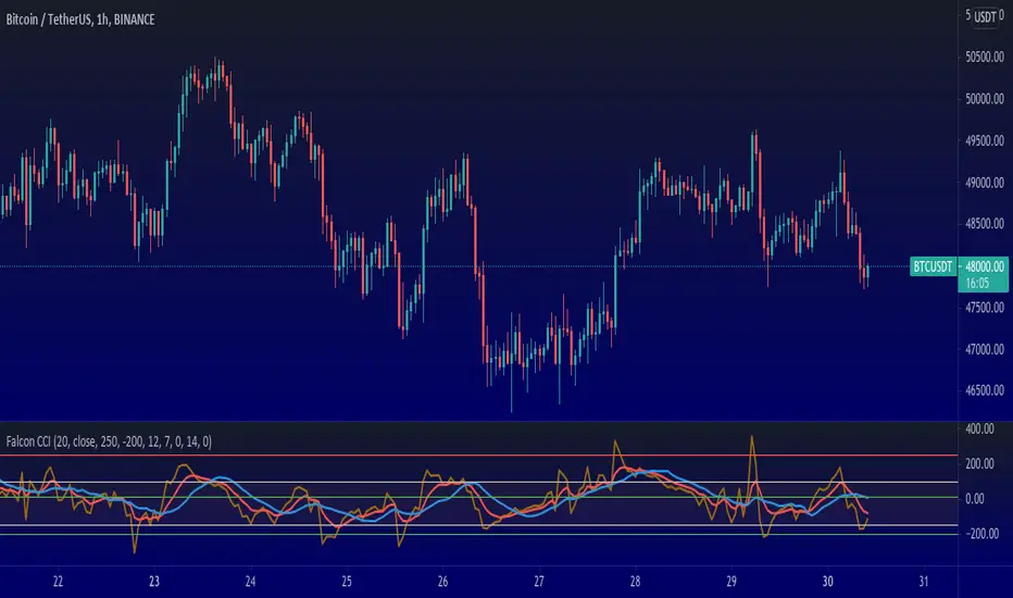
Falcon Commodity Channel IndexFalcon CCI indicator is a superb indicator for anyone who wants to dig deep and still float. The trading lifestyle requires you to be one step ahead of everyone else, while doing so, you want to manage risk, enter at correct positions and perhaps exit at correct positions too.
Exiting at correct positions is so over rated, people tend to forget that exit is as important as entry and therefore we need to make sure that we use a good indicator setup that helps us to do that.
Falcon CCI Indicator is a receipe developed by me during recent Bitcoin slump, where we really needed something more to help us get pass through ups and downs, sudden movements and volatility in the market.
This indicator is perfect even for the swing and trend traders, intra day and day traders who want a quick win, rather than invest for long term.
Here are entry and exit plans based on this indicator:-
Setup: I keep CCI at 20, MA at 14 and EMA at 7 but I change it depending on the stock or crypto. Truth is, you can play with it and find what is best for your trading setups, but once you are done, it really works.
Buy: Buy when CCI crosses above MA or EMA , but CCI should be below 50
Sell: Sell when CCI crosses below MA or EMA (You need to choose), CCI should be above 150
There can be other entry and exit based on just CCI values, and therefore I have added some max and min inputs too in the indicator, e.g. Buy when CCI is -180 and sell when CCI is 300.
Trading is a long process.
To all my friends who have lost in futures , or anywhere else in the market, don't worry, just follow the process and follow your own rules. Don't break them.
You can connect with me on Trading View, message me to discuss this further. Happy to take your questions.
P.S you can also add linear regression to this to give you certain price points, for market tops or bottoms within the time frame.
CCO_LibraryLibrary "CCO_Library"
Contrarian Crowd Oscillator (CCO) Library - Multi-oscillator consensus indicator for contrarian trading signals
@author B3AR_Trades
calculate_oscillators(rsi_length, stoch_length, cci_length, williams_length, roc_length, mfi_length, percentile_lookback, use_rsi, use_stochastic, use_williams, use_cci, use_roc, use_mfi)
Calculate normalized oscillator values
Parameters:
rsi_length (simple int) : (int) RSI calculation period
stoch_length (int) : (int) Stochastic calculation period
cci_length (int) : (int) CCI calculation period
williams_length (int) : (int) Williams %R calculation period
roc_length (int) : (int) ROC calculation period
mfi_length (int) : (int) MFI calculation period
percentile_lookback (int) : (int) Lookback period for CCI/ROC percentile ranking
use_rsi (bool) : (bool) Include RSI in calculations
use_stochastic (bool) : (bool) Include Stochastic in calculations
use_williams (bool) : (bool) Include Williams %R in calculations
use_cci (bool) : (bool) Include CCI in calculations
use_roc (bool) : (bool) Include ROC in calculations
use_mfi (bool) : (bool) Include MFI in calculations
Returns: (OscillatorValues) Normalized oscillator values
calculate_consensus_score(oscillators, use_rsi, use_stochastic, use_williams, use_cci, use_roc, use_mfi, weight_by_reliability, consensus_smoothing)
Calculate weighted consensus score
Parameters:
oscillators (OscillatorValues) : (OscillatorValues) Individual oscillator values
use_rsi (bool) : (bool) Include RSI in consensus
use_stochastic (bool) : (bool) Include Stochastic in consensus
use_williams (bool) : (bool) Include Williams %R in consensus
use_cci (bool) : (bool) Include CCI in consensus
use_roc (bool) : (bool) Include ROC in consensus
use_mfi (bool) : (bool) Include MFI in consensus
weight_by_reliability (bool) : (bool) Apply reliability-based weights
consensus_smoothing (int) : (int) Smoothing period for consensus
Returns: (float) Weighted consensus score (0-100)
calculate_consensus_strength(oscillators, consensus_score, use_rsi, use_stochastic, use_williams, use_cci, use_roc, use_mfi)
Calculate consensus strength (agreement between oscillators)
Parameters:
oscillators (OscillatorValues) : (OscillatorValues) Individual oscillator values
consensus_score (float) : (float) Current consensus score
use_rsi (bool) : (bool) Include RSI in strength calculation
use_stochastic (bool) : (bool) Include Stochastic in strength calculation
use_williams (bool) : (bool) Include Williams %R in strength calculation
use_cci (bool) : (bool) Include CCI in strength calculation
use_roc (bool) : (bool) Include ROC in strength calculation
use_mfi (bool) : (bool) Include MFI in strength calculation
Returns: (float) Consensus strength (0-100)
classify_regime(consensus_score)
Classify consensus regime
Parameters:
consensus_score (float) : (float) Current consensus score
Returns: (ConsensusRegime) Regime classification
detect_signals(consensus_score, consensus_strength, consensus_momentum, regime)
Detect trading signals
Parameters:
consensus_score (float) : (float) Current consensus score
consensus_strength (float) : (float) Current consensus strength
consensus_momentum (float) : (float) Consensus momentum
regime (ConsensusRegime) : (ConsensusRegime) Current regime classification
Returns: (TradingSignals) Trading signal conditions
calculate_cco(rsi_length, stoch_length, cci_length, williams_length, roc_length, mfi_length, consensus_smoothing, percentile_lookback, use_rsi, use_stochastic, use_williams, use_cci, use_roc, use_mfi, weight_by_reliability, detect_momentum)
Calculate complete CCO analysis
Parameters:
rsi_length (simple int) : (int) RSI calculation period
stoch_length (int) : (int) Stochastic calculation period
cci_length (int) : (int) CCI calculation period
williams_length (int) : (int) Williams %R calculation period
roc_length (int) : (int) ROC calculation period
mfi_length (int) : (int) MFI calculation period
consensus_smoothing (int) : (int) Consensus smoothing period
percentile_lookback (int) : (int) Percentile ranking lookback
use_rsi (bool) : (bool) Include RSI
use_stochastic (bool) : (bool) Include Stochastic
use_williams (bool) : (bool) Include Williams %R
use_cci (bool) : (bool) Include CCI
use_roc (bool) : (bool) Include ROC
use_mfi (bool) : (bool) Include MFI
weight_by_reliability (bool) : (bool) Apply reliability weights
detect_momentum (bool) : (bool) Calculate momentum and acceleration
Returns: (CCOResult) Complete CCO analysis results
calculate_cco_default()
Calculate CCO with default parameters
Returns: (CCOResult) CCO result with standard settings
cco_consensus_score()
Get just the consensus score with default parameters
Returns: (float) Consensus score (0-100)
cco_consensus_strength()
Get just the consensus strength with default parameters
Returns: (float) Consensus strength (0-100)
is_panic_bottom()
Check if in panic bottom condition
Returns: (bool) True if panic bottom signal active
is_euphoric_top()
Check if in euphoric top condition
Returns: (bool) True if euphoric top signal active
bullish_consensus_reversal()
Check for bullish consensus reversal
Returns: (bool) True if bullish reversal detected
bearish_consensus_reversal()
Check for bearish consensus reversal
Returns: (bool) True if bearish reversal detected
bearish_divergence()
Check for bearish divergence
Returns: (bool) True if bearish divergence detected
bullish_divergence()
Check for bullish divergence
Returns: (bool) True if bullish divergence detected
get_regime_name()
Get current regime name
Returns: (string) Current consensus regime name
get_contrarian_signal()
Get contrarian signal
Returns: (string) Current contrarian trading signal
get_position_multiplier()
Get position size multiplier
Returns: (float) Recommended position sizing multiplier
OscillatorValues
Individual oscillator values
Fields:
rsi (series float) : RSI value (0-100)
stochastic (series float) : Stochastic value (0-100)
williams (series float) : Williams %R value (0-100, normalized)
cci (series float) : CCI percentile value (0-100)
roc (series float) : ROC percentile value (0-100)
mfi (series float) : Money Flow Index value (0-100)
ConsensusRegime
Consensus regime classification
Fields:
extreme_bearish (series bool) : Extreme bearish consensus (<= 20)
moderate_bearish (series bool) : Moderate bearish consensus (20-40)
mixed (series bool) : Mixed consensus (40-60)
moderate_bullish (series bool) : Moderate bullish consensus (60-80)
extreme_bullish (series bool) : Extreme bullish consensus (>= 80)
regime_name (series string) : Text description of current regime
contrarian_signal (series string) : Contrarian trading signal
TradingSignals
Trading signals
Fields:
panic_bottom_signal (series bool) : Extreme bearish consensus with high strength
euphoric_top_signal (series bool) : Extreme bullish consensus with high strength
consensus_reversal_bullish (series bool) : Bullish consensus reversal
consensus_reversal_bearish (series bool) : Bearish consensus reversal
bearish_divergence (series bool) : Bearish price-consensus divergence
bullish_divergence (series bool) : Bullish price-consensus divergence
strong_consensus (series bool) : High consensus strength signal
CCOResult
Complete CCO calculation results
Fields:
consensus_score (series float) : Main consensus score (0-100)
consensus_strength (series float) : Consensus strength (0-100)
consensus_momentum (series float) : Rate of consensus change
consensus_acceleration (series float) : Rate of momentum change
oscillators (OscillatorValues) : Individual oscillator values
regime (ConsensusRegime) : Regime classification
signals (TradingSignals) : Trading signals
position_multiplier (series float) : Recommended position sizing multiplier

Supertrend Advance Pullback StrategyHandbook for the Supertrend Advance Strategy
1. Introduction
Purpose of the Handbook:
The main purpose of this handbook is to serve as a comprehensive guide for traders and investors who are looking to explore and harness the potential of the Supertrend Advance Strategy. In the rapidly changing financial market, having the right tools and strategies at one's disposal is crucial. Whether you're a beginner hoping to dive into the world of trading or a seasoned investor aiming to optimize and diversify your portfolio, this handbook offers the insights and methodologies you need. By the end of this guide, readers should have a clear understanding of how the Supertrend Advance Strategy works, its benefits, potential pitfalls, and practical application in various trading scenarios.
Overview of the Supertrend Advance Pullback Strategy:
At its core, the Supertrend Advance Strategy is an evolution of the popular Supertrend Indicator. Designed to generate buy and sell signals in trending markets, the Supertrend Indicator has been a favorite tool for many traders around the world. The Advance Strategy, however, builds upon this foundation by introducing enhanced mechanisms, filters, and methodologies to increase precision and reduce false signals.
1. Basic Concept:
The Supertrend Advance Strategy relies on a combination of price action and volatility to determine the potential trend direction. By assessing the average true range (ATR) in conjunction with specific price points, this strategy aims to highlight the potential starting and ending points of market trends.
2. Methodology:
Unlike the traditional Supertrend Indicator, which primarily focuses on closing prices and ATR, the Advance Strategy integrates other critical market variables, such as volume, momentum oscillators, and perhaps even fundamental data, to validate its signals. This multidimensional approach ensures that the generated signals are more reliable and are less prone to market noise.
3. Benefits:
One of the main benefits of the Supertrend Advance Strategy is its ability to filter out false breakouts and minor price fluctuations, which can often lead to premature exits or entries in the market. By waiting for a confluence of factors to align, traders using this advanced strategy can increase their chances of entering or exiting trades at optimal points.
4. Practical Applications:
The Supertrend Advance Strategy can be applied across various timeframes, from intraday trading to swing trading and even long-term investment scenarios. Furthermore, its flexible nature allows it to be tailored to different asset classes, be it stocks, commodities, forex, or cryptocurrencies.
In the subsequent sections of this handbook, we will delve deeper into the intricacies of this strategy, offering step-by-step guidelines on its application, case studies, and tips for maximizing its efficacy in the volatile world of trading.
As you journey through this handbook, we encourage you to approach the Supertrend Advance Strategy with an open mind, testing and tweaking it as per your personal trading style and risk appetite. The ultimate goal is not just to provide you with a new tool but to empower you with a holistic strategy that can enhance your trading endeavors.
2. Getting Started
Navigating the financial markets can be a daunting task without the right tools. This section is dedicated to helping you set up the Supertrend Advance Strategy on one of the most popular charting platforms, TradingView. By following the steps below, you'll be able to integrate this strategy into your charts and start leveraging its insights in no time.
Setting up on TradingView:
TradingView is a web-based platform that offers a wide range of charting tools, social networking, and market data. Before you can apply the Supertrend Advance Strategy, you'll first need a TradingView account. If you haven't set one up yet, here's how:
1. Account Creation:
• Visit TradingView's official website.
• Click on the "Join for free" or "Sign up" button.
• Follow the registration process, providing the necessary details and setting up your login credentials.
2. Navigating the Dashboard:
• Once logged in, you'll be taken to your dashboard. Here, you'll see a variety of tools, including watchlists, alerts, and the main charting window.
• To begin charting, type in the name or ticker of the asset you're interested in the search bar at the top.
3. Configuring Chart Settings:
• Before integrating the Supertrend Advance Strategy, familiarize yourself with the chart settings. This can be accessed by clicking the 'gear' icon on the top right of the chart window.
• Adjust the chart type, time intervals, and other display settings to your preference.
Integrating the Strategy into a Chart:
Now that you're set up on TradingView, it's time to integrate the Supertrend Advance Strategy.
1. Accessing the Pine Script Editor:
• Located at the top-center of your screen, you'll find the "Pine Editor" tab. Click on it.
• This is where custom strategies and indicators are scripted or imported.
2. Loading the Supertrend Advance Strategy Script:
• Depending on whether you have the script or need to find it, there are two paths:
• If you have the script: Copy the Supertrend Advance Strategy script, and then paste it into the Pine Editor.
• If searching for the script: Click on the “Indicators” icon (looks like a flame) at the top of your screen, and then type “Supertrend Advance Strategy” in the search bar. If available, it will show up in the list. Simply click to add it to your chart.
3. Applying the Strategy:
• After pasting or selecting the Supertrend Advance Strategy in the Pine Editor, click on the “Add to Chart” button located at the top of the editor. This will overlay the strategy onto your main chart window.
4. Configuring Strategy Settings:
• Once the strategy is on your chart, you'll notice a small settings ('gear') icon next to its name in the top-left of the chart window. Click on this to access settings.
• Here, you can adjust various parameters of the Supertrend Advance Strategy to better fit your trading style or the specific asset you're analyzing.
5. Interpreting Signals:
• With the strategy applied, you'll now see buy/sell signals represented on your chart. Take time to familiarize yourself with how these look and behave over various timeframes and market conditions.
3. Strategy Overview
What is the Supertrend Advance Strategy?
The Supertrend Advance Strategy is a refined version of the classic Supertrend Indicator, which was developed to aid traders in spotting market trends. The strategy utilizes a combination of data points, including average true range (ATR) and price momentum, to generate buy and sell signals.
In essence, the Supertrend Advance Strategy can be visualized as a line that moves with the price. When the price is above the Supertrend line, it indicates an uptrend and suggests a potential buy position. Conversely, when the price is below the Supertrend line, it hints at a downtrend, suggesting a potential selling point.
Strategy Goals and Objectives:
1. Trend Identification: At the core of the Supertrend Advance Strategy is the goal to efficiently and consistently identify prevailing market trends. By recognizing these trends, traders can position themselves to capitalize on price movements in their favor.
2. Reducing Noise: Financial markets are often inundated with 'noise' - short-term price fluctuations that can mislead traders. The Supertrend Advance Strategy aims to filter out this noise, allowing for clearer decision-making.
3. Enhancing Risk Management: With clear buy and sell signals, traders can set more precise stop-loss and take-profit points. This leads to better risk management and potentially improved profitability.
4. Versatility: While primarily used for trend identification, the strategy can be integrated with other technical tools and indicators to create a comprehensive trading system.
Type of Assets/Markets to Apply the Strategy:
1. Equities: The Supertrend Advance Strategy is highly popular among stock traders. Its ability to capture long-term trends makes it particularly useful for those trading individual stocks or equity indices.
2. Forex: Given the 24-hour nature of the Forex market and its propensity for trends, the Supertrend Advance Strategy is a valuable tool for currency traders.
3. Commodities: Whether it's gold, oil, or agricultural products, commodities often move in extended trends. The strategy can help in identifying and capitalizing on these movements.
4. Cryptocurrencies: The volatile nature of cryptocurrencies means they can have pronounced trends. The Supertrend Advance Strategy can aid crypto traders in navigating these often tumultuous waters.
5. Futures & Options: Traders and investors in derivative markets can utilize the strategy to make more informed decisions about contract entries and exits.
It's important to note that while the Supertrend Advance Strategy can be applied across various assets and markets, its effectiveness might vary based on market conditions, timeframe, and the specific characteristics of the asset in question. As always, it's recommended to use the strategy in conjunction with other analytical tools and to backtest its effectiveness in specific scenarios before committing to trades.
4. Input Settings
Understanding and correctly configuring input settings is crucial for optimizing the Supertrend Advance Strategy for any specific market or asset. These settings, when tweaked correctly, can drastically impact the strategy's performance.
Grouping Inputs:
Before diving into individual input settings, it's important to group similar inputs. Grouping can simplify the user interface, making it easier to adjust settings related to a specific function or indicator.
Strategy Choice:
This input allows traders to select from various strategies that incorporate the Supertrend indicator. Options might include "Supertrend with RSI," "Supertrend with MACD," etc. By choosing a strategy, the associated input settings for that strategy become available.
Supertrend Settings:
1. Multiplier: Typically, a default value of 3 is used. This multiplier is used in the ATR calculation. Increasing it makes the Supertrend line further from prices, while decreasing it brings the line closer.
2. Period: The number of bars used in the ATR calculation. A common default is 7.
EMA Settings (Exponential Moving Average):
1. Period: Defines the number of previous bars used to calculate the EMA. Common periods are 9, 21, 50, and 200.
2. Source: Allows traders to choose which price (Open, Close, High, Low) to use in the EMA calculation.
RSI Settings (Relative Strength Index):
1. Length: Determines how many periods are used for RSI calculation. The standard setting is 14.
2. Overbought Level: The threshold at which the asset is considered overbought, typically set at 70.
3. Oversold Level: The threshold at which the asset is considered oversold, often at 30.
MACD Settings (Moving Average Convergence Divergence):
1. Short Period: The shorter EMA, usually set to 12.
2. Long Period: The longer EMA, commonly set to 26.
3. Signal Period: Defines the EMA of the MACD line, typically set at 9.
CCI Settings (Commodity Channel Index):
1. Period: The number of bars used in the CCI calculation, often set to 20.
2. Overbought Level: Typically set at +100, denoting overbought conditions.
3. Oversold Level: Usually set at -100, indicating oversold conditions.
SL/TP Settings (Stop Loss/Take Profit):
1. SL Multiplier: Defines the multiplier for the average true range (ATR) to set the stop loss.
2. TP Multiplier: Defines the multiplier for the average true range (ATR) to set the take profit.
Filtering Conditions:
This section allows traders to set conditions to filter out certain signals. For example, one might only want to take buy signals when the RSI is below 30, ensuring they buy during oversold conditions.
Trade Direction and Backtest Period:
1. Trade Direction: Allows traders to specify whether they want to take long trades, short trades, or both.
2. Backtest Period: Specifies the time range for backtesting the strategy. Traders can choose from options like 'Last 6 months,' 'Last 1 year,' etc.
It's essential to remember that while default settings are provided for many of these tools, optimal settings can vary based on the market, timeframe, and trading style. Always backtest new settings on historical data to gauge their potential efficacy.
5. Understanding Strategy Conditions
Developing an understanding of the conditions set within a trading strategy is essential for traders to maximize its potential. Here, we delve deep into the logic behind these conditions, using the Supertrend Advance Strategy as our focal point.
Basic Logic Behind Conditions:
Every strategy is built around a set of conditions that provide buy or sell signals. The conditions are based on mathematical or statistical methods and are rooted in the study of historical price data. The fundamental idea is to recognize patterns or behaviors that have been profitable in the past and might be profitable in the future.
Buy and Sell Conditions:
1. Buy Conditions: Usually formulated around bullish signals or indicators suggesting upward price momentum.
2. Sell Conditions: Centered on bearish signals or indicators indicating downward price momentum.
Simple Strategy:
The simple strategy could involve using just the Supertrend indicator. Here:
• Buy: When price closes above the Supertrend line.
• Sell: When price closes below the Supertrend line.
Pullback Strategy:
This strategy capitalizes on price retracements:
• Buy: When the price retraces to the Supertrend line after a bullish signal and is supported by another bullish indicator.
• Sell: When the price retraces to the Supertrend line after a bearish signal and is confirmed by another bearish indicator.
Indicators Used:
EMA (Exponential Moving Average):
• Logic: EMA gives more weight to recent prices, making it more responsive to current price movements. A shorter-period EMA crossing above a longer-period EMA can be a bullish sign, while the opposite is bearish.
RSI (Relative Strength Index):
• Logic: RSI measures the magnitude of recent price changes to analyze overbought or oversold conditions. Values above 70 are typically considered overbought, and values below 30 are considered oversold.
MACD (Moving Average Convergence Divergence):
• Logic: MACD assesses the relationship between two EMAs of a security’s price. The MACD line crossing above the signal line can be a bullish signal, while crossing below can be bearish.
CCI (Commodity Channel Index):
• Logic: CCI compares a security's average price change with its average price variation. A CCI value above +100 may mean the price is overbought, while below -100 might signify an oversold condition.
And others...
As the strategy expands or contracts, more indicators might be added or removed. The crucial point is to understand the core logic behind each, ensuring they align with the strategy's objectives.
Logic Behind Each Indicator:
1. EMA: Emphasizes recent price movements; provides dynamic support and resistance levels.
2. RSI: Indicates overbought and oversold conditions based on recent price changes.
3. MACD: Showcases momentum and direction of a trend by comparing two EMAs.
4. CCI: Measures the difference between a security's price change and its average price change.
Understanding strategy conditions is not just about knowing when to buy or sell but also about comprehending the underlying market dynamics that those conditions represent. As you familiarize yourself with each condition and indicator, you'll be better prepared to adapt and evolve with the ever-changing financial markets.
6. Trade Execution and Management
Trade execution and management are crucial aspects of any trading strategy. Efficient execution can significantly impact profitability, while effective management can preserve capital during adverse market conditions. In this section, we'll explore the nuances of position entry, exit strategies, and various Stop Loss (SL) and Take Profit (TP) methodologies within the Supertrend Advance Strategy.
Position Entry:
Effective trade entry revolves around:
1. Timing: Enter at a point where the risk-reward ratio is favorable. This often corresponds to confirmatory signals from multiple indicators.
2. Volume Analysis: Ensure there's adequate volume to support the movement. Volume can validate the strength of a signal.
3. Confirmation: Use multiple indicators or chart patterns to confirm the entry point. For instance, a buy signal from the Supertrend indicator can be confirmed with a bullish MACD crossover.
Position Exit Strategies:
A successful exit strategy will lock in profits and minimize losses. Here are some strategies:
1. Fixed Time Exit: Exiting after a predetermined period.
2. Percentage-based Profit Target: Exiting after a certain percentage gain.
3. Indicator-based Exit: Exiting when an indicator gives an opposing signal.
Percentage-based SL/TP:
• Stop Loss (SL): Set a fixed percentage below the entry price to limit potential losses.
• Example: A 2% SL on an entry at $100 would trigger a sell at $98.
• Take Profit (TP): Set a fixed percentage above the entry price to lock in gains.
• Example: A 5% TP on an entry at $100 would trigger a sell at $105.
Supertrend-based SL/TP:
• Stop Loss (SL): Position the SL at the Supertrend line. If the price breaches this line, it could indicate a trend reversal.
• Take Profit (TP): One could set the TP at a point where the Supertrend line flattens or turns, indicating a possible slowdown in momentum.
Swing high/low-based SL/TP:
• Stop Loss (SL): For a long position, set the SL just below the recent swing low. For a short position, set it just above the recent swing high.
• Take Profit (TP): For a long position, set the TP near a recent swing high or resistance. For a short position, near a swing low or support.
And other methods...
1. Trailing Stop Loss: This dynamic SL adjusts with the price movement, locking in profits as the trade moves in your favor.
2. Multiple Take Profits: Divide the position into segments and set multiple TP levels, securing profits in stages.
3. Opposite Signal Exit: Exit when another reliable indicator gives an opposite signal.
Trade execution and management are as much an art as they are a science. They require a blend of analytical skill, discipline, and intuition. Regularly reviewing and refining your strategies, especially in light of changing market conditions, is crucial to maintaining consistent trading performance.
7. Visual Representations
Visual tools are essential for traders, as they simplify complex data into an easily interpretable format. Properly analyzing and understanding the plots on a chart can provide actionable insights and a more intuitive grasp of market conditions. In this section, we’ll delve into various visual representations used in the Supertrend Advance Strategy and their significance.
Understanding Plots on the Chart:
Charts are the primary visual aids for traders. The arrangement of data points, lines, and colors on them tell a story about the market's past, present, and potential future moves.
1. Data Points: These represent individual price actions over a specific timeframe. For instance, a daily chart will have data points showing the opening, closing, high, and low prices for each day.
2. Colors: Used to indicate the nature of price movement. Commonly, green is used for bullish (upward) moves and red for bearish (downward) moves.
Trend Lines:
Trend lines are straight lines drawn on a chart that connect a series of price points. Their significance:
1. Uptrend Line: Drawn along the lows, representing support. A break below might indicate a trend reversal.
2. Downtrend Line: Drawn along the highs, indicating resistance. A break above might suggest the start of a bullish trend.
Filled Areas:
These represent a range between two values on a chart, usually shaded or colored. For instance:
1. Bollinger Bands: The area between the upper and lower band is filled, giving a visual representation of volatility.
2. Volume Profile: Can show a filled area representing the amount of trading activity at different price levels.
Stop Loss and Take Profit Lines:
These are horizontal lines representing pre-determined exit points for trades.
1. Stop Loss Line: Indicates the level at which a trade will be automatically closed to limit losses. Positioned according to the trader's risk tolerance.
2. Take Profit Line: Denotes the target level to lock in profits. Set according to potential resistance (for long trades) or support (for short trades) or other technical factors.
Trailing Stop Lines:
A trailing stop is a dynamic form of stop loss that moves with the price. On a chart:
1. For Long Trades: Starts below the entry price and moves up with the price but remains static if the price falls, ensuring profits are locked in.
2. For Short Trades: Starts above the entry price and moves down with the price but remains static if the price rises.
Visual representations offer traders a clear, organized view of market dynamics. Familiarity with these tools ensures that traders can quickly and accurately interpret chart data, leading to more informed decision-making. Always ensure that the visual aids used resonate with your trading style and strategy for the best results.
8. Backtesting
Backtesting is a fundamental process in strategy development, enabling traders to evaluate the efficacy of their strategy using historical data. It provides a snapshot of how the strategy would have performed in past market conditions, offering insights into its potential strengths and vulnerabilities. In this section, we'll explore the intricacies of setting up and analyzing backtest results and the caveats one must be aware of.
Setting Up Backtest Period:
1. Duration: Determine the timeframe for the backtest. It should be long enough to capture various market conditions (bullish, bearish, sideways). For instance, if you're testing a daily strategy, consider a period of several years.
2. Data Quality: Ensure the data source is reliable, offering high-resolution and clean data. This is vital to get accurate backtest results.
3. Segmentation: Instead of a continuous period, sometimes it's helpful to backtest over distinct market phases, like a particular bear or bull market, to see how the strategy holds up in different environments.
Analyzing Backtest Results:
1. Performance Metrics: Examine metrics like the total return, annualized return, maximum drawdown, Sharpe ratio, and others to gauge the strategy's efficiency.
2. Win Rate: It's the ratio of winning trades to total trades. A high win rate doesn't always signify a good strategy; it should be evaluated in conjunction with other metrics.
3. Risk/Reward: Understand the average profit versus the average loss per trade. A strategy might have a low win rate but still be profitable if the average gain far exceeds the average loss.
4. Drawdown Analysis: Review the periods of losses the strategy could incur and how long it takes, on average, to recover.
9. Tips and Best Practices
Successful trading requires more than just knowing how a strategy works. It necessitates an understanding of when to apply it, how to adjust it to varying market conditions, and the wisdom to recognize and avoid common pitfalls. This section offers insightful tips and best practices to enhance the application of the Supertrend Advance Strategy.
When to Use the Strategy:
1. Market Conditions: Ideally, employ the Supertrend Advance Strategy during trending market conditions. This strategy thrives when there are clear upward or downward trends. It might be less effective during consolidative or sideways markets.
2. News Events: Be cautious around significant news events, as they can cause extreme volatility. It might be wise to avoid trading immediately before and after high-impact news.
3. Liquidity: Ensure you are trading in assets/markets with sufficient liquidity. High liquidity ensures that the price movements are more reflective of genuine market sentiment and not due to thin volume.
Adjusting Settings for Different Markets/Timeframes:
1. Markets: Each market (stocks, forex, commodities) has its own characteristics. It's essential to adjust the strategy's parameters to align with the market's volatility and liquidity.
2. Timeframes: Shorter timeframes (like 1-minute or 5-minute charts) tend to have more noise. You might need to adjust the settings to filter out false signals. Conversely, for longer timeframes (like daily or weekly charts), you might need to be more responsive to genuine trend changes.
3. Customization: Regularly review and tweak the strategy's settings. Periodic adjustments can ensure the strategy remains optimized for the current market conditions.
10. Frequently Asked Questions (FAQs)
Given the complexities and nuances of the Supertrend Advance Strategy, it's only natural for traders, both new and seasoned, to have questions. This section addresses some of the most commonly asked questions regarding the strategy.
1. What exactly is the Supertrend Advance Strategy?
The Supertrend Advance Strategy is an evolved version of the traditional Supertrend indicator. It's designed to provide clearer buy and sell signals by incorporating additional indicators like EMA, RSI, MACD, CCI, etc. The strategy aims to capitalize on market trends while minimizing false signals.
2. Can I use the Supertrend Advance Strategy for all asset types?
Yes, the strategy can be applied to various asset types like stocks, forex, commodities, and cryptocurrencies. However, it's crucial to adjust the settings accordingly to suit the specific characteristics and volatility of each asset type.
3. Is this strategy suitable for day trading?
Absolutely! The Supertrend Advance Strategy can be adjusted to suit various timeframes, making it versatile for both day trading and long-term trading. Remember to fine-tune the settings to align with the timeframe you're trading on.
4. How do I deal with false signals?
No strategy is immune to false signals. However, by combining the Supertrend with other indicators and adhering to strict risk management protocols, you can minimize the impact of false signals. Always use stop-loss orders and consider filtering trades with additional confirmation signals.
5. Do I need any prior trading experience to use this strategy?
While the Supertrend Advance Strategy is designed to be user-friendly, having a foundational understanding of trading and market analysis can greatly enhance your ability to employ the strategy effectively. If you're a beginner, consider pairing the strategy with further education and practice on demo accounts.
6. How often should I review and adjust the strategy settings?
There's no one-size-fits-all answer. Some traders adjust settings weekly, while others might do it monthly. The key is to remain responsive to changing market conditions. Regular backtesting can give insights into potential required adjustments.
7. Can the Supertrend Advance Strategy be automated?
Yes, many traders use algorithmic trading platforms to automate their strategies, including the Supertrend Advance Strategy. However, always monitor automated systems regularly to ensure they're operating as intended.
8. Are there any markets or conditions where the strategy shouldn't be used?
The strategy might generate more false signals in markets that are consolidative or range-bound. During significant news events or times of unexpected high volatility, it's advisable to tread with caution or stay out of the market.
9. How important is backtesting with this strategy?
Backtesting is crucial as it allows traders to understand how the strategy would have performed in the past, offering insights into potential profitability and areas of improvement. Always backtest any new setting or tweak before applying it to live trades.
10. What if the strategy isn't working for me?
No strategy guarantees consistent profits. If it's not working for you, consider reviewing your settings, seeking expert advice, or complementing the Supertrend Advance Strategy with other analysis methods. Remember, continuous learning and adaptation are the keys to trading success.
Other comments
Value of combining several indicators in this script and how they work together
Diversification of Signals: Just as diversifying an investment portfolio can reduce risk, using multiple indicators can offer varied perspectives on potential price movements. Each indicator can capture a different facet of the market, ensuring that traders are not overly reliant on a single data point.
Confirmation & Reduced False Signals: A common challenge with many indicators is the potential for false signals. By requiring confirmation from multiple indicators before acting, the chances of acting on a false signal can be significantly reduced.
Flexibility Across Market Conditions: Different indicators might perform better under different market conditions. For example, while moving averages might excel in trending markets, oscillators like RSI might be more useful during sideways or range-bound conditions. A mashup strategy can potentially adapt better to varying market scenarios.
Comprehensive Analysis: With multiple indicators, traders can gauge trend strength, momentum, volatility, and potential market reversals all at once, providing a holistic view of the market.
How do the different indicators in the Supertrend Advance Strategy work together?
Supertrend: This is primarily a trend-following indicator. It provides traders with buy and sell signals based on the volatility of the price. When combined with other indicators, it can filter out noise and give more weight to strong, confirmed trends.
EMA (Exponential Moving Average): EMA gives more weight to recent price data. It can be used to identify the direction and strength of a trend. When the price is above the EMA, it's generally considered bullish, and vice versa.
RSI (Relative Strength Index): An oscillator that measures the magnitude of recent price changes to evaluate overbought or oversold conditions. By cross-referencing with other indicators like EMA or MACD, traders can spot potential reversals or confirmations of a trend.
MACD (Moving Average Convergence Divergence): This indicator identifies changes in the strength, direction, momentum, and duration of a trend in a stock's price. When the MACD line crosses above the signal line, it can be a bullish sign, and when it crosses below, it can be bearish. Pairing MACD with Supertrend can provide dual confirmation of a trend.
CCI (Commodity Channel Index): Initially developed for commodities, CCI can indicate overbought or oversold conditions. It can be used in conjunction with other indicators to determine entry and exit points.
In essence, the synergy of these indicators provides a balanced, comprehensive approach to trading. Each indicator offers its unique lens into market conditions, and when they align, it can be a powerful indication of a trading opportunity. This combination not only reduces the potential drawbacks of each individual indicator but leverages their strengths, aiming for more consistent and informed trading decisions.
Backtesting and Default Settings
• This indicator has been optimized to be applied for 1 hour-charts. However, the underlying principles of this strategy are supply and demand in the financial markets and the strategy can be applied to all timeframes. Daytraders can use the 1min- or 5min charts, swing-traders can use the daily charts.
• This strategy has been designed to identify the most promising, highest probability entries and trades for each stock or other financial security.
• The combination of the qualifiers results in a highly selective strategy which only considers the most promising swing-trading entries. As a result, you will normally only find a low number of trades for each stock or other financial security per year in case you apply this strategy for the daily charts. Shorter timeframes will result in a higher number of trades / year.
• Consequently, traders need to apply this strategy for a full watchlist rather than just one financial security.
• Default properties: RSI on (length 14, RSI buy level 50, sell level 50), EMA, RSI, MACD on, type of strategy pullback, SL/TP type: ATR (length 10, factor 3), trade direction both, quantity 5, take profit swing hl 5.1, highest / lowest lookback 2, enable ATR trail (ATR length 10, SL ATR multiplier 1.4, TP multiplier 2.1, lookback = 4, trade direction = both).
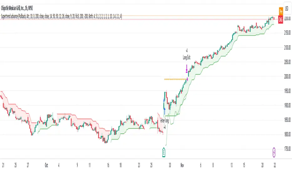
Supply and Demand Zone ConfirmationHello traders and investors,
Today, I am going to share an indicator that I made by mixing RSI and CCI in different timeframe. You can use this indicator in various ways, however the best possible way I would recommend you to use it is to combine it with price action. I would suggest to play with, so you can decide if it works the best for you.
The whole purpose of making this indicator was to eliminate confusion around different indicators for overbought and oversold and many other headaches. You use price action and you are looking for confirmation to see there is a PRZ? here is your indicator. I found there are certain patterns with CCI and RSI in higher timeframe which helps to find the PRZ and I made this indicator with it.
You can choose to use this indicator in different timeframe. But you have to consider, the lower timeframe you'll go, you will get more signals but the effectiveness goes down with it. Also, if you are willing to change the time frame, You have to change some settings as well which I'll get into it in a moment.
The default settings are for 30min timeframe with these settings.
ibb.co
In case you would like to go to 15min time frame, here is the suggested changes in the setting.
ibb.co
I would suggest to play with different timeframe to find the suitable setting for the pairs you would like to trade. The main goal is you have to choose first CCI one timeframe higher ( if you are in 5min chart, first CCI should be at least 15 or 30min) and the second CCI one timeframe higher than first CCI (if you choose 15min for first CCI, go with 1hr for second CCI). And lastly, RSI can be variable but it is suggested to be at least as low as first CCI timeframe.
Lastly, you have to consider nothing in this script is a financial advice, it is only to help you improve your trading style by making other indicators as simple as possible.

***CILGIN INDIKATOR***ÇILGIN INDICATOR – User Guide
OVERVIEW
ÇILGIN INDICATOR is a multi-layer trend and momentum confirmation tool designed for discretionary traders.
It combines Relative RSI, EMA structure, SuperTrend logic, Momentum, and optional CCI & ADX filters into a single visual system.
Purpose:
Filter market noise, confirm trend strength, and highlight high-probability Buy / Sell zones.
The indicator works on all symbols and all timeframes.
RELATIVE RSI & MOMENTUM
The indicator can work in two modes:
NORMAL MODE (Formula OFF)
RSI is calculated directly from the chart symbol.
FORMULA MODE (Formula ON)
RSI is calculated from a relative price formula:
Base Symbol / Denominator 1 / Denominator 2
This allows relative strength analysis against indices, sectors, or benchmarks.
RSI SIGNAL LOGIC
RSI Signal Line = SMA of RSI
RSI 50 Level = Trend bias reference
BUY SIGNAL
RSI crosses above the signal line
Optional: RSI must also cross above 50 (Double Confirmation)
SELL SIGNAL
RSI crosses below the signal line
Optional: RSI must also cross below 50
Small arrows on the chart represent RSI-based Buy and Sell signals.
EMA STRUCTURE
Five adaptive EMAs are plotted: EMA 1
EMA 5
EMA 21
EMA 50
EMA 100
EMA lengths automatically adapt to timeframe speed.
EMA BUY LOGIC
Fast EMA crosses above any slower EMA.
EMA SELL LOGIC
Fast EMA crosses below any slower EMA.
EMAs define:
Trend direction
Dynamic support and resistance
Momentum shifts
SUPERTREND SYSTEM
A custom ATR-based SuperTrend is used.
Features:
Optional candle wick usage
Dynamic trailing stop
Visual Buy / Sell labels
SUPERTREND BUY
Trend flips from bearish to bullish.
SUPERTREND SELL
Trend flips from bullish to bearish.
Colored zones visualize the active trend direction.
STRONG BUY & STRONG SELL SIGNALS
A Strong Signal is generated only when multiple conditions agree.
STRONG BUY
RSI Buy Signal
SuperTrend Buy Signal
Optional CCI Filter confirmation
Optional ADX Filter confirmation
STRONG SELL
RSI Sell Signal
SuperTrend Sell Signal
Optional CCI Filter confirmation
Optional ADX Filter confirmation
Strong signals are displayed as large labeled markers: “STRONG BUY”
“STRONG SELL”
Designed for trend-following entries, not market noise.
CCI & ADX FILTERS (OPTIONAL)
CCI FILTER
Buy allowed only if CCI > 0
Sell allowed only if CCI < 0
ADX FILTER
ADX must be above minimum level
Direction confirmed using +DI and -DI
These filters help avoid sideways markets and weak trends.
INFORMATION PANELS
PANEL A (Top Right)
Daily percentage change
Weekly percentage change
Monthly percentage change
Daily volume (millions)
PANEL B (Bottom Right)
Relative RSI value
RSI signal value
Relative momentum
Market status (Bull / Bear)
Provides instant market context without extra indicators.
ALERTS
Built-in alerts are available for:
STRONG BUY
STRONG SELL
Suitable for automation and watchlist monitoring.
BEST PRACTICES
Use Formula Mode for relative strength analysis
Enable CCI & ADX filters on higher timeframes
Combine signals with price action and key levels
Do not use as a standalone trading system
DISCLAIMER
This indicator is a decision-support tool and does not provide financial advice.
Always manage risk and confirm signals with your own analysis.

Scout Regiment - Signal📊 中文版
指标简介
Buy/Sell Signal 多维度交易信号指标
这是一个结合了EMA趋势过滤、CCI动量指标和RSI背景环境的多维度交易信号系统。通过三重过滤机制,帮助交易者在合适的市场环境中捕捉高质量的买卖信号。
核心特点
✅ 趋势过滤:使用233周期EMA确保顺势交易
✅ 动量确认:CCI(33)穿越信号作为入场触发
✅ 背景过滤:RSI(13)环境判断,避免同一背景重复信号
✅ 智能去重:每个RSI背景周期内只标记首次信号
✅ 清晰标识:三角形标记配合颜色区分买卖方向
使用说明
信号逻辑:
做多信号 (Buy):
收盘价 > EMA233(确认上升趋势)
CCI33向上穿越20(动量转强)
情况1:在RSI红色背景中首次出现
情况2:在RSI绿色背景中出现
做空信号 (Sell):
收盘价 < EMA233(确认下降趋势)
CCI33向下穿越80(动量转弱)
情况1:在RSI绿色背景中首次出现
情况2:在RSI红色背景中出现
参数设置
EMA过滤长度:默认233,用于判断主趋势方向
CCI长度:默认33,控制动量指标灵敏度
RSI长度:默认13,用于背景环境判断
重要提示
⚠️ 信号出现后不要立即下单!请务必检查:
CCI中期是否出现"浪子回头"形态
OBV成交量状态是否配合
RSI是否成功穿越50中线
结合其他技术分析工具综合判断
💡 建议配合使用:
支撑阻力位分析
成交量指标(如OBV)
更大周期的趋势确认
📈 English Version
Indicator Overview
Buy/Sell Signal - Multi-Dimensional Trading Signal System
This is a comprehensive trading signal system that combines EMA trend filtering, CCI momentum indicator, and RSI background environment. Through a triple-layer filtering mechanism, it helps traders capture high-quality buy and sell signals in appropriate market conditions.
Key Features
✅ Trend Filter: 233-period EMA ensures trend-following trades
✅ Momentum Confirmation: CCI(33) crossover signals as entry triggers
✅ Background Filter: RSI(13) environment detection to avoid duplicate signals
✅ Smart Deduplication: Only first signal per RSI background cycle
✅ Clear Visualization: Triangle markers with color-coded direction
How to Use
Signal Logic:
Buy Signal:
Close > EMA233 (confirms uptrend)
CCI33 crosses above 20 (momentum strengthens)
Case 1: First occurrence in RSI red background
Case 2: Occurs in RSI green background
Sell Signal:
Close < EMA233 (confirms downtrend)
CCI33 crosses below 80 (momentum weakens)
Case 1: First occurrence in RSI green background
Case 2: Occurs in RSI red background
Parameter Settings
EMA Filter Length: Default 233, for main trend direction
CCI Length: Default 33, controls momentum sensitivity
RSI Length: Default 13, for background environment detection
Important Notes
⚠️ DO NOT enter trades immediately after signal appears! Always check:
Whether CCI shows a "reversal" pattern in medium-term
OBV volume status confirmation
Whether RSI successfully crosses the 50 midline
Combine with other technical analysis tools
💡 Recommended to Use With:
Support/Resistance analysis
Volume indicators (such as OBV)
Higher timeframe trend confirmation
Risk Disclaimer
This indicator is for reference only and does not constitute investment advice. Trading involves risk. Please conduct thorough analysis and use proper risk management before making any trading decisions.
适合交易者类型 / Suitable For:
波段交易者 / Swing Traders
日内交易者 / Day Traders
趋势跟踪者 / Trend Followers
适用市场 / Applicable Markets:
股票 / Stocks
外汇 / Forex
加密货币 / Crypto
期货 / Futures
