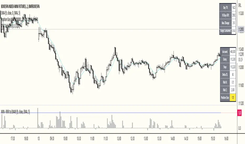
ATR Table 2.0ATR Table 2.0
This script was created in order to display a table that "calculates" how far the price can go on the current day .
The script is a table with 3 lines that calculates:
First Line - Day TR: The True Range of the current day ( - , including an Opening GAP if it exists);
Second Line - 10 Day ATR: The Average True Range of the asset (including Opening GAPs) for the last 10 days;
Third LIne - Range Consumed: How much of the 10 Day ATR it was consumed on the current day.
Example of how to use the information on the table and the understanding of it's purpose:
1) Supose you are day trading an asset that, during the last 10 days, have moved around $1.00 a day - This is the 10 Day ATR.
2) On this day, after 2 hours of the opening market, the price have already moved $0.50 (supose that it has moved $0.30 up and $0.35 down from the close of the prior day and the price is now near the close of the prior day).
3) In this situation, knowing that the price often moves around $1.00 a day, and knowing that it already moved $0.65 ($0.30 up and $0.35 down based on the close of the prior day), you may pay attention when the price breaksthrough the max or the min of the day, cause it can still move $0.35 in that direction ($1.00 - $0.65).
----------------------------------------------
ATR Table 2.0
Esse script foi criado para disponibilizar uma tabela que "calcula" quanto o preço pode andar ainda no dia em questão .
O script é uma tabela com 3 linhas que calcula:
Primeira Linha - TR do Dia: O Range Verdadeira do dia em questão ( - , incluindo GAP de Abertura se for o caso);
Segunda Linha - ATR de 10 Dias: A média do Range Verdadeira do ativo (incluindo GAPs de abertura) dos últimos 10 dias;
Terceira Linha - Range Consumido: O quanto do ATR de 10dias já foi consumido no dia em questão.
Exemplo de como usar essa informação na tabela e o entendimento do seu propósito:
1) Suponha que você está realizando day trade de um ativo que, durante os últimos 10 dias, se move em torno de $1.00 por dia. Esse é o ATR de 10 dias.
2) Nesse dia, após 2 horas da abertura do pregão, o preço já se moveu $.050 (suponhamos que ele tenha se moveu $0.30 para cima e $0.35 para baixo a partir do fechamento do dia anterior e agora o preço está próximo do fechamento do dia anterior).
3) Nessa situação, sabendo que o preço se move por volta de $1.00 por dia, e sabendo que ele já se moveu $0.65 ($0.30 pra cima e $0.35 pra baixo a partir do fechamento do dia anterior), você deve se atentar para quando o preço romper a máxima ou a mínima do dia, pois ele pode se mover ainda $.035 na direção do rompimento ($1.00 - $0.65).
Pesquisar nos scripts por "美国夏威夷+prime公司"
My exponential moving averages - Suri's EMAs
It's not an indication of anything here, it's just part of my operating in a simple and summarized way, I hope it helps someone.
Suri's EMA's indicator is nothing more than a set of exponential moving averages (EMA). They are 12, 26, 50 and 200.
Attention to the use of the indicator, it is just an INDICATOR, it should not be taken as the main point of your entry, but to guide you in your entries in favor of the trend, whether intra-day or swing.
Created for clear, monochrome screens. Make your adjustments.
Color condition, candles turn green when their close is above EMA 12 and 26.
Color condition, candles turn red when their close is below EMA 12 and 26.
Condition for colors, MME12,26,50 and 200 will turn green with price working above it.
Condition for colors, MME12, 26, 50 and 200 will turn red with price working below it.
Indication for use in time-frames = 5m, 15m, 60m, 240m. (higher hit rates)
How to use the indicator, MME 12 and 26, are the most important and led you to more entries, but we should not only consider them, we have to analyze the whole context to then make a decision.
Indicator was nicknamed by me by "Pullback Pick", it works in a simple way:
In an uptrend or downtrend, the price usually tends to return in the averages or the averages go up to the price, that being said, it is easy to observe that where the price returns would be a pullback from the last movement, so when returning to the averages, the candle that shows strength in favor of this trend, in the EMA's region, becomes a possible entry, with its stop below or above this "pullback" formed, because the stop goes there, because usually when the price returns on the EMAs they tend to to hold and replay the price in favor of the trend.
My observations:
I like to enter when the price returns to the averages smoothly, without much movement, when it touches the average 12 or 26 it is an entry, but an entry without confirmation, the gain is greater, but the chance of being stopped is higher, I like it when the price is close to the 12 and 26 averages and leaves a small candle or doji on this pullback, my entry goes to the breakout of this candle and the stop behind the candle.
THERE IS NO MIRACLE, THERE IS NO 100% HIT RATE, SO USE STOP.
Aaaaaaaaaa I was forgetting.... and the target???
As it is a trend following setup, it is cool to leave a trailing stop or update the stop as new bottoms or tops are formed.
Targeting in 1v1 is good, setup pays a lot!
Targeting in 2x1 is too good, setup pays well!
Making a target in 3x1 is more than good, setup pays sometimes, then from now on, it depends on where you are entering this "PULLBACK", if it is in the first wave, in the second, if you are going to lateralize, the market is SOVEREIGN, put in the pocket that is no longer on the market, oh it's yours!
That's it, doubts, send it there, suggestion, opinion, whatever you want.
Added a symbol at the crossing of the 12 and 26 moving averages.
I am so sorry, but i dont speak english, use google translate.
Português.
Não se trata de indicação de nada aqui, é apenas parte do meu operacional de maneira simples e resumida, espero que ajude alguém.
Indicador Suri's EMA's, nada mais é do que um conjunto de médias móveis exponenciais(MME). São elas 12, 26, 50 e 200.
Atenção para o uso do indicador, ele é apenas um INDICADOR, não deve ser tomado como o ponto principal de sua entrada, mas sim de te balizar nas suas entradas a favor da tendência, seja ela intra-day ou swing.
Criado para telas claras e monocromáticas. Façam seus ajustes.
Condição para as cores, candles ficam verdes quando o fechamento dele é acima das MME 12 e 26.
Condição para as cores, candles ficam vermelhos quando o fechamento dele é abaixo das MME 12 e 26.
Condição para as cores, MME12,26,50 e 200 ficará verde com preço trabalhando acima dela.
Condição para as cores, MME12, 26, 50 e 200 ficará vermelho com preço trabalhando abaixo dela.
Indicação para uso nos time-frame = 5m, 15m, 60m, 240m.(taxas de acerto maior)
Como utilizar o indicador, MME 12 e 26, são as mais importantes e te levaram a mais entradas, porém não devemos levar apenas elas em consideração, temos que analisar todo o contexto para então tomar decisão.
Indicador foi apelidado por mim por " Pega Pullback", ele funciona de uma maneira simples:
Em tendência de alta ou de baixa, o preço geralmente tende a retornar nas médias ou as médias irem até o preço, dito isso é fácil de se observar que onde o preço retorna seria um pullback do último movimento, portanto ao retornar nas médias, o candle que mostra força a favor dessa tendência, na região das EMA's, se torna uma possível entrada, com o seu stop abaixo ou acima desse "pullback" formado, porque o stop vai nesse local, porque geralmente quando o preço retorna nas EMAs elas tendem a segurar e voltar a jogar o preço a favor da tendência.
Minhas observações:
Eu gosto de entrar quando o preço retorna nas médias de maneira suave, sem muito movimento, quando toca na média 12 ou 26 é uma entrada, porém uma entrada sem confirmação, o ganho é maior, porém a chance de ser stopado é mais alta, eu gosto quando o preço fica perto das médias 12 e 26 e deixa um candle pequeno ou doji nesse pullback, minha entrada vai no rompimento desse candle e o stop atrás do candle.
Não existe MILAGRE, NÃO EXISTE TAXA DE ACERTO DE 100%, POR ISSO USE STOP.
Aaaaaaaaaa ia me esquecendo.... e o alvo???
Por ser um setup seguidor de tendência, o legal é deixar um trailing stop ou ir atualizando o stop conforme novos fundos ou topos são formados.
Realizar alvo no 1x1 é bom, setup paga muito!
Realizar alvo no 2x1 é bom de mais, setup paga bem!
Realizar alvo no 3x1 é mais do que bom, setup paga as vezes, ai daqui pra frente, depende de onde você está entrando nesse "PULLBACK", se é na primeira onda, na segunda, se vai lateralizar, o mercado é SOBERANO, põe no bolso que não é mais do mercado, ai é teu!
É isso, dúvidas, manda ai, sugestão, opinião, o que quiser.
Adicionado um símbolo no cruzamento das médias móveis 12 e 26.

Estocastoco Lento - DTOperacional criado pelo Jean Lira - Trader.
Basicamente busca uma situação de confirmação de exaustão com o indicador estocastico.
Na primeira barra de reversão do movimento, e com o sinal forte do estocastico Lento, no periodo de 5.
Gerenciamento de risco com e sem parcial.

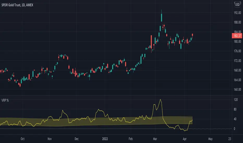
Volatility Risk Premium GOLD & SILVER 1.0ENGLISH
This indicator (V-R-P) calculates the (one month) Volatility Risk Premium for GOLD and SILVER.
V-R-P is the premium hedgers pay for over Realized Volatility for GOLD and SILVER options.
The premium stems from hedgers paying to insure their portfolios, and manifests itself in the differential between the price at which options are sold (Implied Volatility) and the volatility GOLD and SILVER ultimately realize (Realized Volatility).
I am using 30-day Implied Volatility (IV) and 21-day Realized Volatility (HV) as the basis for my calculation, as one month of IV is based on 30 calendaristic days and one month of HV is based on 21 trading days.
At first, the indicator appears blank and a label instructs you to choose which index you want the V-R-P to plot on the chart. Use the indicator settings (the sprocket) to choose one of the precious metals (or both).
Together with the V-R-P line, the indicator will show its one year moving average within a range of +/- 15% (which you can change) for benchmarking purposes. We should consider this range the “normalized” V-R-P for the actual period.
The Zero Line is also marked on the indicator.
Interpretation
When V-R-P is within the “normalized” range, … well... volatility and uncertainty, as it’s seen by the option market, is “normal”. We have a “premium” of volatility which should be considered normal.
When V-R-P is above the “normalized” range, the volatility premium is high. This means that investors are willing to pay more for options because they see an increasing uncertainty in markets.
When V-R-P is below the “normalized” range but positive (above the Zero line), the premium investors are willing to pay for risk is low, meaning they see decreasing uncertainty and risks in the market, but not by much.
When V-R-P is negative (below the Zero line), we have COMPLACENCY. This means investors see upcoming risk as being lower than what happened in the market in the recent past (within the last 30 days).
CONCEPTS :
Volatility Risk Premium
The volatility risk premium (V-R-P) is the notion that implied volatility (IV) tends to be higher than realized volatility (HV) as market participants tend to overestimate the likelihood of a significant market crash.
This overestimation may account for an increase in demand for options as protection against an equity portfolio. Basically, this heightened perception of risk may lead to a higher willingness to pay for these options to hedge a portfolio.
In other words, investors are willing to pay a premium for options to have protection against significant market crashes even if statistically the probability of these crashes is lesser or even negligible.
Therefore, the tendency of implied volatility is to be higher than realized volatility, thus V-R-P being positive.
Realized/Historical Volatility
Historical Volatility (HV) is the statistical measure of the dispersion of returns for an index over a given period of time.
Historical volatility is a well-known concept in finance, but there is confusion in how exactly it is calculated. Different sources may use slightly different historical volatility formulas.
For calculating Historical Volatility I am using the most common approach: annualized standard deviation of logarithmic returns, based on daily closing prices.
Implied Volatility
Implied Volatility (IV) is the market's forecast of a likely movement in the price of the index and it is expressed annualized, using percentages and standard deviations over a specified time horizon (usually 30 days).
IV is used to price options contracts where high implied volatility results in options with higher premiums and vice versa. Also, options supply and demand and time value are major determining factors for calculating Implied Volatility.
Implied Volatility usually increases in bearish markets and decreases when the market is bullish.
For determining GOLD and SILVER implied volatility I used their volatility indices: GVZ and VXSLV (30-day IV) provided by CBOE.
Warning
Please be aware that because CBOE doesn’t provide real-time data in Tradingview, my V-R-P calculation is also delayed, so you shouldn’t use it in the first 15 minutes after the opening.
This indicator is calibrated for a daily time frame.
----------------------------------------------------------------------
ESPAŇOL
Este indicador (V-R-P) calcula la Prima de Riesgo de Volatilidad (de un mes) para GOLD y SILVER.
V-R-P es la prima que pagan los hedgers sobre la Volatilidad Realizada para las opciones de GOLD y SILVER.
La prima proviene de los hedgers que pagan para asegurar sus carteras y se manifiesta en el diferencial entre el precio al que se venden las opciones (Volatilidad Implícita) y la volatilidad que finalmente se realiza en el ORO y la PLATA (Volatilidad Realizada).
Estoy utilizando la Volatilidad Implícita (IV) de 30 días y la Volatilidad Realizada (HV) de 21 días como base para mi cálculo, ya que un mes de IV se basa en 30 días calendario y un mes de HV se basa en 21 días de negociación.
Al principio, el indicador aparece en blanco y una etiqueta le indica que elija qué índice desea que el V-R-P represente en el gráfico. Use la configuración del indicador (la rueda dentada) para elegir uno de los metales preciosos (o ambos).
Junto con la línea V-R-P, el indicador mostrará su promedio móvil de un año dentro de un rango de +/- 15% (que puede cambiar) con fines de evaluación comparativa. Deberíamos considerar este rango como el V-R-P "normalizado" para el período real.
La línea Cero también está marcada en el indicador.
Interpretación
Cuando el V-R-P está dentro del rango "normalizado",... bueno... la volatilidad y la incertidumbre, como las ve el mercado de opciones, es "normal". Tenemos una “prima” de volatilidad que debería considerarse normal.
Cuando V-R-P está por encima del rango "normalizado", la prima de volatilidad es alta. Esto significa que los inversores están dispuestos a pagar más por las opciones porque ven una creciente incertidumbre en los mercados.
Cuando el V-R-P está por debajo del rango "normalizado" pero es positivo (por encima de la línea Cero), la prima que los inversores están dispuestos a pagar por el riesgo es baja, lo que significa que ven una disminución, pero no pronunciada, de la incertidumbre y los riesgos en el mercado.
Cuando V-R-P es negativo (por debajo de la línea Cero), tenemos COMPLACENCIA. Esto significa que los inversores ven el riesgo próximo como menor que lo que sucedió en el mercado en el pasado reciente (en los últimos 30 días).
CONCEPTOS :
Prima de Riesgo de Volatilidad
La Prima de Riesgo de Volatilidad (V-R-P) es la noción de que la Volatilidad Implícita (IV) tiende a ser más alta que la Volatilidad Realizada (HV) ya que los participantes del mercado tienden a sobrestimar la probabilidad de una caída significativa del mercado.
Esta sobreestimación puede explicar un aumento en la demanda de opciones como protección contra una cartera de acciones. Básicamente, esta mayor percepción de riesgo puede conducir a una mayor disposición a pagar por estas opciones para cubrir una cartera.
En otras palabras, los inversores están dispuestos a pagar una prima por las opciones para tener protección contra caídas significativas del mercado, incluso si estadísticamente la probabilidad de estas caídas es menor o insignificante.
Por lo tanto, la tendencia de la Volatilidad Implícita es de ser mayor que la Volatilidad Realizada, por lo cual el V-R-P es positivo.
Volatilidad Realizada/Histórica
La Volatilidad Histórica (HV) es la medida estadística de la dispersión de los rendimientos de un índice durante un período de tiempo determinado.
La Volatilidad Histórica es un concepto bien conocido en finanzas, pero existe confusión sobre cómo se calcula exactamente. Varias fuentes pueden usar fórmulas de Volatilidad Histórica ligeramente diferentes.
Para calcular la Volatilidad Histórica, utilicé el enfoque más común: desviación estándar anualizada de rendimientos logarítmicos, basada en los precios de cierre diarios.
Volatilidad Implícita
La Volatilidad Implícita (IV) es la previsión del mercado de un posible movimiento en el precio del índice y se expresa anualizada, utilizando porcentajes y desviaciones estándar en un horizonte de tiempo específico (generalmente 30 días).
IV se utiliza para cotizar contratos de opciones donde la alta Volatilidad Implícita da como resultado opciones con primas más altas y viceversa. Además, la oferta y la demanda de opciones y el valor temporal son factores determinantes importantes para calcular la Volatilidad Implícita.
La Volatilidad Implícita generalmente aumenta en los mercados bajistas y disminuye cuando el mercado es alcista.
Para determinar la Volatilidad Implícita de GOLD y SILVER utilicé sus índices de volatilidad: GVZ y VXSLV (30 días IV) proporcionados por CBOE.
Precaución
Tenga en cuenta que debido a que CBOE no proporciona datos en tiempo real en Tradingview, mi cálculo de V-R-P también se retrasa, y por este motivo no se recomienda usar en los primeros 15 minutos desde la apertura.
Este indicador está calibrado para un marco de tiempo diario.
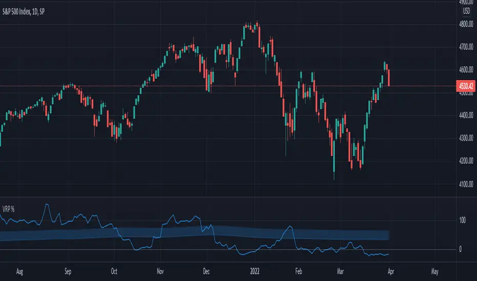
Volatility Risk Premium (VRP) 1.0ENGLISH
This indicator (V-R-P) calculates the (one month) Volatility Risk Premium for S&P500 and Nasdaq-100.
V-R-P is the premium hedgers pay for over Realized Volatility for S&P500 and Nasdaq-100 index options.
The premium stems from hedgers paying to insure their portfolios, and manifests itself in the differential between the price at which options are sold (Implied Volatility) and the volatility the S&P500 and Nasdaq-100 ultimately realize (Realized Volatility).
I am using 30-day Implied Volatility (IV) and 21-day Realized Volatility (HV) as the basis for my calculation, as one month of IV is based on 30 calendaristic days and one month of HV is based on 21 trading days.
At first, the indicator appears blank and a label instructs you to choose which index you want the V-R-P to plot on the chart. Use the indicator settings (the sprocket) to choose one of the indices (or both).
Together with the V-R-P line, the indicator will show its one year moving average within a range of +/- 15% (which you can change) for benchmarking purposes. We should consider this range the “normalized” V-R-P for the actual period.
The Zero Line is also marked on the indicator.
Interpretation
When V-R-P is within the “normalized” range, … well... volatility and uncertainty, as it’s seen by the option market, is “normal”. We have a “premium” of volatility which should be considered normal.
When V-R-P is above the “normalized” range, the volatility premium is high. This means that investors are willing to pay more for options because they see an increasing uncertainty in markets.
When V-R-P is below the “normalized” range but positive (above the Zero line), the premium investors are willing to pay for risk is low, meaning they see decreasing uncertainty and risks in the market, but not by much.
When V-R-P is negative (below the Zero line), we have COMPLACENCY. This means investors see upcoming risk as being lower than what happened in the market in the recent past (within the last 30 days).
CONCEPTS:
Volatility Risk Premium
The volatility risk premium (V-R-P) is the notion that implied volatility (IV) tends to be higher than realized volatility (HV) as market participants tend to overestimate the likelihood of a significant market crash.
This overestimation may account for an increase in demand for options as protection against an equity portfolio. Basically, this heightened perception of risk may lead to a higher willingness to pay for these options to hedge a portfolio.
In other words, investors are willing to pay a premium for options to have protection against significant market crashes even if statistically the probability of these crashes is lesser or even negligible.
Therefore, the tendency of implied volatility is to be higher than realized volatility, thus V-R-P being positive.
Realized/Historical Volatility
Historical Volatility (HV) is the statistical measure of the dispersion of returns for an index over a given period of time.
Historical volatility is a well-known concept in finance, but there is confusion in how exactly it is calculated. Different sources may use slightly different historical volatility formulas.
For calculating Historical Volatility I am using the most common approach: annualized standard deviation of logarithmic returns, based on daily closing prices.
Implied Volatility
Implied Volatility (IV) is the market's forecast of a likely movement in the price of the index and it is expressed annualized, using percentages and standard deviations over a specified time horizon (usually 30 days).
IV is used to price options contracts where high implied volatility results in options with higher premiums and vice versa. Also, options supply and demand and time value are major determining factors for calculating Implied Volatility.
Implied Volatility usually increases in bearish markets and decreases when the market is bullish.
For determining S&P500 and Nasdaq-100 implied volatility I used their volatility indices: VIX and VXN (30-day IV) provided by CBOE.
Warning
Please be aware that because CBOE doesn’t provide real-time data in Tradingview, my V-R-P calculation is also delayed, so you shouldn’t use it in the first 15 minutes after the opening.
This indicator is calibrated for a daily time frame.
ESPAŇOL
Este indicador (V-R-P) calcula la Prima de Riesgo de Volatilidad (de un mes) para S&P500 y Nasdaq-100.
V-R-P es la prima que pagan los hedgers sobre la Volatilidad Realizada para las opciones de los índices S&P500 y Nasdaq-100.
La prima proviene de los hedgers que pagan para asegurar sus carteras y se manifiesta en el diferencial entre el precio al que se venden las opciones (Volatilidad Implícita) y la volatilidad que finalmente se realiza en el S&P500 y el Nasdaq-100 (Volatilidad Realizada).
Estoy utilizando la Volatilidad Implícita (IV) de 30 días y la Volatilidad Realizada (HV) de 21 días como base para mi cálculo, ya que un mes de IV se basa en 30 días calendario y un mes de HV se basa en 21 días de negociación.
Al principio, el indicador aparece en blanco y una etiqueta le indica que elija qué índice desea que el V-R-P represente en el gráfico. Use la configuración del indicador (la rueda dentada) para elegir uno de los índices (o ambos).
Junto con la línea V-R-P, el indicador mostrará su promedio móvil de un año dentro de un rango de +/- 15% (que puede cambiar) con fines de evaluación comparativa. Deberíamos considerar este rango como el V-R-P "normalizado" para el período real.
La línea Cero también está marcada en el indicador.
Interpretación
Cuando el V-R-P está dentro del rango "normalizado",... bueno... la volatilidad y la incertidumbre, como las ve el mercado de opciones, es "normal". Tenemos una “prima” de volatilidad que debería considerarse normal.
Cuando V-R-P está por encima del rango "normalizado", la prima de volatilidad es alta. Esto significa que los inversores están dispuestos a pagar más por las opciones porque ven una creciente incertidumbre en los mercados.
Cuando el V-R-P está por debajo del rango "normalizado" pero es positivo (por encima de la línea Cero), la prima que los inversores están dispuestos a pagar por el riesgo es baja, lo que significa que ven una disminución, pero no pronunciada, de la incertidumbre y los riesgos en el mercado.
Cuando V-R-P es negativo (por debajo de la línea Cero), tenemos COMPLACENCIA. Esto significa que los inversores ven el riesgo próximo como menor que lo que sucedió en el mercado en el pasado reciente (en los últimos 30 días).
CONCEPTOS:
Prima de Riesgo de Volatilidad
La Prima de Riesgo de Volatilidad (V-R-P) es la noción de que la Volatilidad Implícita (IV) tiende a ser más alta que la Volatilidad Realizada (HV) ya que los participantes del mercado tienden a sobrestimar la probabilidad de una caída significativa del mercado.
Esta sobreestimación puede explicar un aumento en la demanda de opciones como protección contra una cartera de acciones. Básicamente, esta mayor percepción de riesgo puede conducir a una mayor disposición a pagar por estas opciones para cubrir una cartera.
En otras palabras, los inversores están dispuestos a pagar una prima por las opciones para tener protección contra caídas significativas del mercado, incluso si estadísticamente la probabilidad de estas caídas es menor o insignificante.
Por lo tanto, la tendencia de la Volatilidad Implícita es de ser mayor que la Volatilidad Realizada, por lo cual el V-R-P es positivo.
Volatilidad Realizada/Histórica
La Volatilidad Histórica (HV) es la medida estadística de la dispersión de los rendimientos de un índice durante un período de tiempo determinado.
La Volatilidad Histórica es un concepto bien conocido en finanzas, pero existe confusión sobre cómo se calcula exactamente. Varias fuentes pueden usar fórmulas de Volatilidad Histórica ligeramente diferentes.
Para calcular la Volatilidad Histórica, utilicé el enfoque más común: desviación estándar anualizada de rendimientos logarítmicos, basada en los precios de cierre diarios.
Volatilidad Implícita
La Volatilidad Implícita (IV) es la previsión del mercado de un posible movimiento en el precio del índice y se expresa anualizada, utilizando porcentajes y desviaciones estándar en un horizonte de tiempo específico (generalmente 30 días).
IV se utiliza para cotizar contratos de opciones donde la alta Volatilidad Implícita da como resultado opciones con primas más altas y viceversa. Además, la oferta y la demanda de opciones y el valor temporal son factores determinantes importantes para calcular la Volatilidad Implícita.
La Volatilidad Implícita generalmente aumenta en los mercados bajistas y disminuye cuando el mercado es alcista.
Para determinar la Volatilidad Implícita de S&P500 y Nasdaq-100 utilicé sus índices de volatilidad: VIX y VXN (30 días IV) proporcionados por CBOE.
Precaución
Tenga en cuenta que debido a que CBOE no proporciona datos en tiempo real en Tradingview, mi cálculo de V-R-P también se retrasa, y por este motivo no se recomienda usar en los primeros 15 minutos desde la apertura.
Este indicador está calibrado para un marco de tiempo diario.
Quantumvest - Auto LevelsAuthor: Arthur Wayne
Description: This script automatically plots levels according to Primetime Trading Academy guidelines.
Directions:
On the monthly chart, you should select two significant monthly support/resistance levels and input them into the script. It is recommended to mark these levels with the price label tool.
The script will then automatically plot 2 monthly 'wings' or additional monthly support/resistance levels above and below the original monthly high and low that are the same distance apart. Located half way in between the monthly levels, there will be weekly support/resistance levels. None of the values will go below 0. These levels should then be used on lower time-frames for technical analysis.
There is the option to customize the number of monthly wings, the width of the box surrounds the monthly s/r levels, the x-position of the level labels, as well as the colors for everything.
The biggest drawback is that levels will not save in between charts. This is a limitation of Pine Script and how TradingView does not offer the ability to create custom drawing tools, only indicators and strategies. This is why it is recommended to use the price label tool to keep track in between charts for different assets. Regardless, this script should make the process of drawing levels manually far more efficient than it was before.

Jakes Index------------
English
I introduce the community to the Jakes Index. Basically, this is an index containing the top 10 cryptocurrencies, classified according to their Marketcap. The purpose of this index is to show a general market context, without being tied to a single crypto. With an overview of the market, it is easier to identify the market trend, in addition to being an excellent indicator to gauge the performance of your Crypt portfolio. Supply data comes from CoinMarktCap, and price data comes mostly from Binance, however some crypts are not yet available for trading by it, so the prices used come from the first broker indicated by TradingView in the search.
Given that one of the crypts was launched very recently, Internet Computer to be more exact, I decided to leave it out of the index, adding "//" to the code in all references to it. If you want to see the performance of the index with the included cryptography, just delete the bars that follow in front of your code, such parts: "ASSET8; SUPPLY8; PESO8; QOC8; FINM8" after that add "//" in "PESO11" and remove the bars from "PESSO11F", in addition to also removing the F. Do the same with "JAKESINDEX" at the end of the code, and you will have the result with the Internet Computer included.
The calculation of the index takes into account the Marketcap of the crypto, which is divided by the sum of the Marketcap of all the others, and then the result is multiplied by the market value of the Cryptocurrency. Thus, we have an index weighted by Marketcap with the 10 most important cryptocurrencies in the market AT THE TIME. It is important to remember that this index must be updated, both in terms of the currencies that change their place in the ranking with certain frequency, as the Supply that each one has, since coins with active mining, as is the case of Bitcoin, change their Supply frequently.
To keep the index up to date, I will do ONE Monthly update, always posting the code with the new changes.
------------
Português
Apresento a comunidade o Jakes Index. Basicamente, este é um índice contendo as 10 principais criptomoedas, classificadas de acordo com seu Marketcap. O objetivo deste índice é mostrar um contexto geral do mercado, sem ficar preso a uma única cripto. Com um apanhado geral sobre o mercado, fica mais fácil identificar a tendência do mercado, além de ser um excelente indicador para balizar o desempenho da sua carteira de Criptos. Os dados referentes a Supply são advindos do CoinMarktCap, e os dados dos preços vem em sua maioria da Binance, porém algumas criptos ainda não estão disponíveis para negociação pela mesma, portanto os preços utilizados vem da primeira corretora indicada pelo TradingView na busca.
Tendo em vista que uma das criptos foi lançada muito recentemente, a Internet Computer para ser mais exato, decidi deixa-la de fora do índice, adicionando "//" no código em todas as referencias a mesma. Caso queira ver o desempenho do índice com a cripto incluída, basta apagar as barras que seguem na frente de seu código, sendo tais partes: "ASSET8; SUPPLY8; PESO8; QOC8; FINM8" após isso adicione "//" em "PESO11" e remova as barras de "PESSO11F", além de remover também o F. Faça o mesmo com "JAKESINDEX" no fim do código, e terá o resultado com a Internet Computer incluída.
O calculo do índice leva em conta o Marketcap da cripto, que é dividio pela soma do Marketcap de todas as outras, e então o resultado é multiplicado pelo valor a mercado da Criptomoeda. Dessa forma, temos um índice ponderado pelo Marketcap com as 10 Criptomoedas mais importantes do mercado NO MOMENTO. É importante lembrar que este índice deve ser atualizado, tanto em questão das moedas que mudam com certa frequência seu lugar no ranking, como o Supply que cada uma tem, visto que moedas com mineração ativa, como é o caso do Bitcoin, mudam seu Supply com frequência.
Para manter o índice atualizado, farei UMA atualização Mensal, postando sempre o código com as novas alterações.
Fibonacci Moving Average FBMAEs una media movil exponencia basada en Fibonnaci, el peso del valor del precio decrece exponencialmente según la proporcion áurea, así por ejemplo en un rango de 10 valores los dos primeros o más antiguos tienen un valor de uno, el siguiente de 2, luego 3,5,8,13,21,34 y 55 el más reciente.


Per Bak Self-Organized CriticalityTL;DR: This indicator measures market fragility. It measures the system's vulnerability to cascade failures and phase transitions. I've added four independent stress vectors: tail risk, volatility regime, credit stress, and positioning extremes. This allows us to quantify how susceptible markets are to disproportionate moves from small shocks, similar to how a steep sandpile is primed for avalanches.
Avalanches, forest fires, earthquakes, pandemic outbreaks, and market crashes. What do they all have in common? They are not random.
These events follow power laws - stable systems that naturally evolve toward critical states where small triggers can unleash catastrophic cascades.
For example, if you are building a sandpile, there will be a point with a little bit additional sand will cause a landslide.
Markets build fragility grain by grain, like a sandpile approaching avalanche.
The Per Bak Self-Organized Criticality (SOC) indicator detects when the markets are a few grains away from collapse.
This indicator is highly inspired by the work of Per Bak related to the science of self-organized criticality .
As Bak said:
"The earthquake does not 'know how large it will become'. Thus, any precursor state of a large event is essentially identical to a precursor state of a small event."
For markets, this means:
We cannot predict individual crash size from initial conditions
We can predict statistical distribution of crashes
We can identify periods of increased systemic risk (proximity to critical state)
BTW, this is a forwarding looking indicator and doesn't reprint. :)
The Story of Per Bak
In 1987, Danish physicist Per Bak and his colleagues discovered an important pattern in nature: self-organized criticality.
Their sandpile experiment revealed something: drop grains of sand one by one onto a pile, and the system naturally evolves toward a critical state. Most grains cause nothing. Some trigger small slides. But occasionally a single grain triggers a massive avalanche.
The key insight is that we cannot predict which grain will trigger the avalanche, but you can measure when the pile has reached a critical state.
Why Markets Are the Ultimate SOC System?
Financial markets exhibit all the hallmarks of self-organized criticality:
Interconnected agents (traders, institutions, algorithms) with feedback loops
Non-linear interactions where small events can cascade through the system
Power-law distributions of returns (fat tails, not normal distributions)
Natural evolution toward fragility as leverage builds, correlations tighten, and positioning crowds
Phase transitions where calm markets suddenly shift to crisis regimes
Mathematical Foundation
Power Law Distributions
Traditional finance assumes returns follow a normal distribution. "Markets return 10% on average." But I disagree. Markets follow power laws:
P(x) ∝ x^(-α)
Where P(x) is the probability of an event of size x, and α is the power law exponent (typically 3-4 for financial markets).
What this means: Small moves happen constantly. Medium moves are less frequent. Catastrophic moves are rare but follow predictable probability distributions. The "fat tails" are features of critical systems.
Critical Slowing Down
As systems approach phase transitions, they exhibit critical slowing down—reduced ability to absorb shocks. Mathematically, this appears as:
τ ∝ |T - T_c|^(-ν)
Where τ is the relaxation time, T is the current state, T_c is the critical threshold, and ν is the critical exponent.
Translation: Near criticality, markets take longer to recover from perturbations. Fragility compounds.
Component Aggregation & Non-Linear Emergence
The Per Bak SOC our index aggregates four normalized components (each scaled 0-100) with tunable weights:
SOC = w₁·C_tail + w₂·C_vol + w₃·C_credit + w₄·C_position
Default weights (you can change this):
w₁ = 0.34 (Tail Risk via SKEW)
w₂ = 0.26 (Volatility Regime via VIX term structure)
w₃ = 0.18 (Credit Stress via HYG/LQD + TED spread)
w₄ = 0.22 (Positioning Extremes via Put/Call ratio)
Each component uses percentile ranking over a 252-day lookback combined with absolute thresholds to capture both relative regime shifts and extreme absolute levels.
The Four Pillars Explained
1. Tail Risk (SKEW Index)
Measures options market pricing of fat-tail events. High SKEW indicates elevated outlier probability.
C_tail = 0.7·percentrank(SKEW, 252) + 0.3·((SKEW - 115)/0.5)
2. Volatility Regime (VIX Term Structure)
Combines VIX level with term structure slope. Backwardation signals acute stress.
C_vol = 0.4·VIX_level + 0.35·VIX_slope + 0.25·VIX_ratio
3. Credit Stress (HYG/LQD + TED Spread)
Tracks high-yield deterioration versus investment-grade and interbank lending stress.
C_credit = 0.65·percentrank(LQD/HYG, 252) + 0.35·(TED/0.75)·100
4. Positioning Extremes (Put/Call Ratio)
Detects extreme hedging demand through percentile ranking and z-score analysis.
C_position = 0.6·percentrank(P/C, 252) + 0.4·zscore_normalized
What the Indicator Really Measures?
Not Volatility but Fragility
Markets Going Down ≠ Fragility Building (actually when markets go down, risk and fragility are released)
The 0-100 Scale & Regime Thresholds
The indicator outputs a 0-100 fragility score with four regimes:
🟢 Safe (0-39): System resilient, can absorb normal shocks
🟡 Building (40-54): Early fragility signs, watch for deterioration
🟠 Elevated (55-69): System vulnerable
🔴 Critical (70-100): Highly susceptible to cascade failures
Further Reading for Nerds
Bak, P., Tang, C., & Wiesenfeld, K. (1987). "Self-organized criticality: An explanation of 1/f noise." Physical Review Letters.
Bak, P. & Chen, K. (1991). "Self-organized criticality." Scientific American.
Bak, P. (1996). How Nature Works: The Science of Self-Organized Criticality. Copernicus.
Feedback is appreciated :)

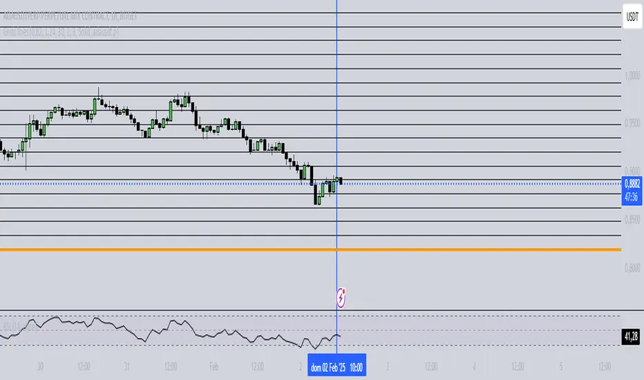
ICT Key Levels: PDH / PDL / Daily Open//@version=5
indicator("ICT Key Levels: PDH / PDL / Daily Open", shorttitle="ICT Levels", overlay=true)
// --- Inputs
showPD = input.bool(true, "Mostrar PDH/PDL")
showOpen = input.bool(true, "Mostrar Daily Open")
pdhColor = input.color(color.new(color.green, 0), "Color PDH")
pdlColor = input.color(color.new(color.red, 0), "Color PDL")
openColor = input.color(color.new(color.orange, 0), "Color Daily Open")
lineWidth = input.int(1, "Ancho líneas", minval=1, maxval=4)
// --- Previous day high / low (using daily security)
pdh = request.security(syminfo.tickerid, "D", high )
pdl = request.security(syminfo.tickerid, "D", low )
// --- Daily open (current day's open on Daily timeframe)
dailyOpen = request.security(syminfo.tickerid, "D", open)
// --- Plots
plot(showPD and not na(pdh) ? pdh : na, title="PDH", color=pdhColor, linewidth=lineWidth, style=plot.style_line)
plot(showPD and not na(pdl) ? pdl : na, title="PDL", color=pdlColor, linewidth=lineWidth, style=plot.style_line)
plot(showOpen and not na(dailyOpen) ? dailyOpen : na, title="Daily Open", color=openColor, linewidth=lineWidth, style=plot.style_line)
// --- Optional: etiquetas en inicio de día (solo en la primera barra diaria)
isNewDay = ta.change(time("D"))
labelNewDayOpen = input.bool(true, "Mostrar etiqueta en apertura diaria")
if labelNewDayOpen and isNewDay
label.new(bar_index, dailyOpen, text="Open", style=label.style_label_down, color=color.new(openColor,50), textcolor=color.black, yloc=yloc.price)

MOMO Exhaustion Short Signal Strategy v6 alexh1166Prints Short Signals for Exhausted Momentum stocks primed for reversals

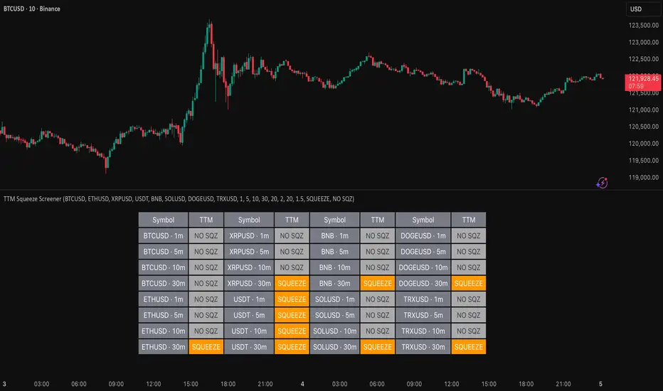
TTM Squeeze Screener [Pineify]TTM Squeeze Screener for Multiple Crypto Assets and Timeframes
This advanced TradingView Pine script, TTM Squeeze Screener, helps traders scan multiple crypto symbols and timeframes simultaneously, unlocking new dimensions in momentum and volatility analysis.
Key Features
Screen up to 8 crypto symbols across 4 different timeframes in one pane
TTM Squeeze indicator detects volatility contraction and expansion (“squeeze”) phases
Momentum filter reveals potential breakout direction and strength
Visual screener table for intuitive multi-asset monitoring
Fully customizable for symbols and timeframes
How It Works
The heart of this screener is the TTM Squeeze algorithm—a hybrid volatility and momentum indicator leveraging Bollinger Bands, Keltner Channels, and linear momentum analysis. The script checks whether Bollinger Bands are “squeezed” inside Keltner Channels, flagging periods of low volatility primed for expansion. Once a squeeze is released, the included momentum calculation suggests the likely breakout direction.
For each selected symbol and timeframe, the screener runs the TTM Squeeze logic, outputs “SQUEEZE” or “NO SQZ”, and tags momentum values. A table layout organizes the results, allowing rapid pattern recognition across symbols.
Trading Ideas and Insights
Spot multi-symbol volatility clusters—ideal for finding synchronized market moves
Assess breakout potential and direction before entering trades
Scalping and swing trading decisions are enhanced by cross-timeframe momentum filtering
Portfolio managers can quickly identify which assets are about to move
How Multiple Indicators Work Together
This screener unites three essential concepts:
Bollinger Bands : Measure volatility using standard deviation of price
Keltner Channels : Define expected price range based on average true range (ATR)
Momentum : Linear regression calculation to evaluate the direction and intensity after a squeeze
By combining these, the indicator not only signals when volatility compresses and releases, but also adds directional context—filtering false signals and helping traders time entries and exits more precisely.
Unique Aspects
Multi-symbol, multi-timeframe architecture—optimized for crypto traders and market scanners
Advanced table visualization—see all signals at a glance, minimizing cognitive overload
Modular calculation functions—easy to adapt and extend for other asset classes or strategies
Real-time, low-latency screening—built for actionable alerts on fast-moving markets
How to Use
Add the script to a TradingView chart (works on custom layouts)
Select up to 8 symbols and 4 timeframes using input fields (defaults to BTCUSD, ETHUSD, etc.)
Monitor the screener table; “SQUEEZE” highlights assets in potential breakout phase
Use momentum values to judge if the squeeze is likely bullish or bearish
Combine screener insights with manual chart analysis for optimal results
Customization
Symbols: Easily set any ticker for deep market scanning
Timeframes: Adjust to match your trading horizon (scalping, swing, long-term)
Indicator parameters: Refine Bollinger/Keltner/Momentum settings for sensitivity
Visuals: Personalize table layout, color codes, and formatting for clarity
Conclusion
In summary, the TTM Squeeze Screener is a robust, original TradingView indicator designed for crypto traders who demand a sophisticated multi-symbol, multi-timeframe edge. Its combination of volatility and momentum analytics makes it ideal for catching explosive breakouts, managing risk, and scanning the market efficiently. Whether you’re a scalper or swing trader, this screener provides the insights needed to stay ahead of the curve.
Mean Reversion Probability Zones [BigBeluga]🔵 OVERVIEW
The Mean Reversion Probability Zones indicator measures the likelihood of price reverting back toward its mean . By analyzing oscillator dynamics (RSI, MFI, or Stochastic), it calculates probability zones both above and below the oscillator. These zones are visualized as histograms, colored regions on the main chart, and a compact dashboard, helping traders spot when the market is statistically stretched and more likely to revert.
🔵 CONCEPTS
Mean Reversion : The tendency of price to return to its average after significant extensions.
Oscillator-Based Analysis : Uses RSI, MFI, or Stochastic as the base signal for detecting overextension.
Probability Model : The probability of reversion is computed using three factors:
Whether the oscillator is rising or declining.
Whether the oscillator is above or below user-defined thresholds.
The oscillator’s actual value (distance from equilibrium).
Dual-Zone Output :
Upper histogram = probability of downward mean reversion.
Lower histogram = probability of upward mean reversion.
Historical Extremes : The dashboard highlights the recent maximum probability values for both upward and downward scenarios.
🔵 FEATURES
Oscillator Choice : Switch between RSI, MFI, and Stochastic.
Customizable Zones : User-defined upper/lower thresholds with independent colors.
Probability Histograms :
Above oscillator → down reversion probability.
Below oscillator → up reversion probability.
Colored Gradient Zones on Chart : Visual overlays showing where mean reversion probabilities are strongest.
Probability Labels : Percentages displayed next to histogram values for clarity.
Dashboard : Compact table in the corner showing the recent maximum probabilities for both upward and downward mean reversion.
Overlay Compatibility : Works in both chart pane and sub-pane with oscillators.
🔵 HOW TO USE
Set Oscillator : Choose RSI, MFI, or Stochastic depending on your strategy style.
Adjust Zones : Define upper/lower bounds for when oscillator values indicate strong overbought/oversold conditions.
Interpret Histograms :
Orange (upper) histogram → higher chance of a pullback/downward mean reversion.
Green (lower) histogram → higher chance of upward reversion/bounce.
Watch Gradient Zones : On the main chart, shaded areas highlight where probability of mean reversion is elevated.
Consult Dashboard : Use the “Recent MAX” values to understand how strong recent reversion probabilities have been in either direction.
Confluence Strategy : Combine with support/resistance, order flow, or trend filters to avoid counter-trend trades.
🔵 CONCLUSION
The Mean Reversion Probability Zones provides traders with an advanced way to quantify and visualize mean reversion opportunities. By blending oscillator momentum, threshold logic, and probability calculations, it highlights when markets are statistically stretched and primed for reversal. Whether you are a contrarian trader or simply looking for exhaustion signals to fade, this tool helps bring structure and clarity to mean reversion setups.

BioSwarm Imprinter™BioSwarm Imprinter™ — Agent-Based Consensus for Traders
What it is
BioSwarm Imprinter™ is a non-repainting, agent-based sentiment oscillator. It fuses many short-to-medium lookback “opinions” into one 0–100 consensus line that is easy to read at a glance (50 = neutral, >55 bullish bias, <45 bearish bias). The engine borrows from swarm intelligence: many simple voters (agents) adapt their influence over time based on how well they’ve been predicting price, so the crowd gets smarter as conditions change.
Use it to:
• Detect emerging trends sooner without overreacting to noise.
• Filter mean-reversion vs continuation opportunities.
• Gate entries with a confidence score that reflects both strength and persistence of the move.
• Combine with your execution tools (VWAP/ORB/levels) as a state filter rather than a trade signal by itself.
⸻
Why it’s different
• Swarm learning: Each agent improves or decays its “fitness” depending on whether its vote matched the next bar’s direction. High-fitness agents matter more; weak agents fade.
• Multi-horizon by design: The crowd is composed of fixed, simple lookbacks spread from lenMin to lenMax. You get a blended, robust view instead of a single fragile parameter.
• Two complementary lenses: Each agent evaluates RSI-style balance (via Wilder’s RMA) and momentum (EMA deviation). You decide the weight of each.
• No repaint, no MTF pitfalls: Everything runs on the chart’s timeframe with bar-close confirmation; no request.security() or forward references.
• Actionable UI: A clean consensus line, optional regime background, confidence heat, and triangle markers when thresholds are crossed.
⸻
What you see on the chart
• Consensus line (0–100): Smoothed to your preference; color/area makes bull/bear zones obvious.
• Regime coloring (optional): Light green in bull zone, light red in bear zone; neutral otherwise.
• Confidence heat: A small gauge/number (0–100) that combines distance from neutral and recent persistence.
• Markers (optional): Triangles when consensus crosses up through your bull threshold (e.g., 55) or down through your bear threshold (e.g., 45).
• Info panel (optional): Consensus value, regime, confidence, number of agents, and basic diagnostics.
⸻
How it works (under the hood)
1. Horizon bins: The range is divided into numBins. Each bin has a fixed, simple integer length (crucial for Pine’s safety rules).
2. Per-bin features (computed every bar):
• RSI-style balance using Wilder’s RMA (not ta.rsi()), then mapped to −1…+1.
• Momentum as (close − EMA(L)) / EMA(L) (dimensionless drift).
3. Agent vote: For its assigned bin, an agent forms a weighted score: score = wRSI*RSI_like + wMOM*Momentum. A small dead-band near zero suppresses chop; votes are +1/−1/0.
4. Fitness update (bar close): If the agent’s previous vote agreed with the next bar’s direction, multiply its fitness by learnGain; otherwise by learnPain. Fitness is clamped so it never explodes or dies.
5. Consensus: Weighted average of all votes using fitness as weights → map to 0–100 and smooth with EMA.
Why it doesn’t repaint:
• No future references, no MTF resampling, fitness updates only on confirmed bars.
• All TA primitives (RMA/EMA/deltas) are computed every bar unconditionally.
⸻
Signals & confidence
• Bullish bias: consensus ≥ bullThr (e.g., 55).
• Bearish bias: consensus ≤ bearThr (e.g., 45).
• Confidence (0–100):
• Distance score: how far consensus is from 50.
• Momentum score: how strong the recent change is versus its recent average.
• Combined into a single gate; start filtering entries at ≥60 for higher quality.
Tip: For range sessions, raise thresholds (60/40) and increase smoothing; for momentum sessions, lower smoothing and keep thresholds at 55/45.
⸻
Inputs you’ll actually tune
• Agents & horizons:
• N_agents (e.g., 64–128)
• lenMin / lenMax (e.g., 6–30 intraday, 10–60 swing)
• numBins (e.g., 12–24)
• Weights & smoothing:
• wRSI vs wMOM (e.g., 0.7/0.3 for FX & indices; 0.6/0.4 for crypto)
• deadBand (0.03–0.08)
• consSmooth (3–8)
• Thresholds & hygiene:
• bullThr/bearThr (55/45 default)
• cooldownBars to avoid signal spam
⸻
Playbooks (ready-to-use)
1) Breakout / Trend continuation
• Timeframe: 15m–1h for day/swing.
• Filter: Take longs only when consensus > 55 and confidence ≥ 60.
• Execution: Use your ORB/VWAP/pullback trigger for entry. Trail with swing lows or 1.5×ATR. Exit on a close back under 50 or when a bearish signal prints.
2) Mean reversion (fade)
• When: Sideways days or low-volatility clusters.
• Setup: Increase deadBand and consSmooth.
• Signal: Bearish fades when consensus rolls over below ≈55 but stays above 50; bullish fades when it rolls up above ≈45 but stays below 50.
• Targets: The neutral zone (~50) as the first take-profit.
3) Multi-TF alignment
• Keep BioSwarm on 1H for bias, execute on 5–15m:
• Only take entries in the direction of the 1H consensus.
• Skip counter-bias scalps unless confidence is very low (explicit mean-reversion plan).
⸻
Integrations that work
• DynamoSent Pro+ (macro bias): Only act when macro bias and swarm consensus agree.
• ORB + Session VWAP Pro: Trade London/NY ORB breakouts that retest while consensus >55 (long) or <45 (short).
• Levels/Orderflow: BioSwarm is your “go / no-go”; execution stays with your usual triggers.
⸻
Quick start
1. Drop the indicator on a 1H chart.
2. Start with: N_agents=64, lenMin=6, lenMax=30, numBins=16, deadBand=0.06, consSmooth=5, thresholds 55/45.
3. Trade only when confidence ≥ 60.
4. Add your favorite execution tool (VWAP/levels/OR) for entries & exits.
⸻
Non-repainting & safety notes
• No request.security(); no hidden lookahead.
• Bar-close confirmation for fitness and signals.
• All TA calls are unconditional (no “sometimes called” warnings).
• No series-length inputs to RSI/EMA — we use RMA/EMA formulas that accept fixed simple ints per bin.
⸻
Known limits & tips
• Too many signals? Raise deadBand, increase consSmooth, widen thresholds to 60/40.
• Too few signals? Lower deadBand, reduce consSmooth, narrow thresholds to 53/47.
• Over-fitting risk: Keep learnGain/learnPain modest (e.g., ×1.04 / ×0.96).
• Compute load: Large N_agents × numBins is heavier; scale to your device.
⸻
Example recipes
EURUSD 1H (swing):
lenMin=8, lenMax=34, numBins=16, wRSI=0.7, wMOM=0.3, deadBand=0.06, consSmooth=6, thr=55/45
Buy breakouts when consensus >55 and confidence ≥60; confirm with 5–15m pullback to VWAP or level.
SPY 15m (US session):
lenMin=6, lenMax=24, numBins=12, consSmooth=4, deadBand=0.05
On trend days, stay with longs as long as consensus >55; add on shallow pullbacks.
BTC 1H (24/7):
Increase momentum weight: wRSI=0.6, wMOM=0.4, extend lenMax to ~50. Use dynamic stops (ATR) and partials on strong verticals.
⸻
Final word
BioSwarm is a state engine: it tells you when the market is primed to continue or mean-revert. Pair it with your entries and risk framework to turn that state into trades. If you’d like, I can supply a companion strategy template that consumes the consensus and back-tests the three playbooks (Breakout/Fade/Flip) with standard risk management.

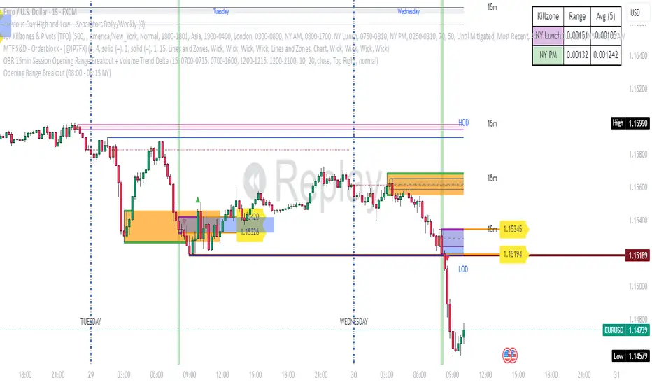
Opening Range Breakout (08:00 - 08:15 NY) - AAPNIndicador que marca la apertura de Forex en NY a 15 minitos, la primera vela
Momentum BandsMomentum Bands indicator-->technical tool that measures the rate of price change and surrounds this momentum with adaptive bands to highlight overbought and oversold zones. Unlike Bollinger Bands, which track price, these bands track momentum itself, offering a unique view of market strength and exhaustion points. At its core, it features a blue momentum line that calculates the rate of change over a set period, an upper red band marking dynamic resistance created by adding standard deviations to the momentum average, a lower green band marking dynamic support by subtracting standard deviations, and a gray middle line representing the average of momentum as a central anchor. When the momentum line touches or moves beyond the upper red band, it often signals that the market may be overbought and a pullback or reversal could follow; traders might lock in profits or watch for short setups. Conversely, when it drops below the lower green band, it can suggest an oversold market primed for a bounce, prompting traders to look for buying opportunities. If momentum remains between the bands, it typically indicates balanced conditions where waiting for stronger signals at the extremes is wise. The indicator can be used in contrarian strategies—buying near the lower band and selling near the upper—or in trend-following setups by waiting for momentum to return toward the centerline before entering trades. For stronger confirmation, traders often combine it with volume spikes, support and resistance analysis, or other trend tools, and it’s useful to check multiple timeframes to spot consistent patterns. Recommended settings vary: short-term traders might use a 7–10 period momentum with 14-period bands; medium-term traders might keep the default 14-period momentum and 20-period bands; while long-term analysis might use 21-period momentum and 50-period bands. Visually, background colors help spot extremes: red for strong overbought, green for strong oversold, and no color for normal markets, alongside reference lines at 70, 30, and 0 to guide traditional overbought, oversold, and neutral zones. Typical bullish signals include momentum rebounding from the lower band, crossing back above the middle after being oversold, or showing divergence where price makes new lows but momentum doesn’t. Bearish signals might appear when momentum hits the upper band and weakens, drops below the middle after being overbought, or price makes new highs while momentum fails to follow. The indicator tends to work best in mean-reverting or sideways markets rather than strong trends, where overbought and oversold conditions tend to repeat.
MACD+RSI Indicator Moving Average Convergence/Divergence or MACD is a momentum indicator that shows the relationship between two Exponential Moving Averages (EMAs) of a stock price. Convergence happens when two moving averages move toward one another, while divergence occurs when the moving averages move away from each other. This indicator also helps traders to know whether the stock is being extensively bought or sold. Its ability to identify and assess short-term price movements makes this indicator quite useful.
The Moving Average Convergence/Divergence indicator was invented by Gerald Appel in 1979.
Moving Average Convergence/Divergence is calculated using a 12-day EMA and 26-day EMA. It is important to note that both the EMAs are based on closing prices. The convergence and divergence (CD) values have to be calculated first. The CD value is calculated by subtracting the 26-day EMA from the 12-day EMA.
---------------------------------------------------------------------------------------------------------------------
The relative strength index (RSI) is a momentum indicator used in technical analysis. RSI measures the speed and magnitude of a security's recent price changes to detect overbought or oversold conditions in the price of that security.
The RSI is displayed as an oscillator (a line graph) on a scale of zero to 100. The indicator was developed by J. Welles Wilder Jr. and introduced in his seminal 1978 book, New Concepts in Technical Trading Systems.
In addition to identifying overbought and oversold securities, the RSI can also indicate securities that may be primed for a trend reversal or a corrective pullback in price. It can signal when to buy and sell. Traditionally, an RSI reading of 70 or above indicates an overbought condition. A reading of 30 or below indicates an oversold condition.
---------------------------------------------------------------------------------------------------------------------
By combining them, you can create a MACD/RSI strategy. You can go ahead and search for MACD/RSI strategy on any social platform. It is so powerful that it is the most used indicator in TradingView. It is best for trending market. Our indicator literally let you customize MACD/RSI settings. Explore our indicator by applying to your chart and start trading now!

Bradley SiderographThis indicator functions as a Planetary Barometer, bringing the Bradley-Siderograph directly onto your TradingView chart. Designed for tracking the algebraic sum of planetary aspects and declination values in relation to market movements, it analyzes sidereal potential, long-term and mid-term planetary aspects, and the declination factor to provide insight into potential shifts in mass psychology. The built-in gauges act like a barometer, visually measuring the intensity and range of the components.
As Donald Bradley states in Stock Market Prediction:
" The siderograph is nothing more than a time chart showing a wavy line, which represents the algebraic total of the declination factor, the long terms, and the middle terms. It can be computed for any period—past or future—for which an ephemeris is available. Every aspect, whether long or middle term, is assigned a theoretical value of 10 at its peak. The value of the declination factor is half the algebraic sum of the given declinations of Venus and Mars, with northern declination considered positive and southern declination negative. "
How the Bradley-Siderograph Works:
The Siderograph assigns positive and negative valencies based on the transits of inner and outer planets, categorized into long-term and mid-term aspects.
Each aspect (15° orb) is given a theoretical value, with the peak set at ±10. The approach and separation phases influence the weighting of each aspect leading up to its peak.
The sign of the valency depends on the type of aspect:
Squares and oppositions are assigned negative values
Trines and sextiles are assigned positive values
Conjunctions can be either positive or negative, depending on the planetary combination
Formula Used:
The Siderograph is computed as follows:
𝑃 = 𝑋 (𝐿 + 𝐷) + 𝑀
Where:
P = Sidereal Potential (final computed value)
X = Multiplier (to weight long-term aspects)
L = Long-term aspects (10 aspect combinations)
D = Declination factor (half the sum of Venus and Mars declinations)
M = Mid-term aspects
The long-term component (L + D) can be multiplied by a chosen factor (X) to emphasize its influence relative to the mid-term aspects.
How to Use the Indicator:
Once applied, the Siderograph line overlays on the chart, using the left-side scale for reference.
The indicator provides separate plots for:
Sidereal potential
Long-term aspects
Mid-term aspects
Declination factor
Each component can be toggled on or off for deeper analysis.
Gauges "provided by @faiyaz7283 library" display the high and low range for each curve, allowing quick identification of extreme values.
The indicator also marks the yearly high and low of the current year’s sidereal potential, providing a reference for when the market is trading above or below key levels. This feature was inspired by an observation made by Bradley in his book, which I wanted to incorporate here.
Users can fully customize the indicator by:
Switching between geocentric and heliocentric views.
Adjusting the orb of planetary transits to refine aspect sensitivity.
Multiplier (to weight long-term aspects)
Explore the Bradley-Siderograph and experiment with its settings.
Main Use Case
The Siderograph can be thought of as a psychological wind sock, gauging shifts in mass sentiment in response to planetary influences. Rather than forecasting market direction outright, it serves as an early warning system, signaling when conditions may be primed for changes in collective psychology.
As Donald Bradley notes in Stock Market Prediction:
" A limitation of the siderograph is that it cannot be construed as a forecast of secular trend. In statistical terminology, 'lines of regression' fitted to the market course and to the potential should not be expected to completely agree, for reasons obvious to everybody with keen business sense or commercial training. However, the siderograph may be depended upon to reward its analyst with foreknowledge of coming conditions in general, so that the non-psychological factors may be evaluated accordingly. By this, we mean that the potential will afford one with clues as to how the mass mind will 'take' the other mechanical or governmental vicissitudes affecting high finance. The siderograph may be thought of as a principle 'symptom' in diagnosing current market circumstances and as a sounding-board for prognoses concerning further developments. "
Planned Improvement:
While Bradley did not construct the Siderograph for direct forecasting, an enhancement to this indicator would be the ability to project each curve forward in time, providing a clearer view of how upcoming planetary aspects.
This indicator is being released as open source with the hope of further refining and expanding its capabilities—particularly in developing future plots that improve visualization and analysis. Contributions and feedback are encouraged to enhance its usability and advance the study of planetary influences in market behavior.
Credits & Acknowledgments:
Inspired by Donald Bradley and his work in Stock Market Prediction: The Planetary Barometer and How to Use It.
Built using Astrolib, developed by @BarefootJoey
Built using Gauges, developed by @faiyaz7283

Grids lines"Líneas de Grid para Análisis Técnico"
Este indicador dibuja líneas de grid (rejilla) en el gráfico de precios, lo que puede ayudar a visualizar zonas de soporte, resistencia y niveles de interés en un rango de precios determinado.
Características:
Precio Mínimo y Máximo: Configura los precios entre los cuales se dibujarán las líneas de grid.
Número de Grids: Establece cuántas líneas de grid quieres ver en el gráfico.
Color y Grosor de las Líneas: Personaliza los colores y el grosor de las líneas de grid, incluyendo la primera y la última línea.
Estilo de las Líneas: Puedes elegir entre líneas discontinuas (Dotted) o sólidas (Solid), para personalizar aún más tu visualización.
Ticker Específico: Si lo deseas, puedes elegir un ticker específico para dibujar las líneas solo cuando el gráfico esté mostrando ese activo. De lo contrario, las líneas se dibujarán en el gráfico actual.
Parámetros:
Precio Mínimo: El precio más bajo para el rango del grid (por ejemplo: 0.82).
Precio Máximo: El precio más alto para el rango del grid (por ejemplo: 1.24).
Número de Grids: Define cuántas líneas quieres entre el precio mínimo y el máximo (por ejemplo: 30).
Estilo de Línea: Elige entre Dotted (líneas discontinuas) o Solid (líneas sólidas).
Ticker: Si deseas dibujar las líneas solo para un ticker específico, ingresa el símbolo del ticker (por ejemplo, ADAUSDT). Si dejas este campo vacío, las líneas se dibujarán en el gráfico actual.
Ejemplo de Uso:
Si estás analizando el par ADAUSDT, puedes escribir ADAUSDT en el campo del ticker para que las líneas solo se dibujen cuando este par esté visible. Si dejas el campo vacío, las líneas se dibujarán en cualquier ticker que tengas en el gráfico.
Descripción en Inglés:
"Grid Lines for Technical Analysis"
This indicator draws grid lines on the price chart, helping to visualize support, resistance, and key levels within a specific price range.
Features:
Min and Max Price: Set the price range for the grid lines to be drawn.
Number of Grids: Choose how many grid lines you want to display on the chart.
Line Color and Thickness: Customize the color and thickness of the grid lines, including the first and last line.
Line Style: Choose between Dotted (dashed lines) or Solid (solid lines) to further customize your view.
Specific Ticker: If desired, you can specify a ticker for the grid lines to only be drawn when that asset is shown. Otherwise, the lines will be drawn on the current chart.
Parameters:
Min Price: The lowest price for the grid range (for example, 0.82).
Max Price: The highest price for the grid range (for example, 1.24).
Number of Grids: Defines how many lines you want between the minimum and maximum price (for example, 30).
Line Style: Choose between Dotted or Solid.
Ticker: To draw the lines only for a specific ticker, enter the symbol of the ticker (for example, ADAUSDT). If left blank, the lines will be drawn on the current ticker.
Usage Example:
If you're analyzing the pair ADAUSDT, you can enter ADAUSDT in the ticker field to draw the lines only when that pair is visible. If you leave the field blank, the lines will be drawn for any ticker currently on the chart.
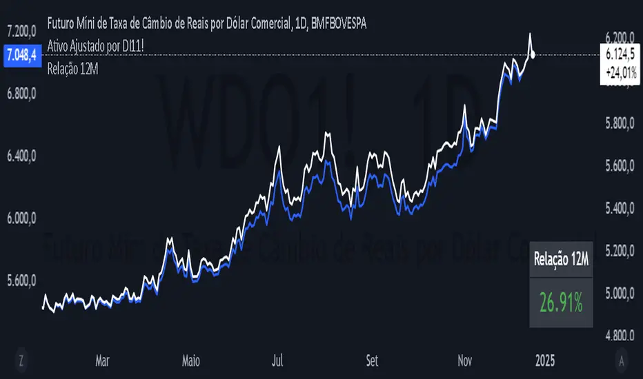
12 Month Difference - YoY ComparisonEste script foi desenvolvido para calcular e exibir a variação percentual do preço de um ativo nos últimos 12 meses, de forma simples e visual. Ele utiliza dados históricos de preços e apresenta o resultado diretamente no gráfico, permitindo ao usuário acompanhar a relação entre o valor atual e o valor de 12 meses atrás.
O cálculo é baseado em um período de 12 meses, que equivale a 252 dias úteis no mercado financeiro. O script primeiro identifica o preço atual do ativo e o compara com o preço registrado há exatamente 252 dias úteis. A diferença entre esses dois valores é transformada em uma variação percentual, o que facilita a análise de desempenho do ativo ao longo do período.
Além disso, o script define uma cor para destacar o resultado:
Verde, se a variação percentual for positiva (indicando crescimento).
Vermelho, se a variação for negativa (indicando queda).
O valor calculado é exibido de forma prática no canto inferior direito do gráfico, como uma tabela flutuante. Essa tabela contém o texto "Relação 12M" e o valor percentual correspondente, permitindo uma leitura rápida.
Embora o resultado seja calculado para todos os momentos no gráfico, ele é mostrado apenas como uma tabela no último ponto confirmado da série histórica, ou seja, no momento mais recente com dados disponíveis. Além disso, o script inclui o valor da relação na legenda do gráfico, mas ele está oculto visualmente para evitar sobrecarregar o layout.
Esse indicador é útil para analisar rapidamente o desempenho de um ativo ao longo de um ano, ajudando investidores e analistas a entenderem tendências e mudanças no mercado.
This script was developed to calculate and display the percentage change in the price of an asset over the last 12 months, in a simple and visual way. It uses historical price data and displays the result directly on the chart, allowing the user to monitor the relationship between the current value and the value from 12 months ago.
The calculation is based on a 12-month period, which is equivalent to 252 business days in the financial market. The script first identifies the current price of the asset and compares it with the price recorded exactly 252 business days ago. The difference between these two values is transformed into a percentage change, which makes it easier to analyze the asset's performance over the period.
In addition, the script defines a color to highlight the result:
Green, if the percentage change is positive (indicating growth).
Red, if the change is negative (indicating a decline).
The calculated value is displayed conveniently in the bottom right corner of the chart, as a floating table. This table contains the text "12M Ratio" and the corresponding percentage value, allowing for quick reading.
Although the result is calculated for all points in time on the chart, it is only displayed as a table at the last confirmed point in the historical series, i.e. the most recent point in time with available data. In addition, the script includes the ratio value in the chart legend, but it is visually hidden to avoid cluttering the layout.
This indicator is useful for quickly analyzing the performance of an asset over a year, helping investors and analysts understand trends and changes in the market.
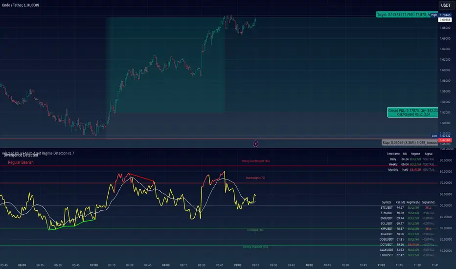
Adapted RSI w/ Multi-Asset Regime Detection v1.1The relative strength index (RSI) is a momentum indicator used in technical analysis. RSI measures the speed and magnitude of an asset's recent price changes to detect overbought or oversold conditions in the price of said asset.
In addition to identifying overbought and oversold assets, the RSI can also indicate whether your desired asset may be primed for a trend reversal or a corrective pullback in price. It can signal when to buy and sell.
The RSI will oscillate between 0 and 100. Traditionally, an RSI reading of 70 or above indicates an overbought condition. A reading of 30 or below indicates an oversold condition.
The RSI is one of the most popular technical indicators. I intend to offer a fresh spin.
Adapted RSI w/ Multi-Asset Regime Detection
Our Adapted RSI makes necessary improvements to the original Relative Strength Index (RSI) by combining multi-timeframe analysis with multi-asset monitoring and providing traders with an efficient way to analyse market-wide conditions across different timeframes and assets simultaneously. The indicator automatically detects market regimes and generates clear signals based on RSI levels, presenting this data in an organised, easy-to-read format through two dynamic tables. Simplicity is key, and having access to more RSI data at any given time, allows traders to prepare more effectively, especially when trading markets that "move" together.
How we calculate the RSI
First, the RSI identifies price changes between periods, calculating gains and losses from one look-back period to the next. This look-back period averages gains and losses over 14 periods, which in this case would be 14 days, and those gains/losses are calculated based on the daily closing price. For example:
Average Gain = Sum of Gains over the past 14 days / 14
Average Loss = Sum of Losses over the past 14 days / 14
Then we calculate the Relative Strength (RS):
RS = Average Gain / Average Loss
Finally, this is converted to the RSI value:
RSI = 100 - (100 / (1 + RS))
Key Features
Our multi-timeframe RSI indicator enhances traditional technical analysis by offering synchronised Daily, Weekly, and Monthly RSI readings with automatic regime detection. The multi-asset monitoring system allows tracking of up to 10 different assets simultaneously, with pre-configured major pairs that can be customised to any asset selection. The signal generation system provides clear market guidance through automatic regime detection and a five-level signal system, all presented through a sophisticated visual interface with dynamic RSI line colouring and customisable display options.
Quick Guide to Use it
Begin by adding the indicator to your chart and configuring your preferred assets in the "Asset Comparison" settings.
Position the two information tables according to your preference.
The main table displays RSI analysis across three timeframes for your current asset, while the asset table shows a comparative analysis of all monitored assets.
Signals are colour-coded for instant recognition, with green indicating bullish conditions and red for bearish conditions. Pay special attention to regime changes and signal transitions, using multi-timeframe confluence to identify stronger signals.
How it Works (Regime Detection & Signals)
When we say 'Regime', a regime is determined by a persistent trend or in this case momentum and by leveraging this for RSI, which is a momentum oscillator, our indicator employs a relatively simple regime detection system that classifies market conditions as either Bullish (RSI > 50) or Bearish (RSI < 50). Our benchmark between a trending bullish or bearish market is equal to 50. By leveraging a simple classification system helps determine the probability of trend continuation and the weight given to various signals. Whilst we could determine a Neutral regime for consolidating markets, we have employed a 'neutral' signal generation which will be further discussed below...
Signal generation occurs across five distinct levels:
Strong Buy (RSI < 15)
Buy (RSI < 30)
Neutral (RSI 30-70)
Sell (RSI > 70)
Strong Sell (RSI > 85)
Each level represents different market conditions and probability scenarios. For instance, extreme readings (Strong Buy/Sell) indicate the highest probability of mean reversion, while neutral readings suggest equilibrium conditions where traders should focus on the overall regime bias (Bullish/Bearish momentum).
This approach offers traders a new and fresh spin on a popular and well-known tool in technical analysis, allowing traders to make better and more informed decisions from the well presented information across multiple assets and timeframes. Experienced and beginner traders alike, I hope you enjoy this adaptation.
RSItrendsThis is to my friends and to my sons to use.
What Is the Relative Strength Index (RSI)?
The relative strength index (RSI) is a momentum indicator used in technical analysis. RSI measures the speed and magnitude of a security's recent price changes to evaluate overvalued or undervalued conditions in the price of that security.
The RSI is displayed as an oscillator (a line graph) on a scale of zero to 100. The indicator was developed by J. Welles Wilder Jr. and introduced in his seminal 1978 book, New Concepts in Technical Trading Systems.
1
The RSI can do more than point to overbought and oversold securities. It can also indicate securities that may be primed for a trend reversal or corrective pullback in price. It can signal when to buy and sell. Traditionally, an RSI reading of 70 or above indicates an overbought situation. A reading of 30 or below indicates an oversold condition.