Adjustable Vertical LinesThe script provides an indicator which will plot lines - 15 min, 30 min and 60 min. You can customize the time intervals and go to as low as one minute, but I found the 15-minute and 30-minute intervals works best for me when trying to find setups, and the lower time-frame intervals, is just pointless to use if you're not scalping on the seconds timeframe.
You can customize inputs for the line style. Line thickness, colour, etc.
I've seen this work using the OBR theory and applying it to the one-minute candle then looking for other confluences like order blocks, or breakers, FVGs, BOS/CHoC for further confirmation for scalping. It's important to backtest though and see for yourself.
Thanks for the boost.
Pesquisar nos scripts por "机械革命无界15+时不时闪屏"

Momentum Fusion v1Momentum Fusion v1
Overview
Momentum Fusion v1 (MFusion) is a multi-oscillator indicator that combines several components to analyze market momentum and trend strength. It incorporates modified versions of classic indicators such as PVI (Positive Volume Index), NVI (Negative Volume Index), MFI (Money Flow Index), RSI, Stochastic, and Bollinger Bands Oscillator. The indicator displays a histogram that changes color based on momentum strength and includes "FUSION🔥" signal labels when extreme values are reached.
Indicator Settings
Parameters:
EMA Length – Smoothing period for the moving average (default: 255).
Smoothing Period – Internal calculation smoothing parameter (default: 15).
BB Multiplier – Standard deviation multiplier for Bollinger Bands (default: 2.0).
Show verde / marron / media lines – Toggles the display of auxiliary lines.
Show FUSION🔥 label – Enables/disables signal labels.
Indicator Components
1. PVI (Positive Volume Index)
Formula:
pvi := volume > volume ? nz(pvi ) + (close - close ) / close * sval : nz(pvi )
Description:
PVI increases when volume rises compared to the previous bar and accounts for price percentage change. The stronger the price movement with increasing volume, the higher the PVI value.
2. NVI (Negative Volume Index)
Formula:
nvi := volume < volume ? nz(nvi ) + (close - close ) / close * sval : nz(nvi )
Description:
NVI tracks price movements during declining volume. If the price rises on low volume, it may indicate a "stealth" trend.
3. Money Flow Index (MFI)
Formula:
100 - 100 / (1 + up / dn)
Description:
An oscillator measuring money flow strength. Values above 80 suggest overbought conditions, while values below 20 indicate oversold conditions.
4. Stochastic Oscillator
Formula:
k = 100 * (close - lowest(low, length)) / (highest(high, length) - lowest(low, length))
Description:
A classic stochastic oscillator showing price position relative to the selected period's range.
5. Bollinger Bands Oscillator
Formula:
(tprice - BB midline) / (upper BB - lower BB) * 100
Description:
Indicates the price position relative to Bollinger Bands in percentage terms.
Key Lines & Histogram
1. Verde (Green Line)
Calculation:
verde = marron + oscp (normalized PVI)
Interpretation:
Higher values indicate stronger bullish momentum. A FUSION🔥 signal appears when the value reaches 750+.
2. Marron (Brown Line)
Calculation:
marron = (RSI + MFI + Bollinger Osc + Stochastic / 3) / 2
Interpretation:
A composite oscillator combining multiple indicators. Higher values suggest overbought conditions.
3. Media (Red Line)
Calculation:
media = EMA of marron with smoothing period
Interpretation:
Acts as a signal line for trend confirmation.
4. Histogram
Calculation:
histo = verde - marron
Colors:
Bright green (>100) – Strong bullish momentum.
Light green (>0) – Moderate bullish momentum.
Orange (<0) – Bearish momentum.
Red (<-100) – Strong bearish momentum.
Signals & Alerts
1. FUSION🔥 (Strong Momentum)
Condition:
verde >= 750
Visualization:
A "FUSION🔥" label appears below the chart.
Alert:
Can be set to trigger notifications when the condition is met.
2. Background Aura
Condition:
verde > 850
Visualization:
The chart background turns teal, indicating extreme momentum.
Usage Recommendations
FUSION🔥 Signal – Can be used as a long entry point when confirmed by other indicators.
Histogram:
1. Green bars – Potential long entry.
2. Red/orange bars – Potential short entry.
3. Media & Marron Crossover – Can serve as an additional trend filter.
4. Suitable for a 5-15 minute time frame
Conclusion
Momentum Fusion v1 is a powerful tool for momentum analysis, combining multiple indicators into a unified system. It is suitable for:
Trend traders (catching strong movements).
Scalpers (identifying short-term impulses).
Swing traders (filtering entry points).
The indicator features customizable settings and visual signals, making it adaptable to various trading styles.

MirPapa_Library_ICTLibrary "MirPapa_Library_ICT"
GetHTFoffsetToLTFoffset(_offset, _chartTf, _htfTf)
GetHTFoffsetToLTFoffset
@description Adjust an HTF offset to an LTF offset by calculating the ratio of timeframes.
Parameters:
_offset (int) : int The HTF bar offset (0 means current HTF bar).
_chartTf (string) : string The current chart’s timeframe (e.g., "5", "15", "1D").
_htfTf (string) : string The High Time Frame string (e.g., "60", "1D").
@return int The corresponding LTF bar index. Returns 0 if the result is negative.
IsConditionState(_type, _isBull, _level, _open, _close, _open1, _close1, _low1, _low2, _low3, _low4, _high1, _high2, _high3, _high4)
IsConditionState
@description Evaluate a condition state based on type for COB, FVG, or FOB.
Overloaded: first signature handles COB, second handles FVG/FOB.
Parameters:
_type (string) : string Condition type ("cob", "fvg", "fob").
_isBull (bool) : bool Direction flag: true for bullish, false for bearish.
_level (int) : int Swing level (only used for COB).
_open (float) : float Current bar open price (only for COB).
_close (float) : float Current bar close price (only for COB).
_open1 (float) : float Previous bar open price (only for COB).
_close1 (float) : float Previous bar close price (only for COB).
_low1 (float) : float Low 1 bar ago (only for COB).
_low2 (float) : float Low 2 bars ago (only for COB).
_low3 (float) : float Low 3 bars ago (only for COB).
_low4 (float) : float Low 4 bars ago (only for COB).
_high1 (float) : float High 1 bar ago (only for COB).
_high2 (float) : float High 2 bars ago (only for COB).
_high3 (float) : float High 3 bars ago (only for COB).
_high4 (float) : float High 4 bars ago (only for COB).
@return bool True if the specified condition is met, false otherwise.
IsConditionState(_type, _isBull, _pricePrev, _priceNow)
IsConditionState
@description Evaluate FVG or FOB condition based on price movement.
Parameters:
_type (string) : string Condition type ("fvg", "fob").
_isBull (bool) : bool Direction flag: true for bullish, false for bearish.
_pricePrev (float) : float Previous price (for FVG/FOB).
_priceNow (float) : float Current price (for FVG/FOB).
@return bool True if the specified condition is met, false otherwise.
IsSwingHighLow(_isBull, _level, _open, _close, _open1, _close1, _low1, _low2, _low3, _low4, _high1, _high2, _high3, _high4)
IsSwingHighLow
@description Public wrapper for isSwingHighLow.
Parameters:
_isBull (bool) : bool Direction flag: true for bullish, false for bearish.
_level (int) : int Swing level (1 or 2).
_open (float) : float Current bar open price.
_close (float) : float Current bar close price.
_open1 (float) : float Previous bar open price.
_close1 (float) : float Previous bar close price.
_low1 (float) : float Low 1 bar ago.
_low2 (float) : float Low 2 bars ago.
_low3 (float) : float Low 3 bars ago.
_low4 (float) : float Low 4 bars ago.
_high1 (float) : float High 1 bar ago.
_high2 (float) : float High 2 bars ago.
_high3 (float) : float High 3 bars ago.
_high4 (float) : float High 4 bars ago.
@return bool True if swing condition is met, false otherwise.
AddBox(_left, _right, _top, _bot, _xloc, _colorBG, _colorBD)
AddBox
@description Draw a rectangular box on the chart with specified coordinates and colors.
Parameters:
_left (int) : int Left bar index for the box.
_right (int) : int Right bar index for the box.
_top (float) : float Top price coordinate for the box.
_bot (float) : float Bottom price coordinate for the box.
_xloc (string) : string X-axis location type (e.g., xloc.bar_index).
_colorBG (color) : color Background color for the box.
_colorBD (color) : color Border color for the box.
@return box Returns the created box object.
Addline(_x, _y, _xloc, _color, _width)
Addline
@description Draw a vertical or horizontal line at specified coordinates.
Parameters:
_x (int) : int X-coordinate for start (bar index).
_y (int) : float Y-coordinate for start (price).
_xloc (string) : string X-axis location type (e.g., xloc.bar_index).
_color (color) : color Line color.
_width (int) : int Line width.
@return line Returns the created line object.
Addline(_x, _y, _xloc, _color, _width)
Parameters:
_x (int)
_y (float)
_xloc (string)
_color (color)
_width (int)
Addline(_x1, _y1, _x2, _y2, _xloc, _color, _width)
Parameters:
_x1 (int)
_y1 (int)
_x2 (int)
_y2 (int)
_xloc (string)
_color (color)
_width (int)
Addline(_x1, _y1, _x2, _y2, _xloc, _color, _width)
Parameters:
_x1 (int)
_y1 (int)
_x2 (int)
_y2 (float)
_xloc (string)
_color (color)
_width (int)
Addline(_x1, _y1, _x2, _y2, _xloc, _color, _width)
Parameters:
_x1 (int)
_y1 (float)
_x2 (int)
_y2 (int)
_xloc (string)
_color (color)
_width (int)
Addline(_x1, _y1, _x2, _y2, _xloc, _color, _width)
Parameters:
_x1 (int)
_y1 (float)
_x2 (int)
_y2 (float)
_xloc (string)
_color (color)
_width (int)
AddlineMid(_type, _left, _right, _top, _bot, _xloc, _color, _width)
AddlineMid
@description Draw a midline between top and bottom for FVG or FOB types.
Parameters:
_type (string) : string Type identifier: "fvg" or "fob".
_left (int) : int Left bar index for midline start.
_right (int) : int Right bar index for midline end.
_top (float) : float Top price of the region.
_bot (float) : float Bottom price of the region.
_xloc (string) : string X-axis location type (e.g., xloc.bar_index).
_color (color) : color Line color.
_width (int) : int Line width.
@return line or na Returns the created line or na if type is not recognized.
GetHtfFromLabel(_label)
GetHtfFromLabel
@description Convert a Korean HTF label into a Pine Script timeframe string via handler library.
Parameters:
_label (string) : string The Korean label (e.g., "5분", "1시간").
@return string Returns the corresponding Pine Script timeframe (e.g., "5", "60").
IsChartTFcomparisonHTF(_chartTf, _htfTf)
IsChartTFcomparisonHTF
@description Determine whether a given HTF is greater than or equal to the current chart timeframe.
Parameters:
_chartTf (string) : string Current chart timeframe (e.g., "5", "15", "1D").
_htfTf (string) : string HTF timeframe (e.g., "60", "1D").
@return bool True if HTF ≥ chartTF, false otherwise.
CreateBoxData(_type, _isBull, _useLine, _top, _bot, _xloc, _colorBG, _colorBD, _offset, _htfTf, htfBarIdx, _basePoint)
CreateBoxData
@description Create and draw a box and optional midline for given type and parameters. Returns success flag and BoxData.
Parameters:
_type (string) : string Type identifier: "fvg", "fob", "cob", or "sweep".
_isBull (bool) : bool Direction flag: true for bullish, false for bearish.
_useLine (bool) : bool Whether to draw a midline inside the box.
_top (float) : float Top price of the box region.
_bot (float) : float Bottom price of the box region.
_xloc (string) : string X-axis location type (e.g., xloc.bar_index).
_colorBG (color) : color Background color for the box.
_colorBD (color) : color Border color for the box.
_offset (int) : int HTF bar offset (0 means current HTF bar).
_htfTf (string) : string HTF timeframe string (e.g., "60", "1D").
htfBarIdx (int) : int HTF bar_index (passed from HTF request).
_basePoint (float) : float Base point for breakout checks.
@return tuple(bool, BoxData) Returns a boolean indicating success and the created BoxData struct.
ProcessBoxDatas(_datas, _useMidLine, _closeCount, _colorClose)
ProcessBoxDatas
@description Process an array of BoxData structs: extend, record volume, update stage, and finalize boxes.
Parameters:
_datas (array) : array Array of BoxData objects to process.
_useMidLine (bool) : bool Whether to update the midline endpoint.
_closeCount (int) : int Number of touches required to close the box.
_colorClose (color) : color Color to apply when a box closes.
@return void No return value; updates are in-place.
BoxData
Fields:
_isActive (series bool)
_isBull (series bool)
_box (series box)
_line (series line)
_basePoint (series float)
_boxTop (series float)
_boxBot (series float)
_stage (series int)
_isStay (series bool)
_volBuy (series float)
_volSell (series float)
_result (series string)
LineData
Fields:
_isActive (series bool)
_isBull (series bool)
_line (series line)
_basePoint (series float)
_stage (series int)
_isStay (series bool)
_result (series string)

MirPapa_Handler_HTFLibrary "MirPapa_Handler_HTF"
High Time Frame Handler Library:
Provides utilities for working with High Time Frame (HTF) and chart (LTF) conversions and data retrieval.
IsChartTFcomparisonHTF(_chartTf, _htfTf)
IsChartTFcomparisonHTF
@description
Determine whether the given High Time Frame (HTF) is greater than or equal to the current chart timeframe.
Parameters:
_chartTf (string) : The current chart’s timeframe string (examples: "5", "15", "1D").
_htfTf (string) : The High Time Frame string to compare (examples: "60", "1D").
@return
Returns true if HTF minutes ≥ chart minutes, false otherwise or na if conversion fails.
GetHTFrevised(_tf, _case)
GetHTFrevised
@description
Retrieve a specific bar value from a Higher Time Frame (HTF) series.
Supports current and historical OHLC values, based on a case identifier.
Parameters:
_tf (string) : The target HTF string (examples: "60", "1D").
_case (string) : A case string determining which OHLC value and bar offset to request:
"b" → HTF bar_index
"o" → HTF open
"h" → HTF high
"l" → HTF low
"c" → HTF close
"o1" → HTF open one bar ago
"h1" → HTF high one bar ago
"l1" → HTF low one bar ago
"c1" → HTF close one bar ago
… up to "o5", "h5", "l5", "c5" for five bars ago.
@return
Returns the requested HTF value or na if _case does not match any condition.
GetHTFfromLabel(_label)
GetHTFfromLabel
@description
Convert a Korean HTF label into a Pine Script-recognizable timeframe string.
Examples:
"5분" → "5"
"1시간" → "60"
"일봉" → "1D"
"주봉" → "1W"
"월봉" → "1M"
"연봉" → "12M"
Parameters:
_label (string) : The Korean HTF label string (examples: "5분", "1시간", "일봉").
@return
Returns the Pine Script timeframe string corresponding to the label, or "1W" if no match is found.
GetHTFoffsetToLTFoffset(_offset, _chartTf, _htfTf)
GetHTFoffsetToLTFoffset
@description
Adjust an HTF bar index and offset so that it aligns with the current chart’s bar index.
Useful for retrieving historical HTF data on an LTF chart.
Parameters:
_offset (int) : The HTF bar offset (0 means current HTF bar, 1 means one bar ago, etc.).
_chartTf (string) : The current chart’s timeframe string (examples: "5", "15", "1D").
_htfTf (string) : The High Time Frame string to align (examples: "60", "1D").
@return
Returns the corresponding LTF bar index after applying HTF offset. If result is negative, returns 0.
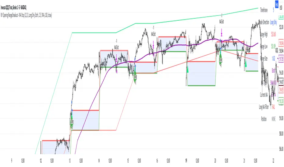
NY Opening Range Breakout - MA StopCore Concept
This strategy trades breakouts from the New York opening range (9:30-9:45 AM NY time) on intraday timeframes, designed for scalping and day trading.
Setup Requirements
Timeframe: Works on any timeframe under 15 minutes (1m, 2m, 3m, 5m, 10m)
Session: New York market hours
Range Period: 9:30-9:45 AM NY time (15-minute opening range)
Entry Rules
Long Entries:
Wait for a candle to close above the opening range high
Enter long on the next candle (before 12:00 PM NY time)
Must be above moving average if using MA-based take profit
Short Entries:
Wait for a candle to close below the opening range low
Enter short on the next candle (before 12:00 PM NY time)
Must be below moving average if using MA-based take profit
Risk Management
Stop Loss:
Long trades: Opening range low
Short trades: Opening range high
Take Profit Options:
Fixed Risk Reward: 1.5x the range size (customizable ratio)
Moving Average: Exit when price crosses back through MA
Both: Whichever comes first
Key Features
Trade Direction Options:
Long Only
Short Only
Both directions
Moving Average Filter:
Prevents entries that would immediately hit stop loss
Uses EMA/SMA/WMA/VWMA with customizable length
Acts as dynamic support/resistance
Time Restrictions:
No entries after 12:00 PM NY time (customizable cutoff)
One trade per direction per day
Daily reset of all variables
Visual Elements
Red/green lines showing opening range
Purple line for moving average
Entry and breakout signals with shapes
Take profit and stop loss levels plotted
Information table with current status
Strategy Logic Flow
Morning: Capture 9:30-9:45 range high/low
Wait: Monitor for breakout (previous candle close outside range)
Filter: Check MA condition if using MA-based exits
Enter: Trade on next candle after breakout
Manage: Exit at fixed TP, MA cross, or stop loss
Reset: Start fresh next trading day
This is a momentum-based breakout strategy that capitalizes on early market volatility while using the opening range as natural support/resistance levels.
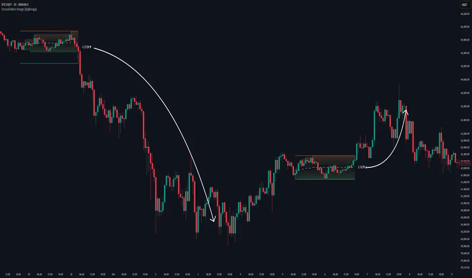
Consolidation Range [BigBeluga]A hybrid volatility-volume indicator that isolates periods of price equilibrium and reveals the directional force behind each range buildup.
Consolidation Range is a powerful tool designed to detect compression phases in the market using volatility thresholds while visualizing volume imbalance within those phases. By combining low-volatility detection with directional volume delta, it highlights where accumulation or distribution is occurring—giving traders the confidence to act when breakouts follow. This indicator is particularly valuable in choppy or sideways markets where range identification and sentiment context are key.
🔵 CONCEPTS
Volatility Compression: Uses ADX (Average Directional Index) to detect periods of low trend strength—specifically when ADX drops below a configurable threshold.
Range Structure: Upon a low-volatility trigger, the script dynamically anchors horizontal upper and lower bounds based on local highs and lows.
Directional Volume Delta: Inside each active range, it calculates the net difference between buy and sell volume, showing who controlled the range.
Sentiment Bias: A label appears in the center of the zone on breakout, showing the accumulated delta and bias direction (▲ for positive, ▼ for negative).
Range Validity Filter: Only ranges with more than 15 bars are considered valid—short-lived consolidations are auto-filtered.
🔵 KEY FEATURES
Detects low volatility market phases using ADX logic (crosses under "Volatility Threshold Input").
Automatically plots adaptive consolidation zones with upper and lower boundary lines.
Includes dynamic midline to visualize the price average inside the range.
Visual range is filled with a progressive gradient to reflect distance between highs and lows.
When the range is active, the indicator accumulates volume delta (Buy - Sell volume) .
Upon breakout, the total volume delta is displayed at the midpoint , providing insight into market sentiment during the consolidation phase.
Filters out weak or short-lived consolidations under 15 bars.
🔵 HOW TO USE
Spot ranging or compression zones with minimal effort.
Use breakouts with volume delta bias to assess the strength or weakness of moves.
Combine with trend-following tools or volume-based confirmation for stronger setups.
Apply to higher timeframes for macro consolidation tracking .
🔵 CONCLUSION
Consolidation Range now brings together volatility filtering and directional volume delta into one smart module. This hybrid logic allows traders to not only identify balance zones but also understand who was in control during the buildup—offering a sharper edge for breakout and trend continuation strategies.
Anchored VWAP by Time (Math by Thomas)📄 Description
This tool lets you plot an Anchored Volume Weighted Average Price (VWAP) starting from any specific date and time you choose. Unlike standard VWAPs that reset daily or weekly, this version gives you full control to track institutional pricing zones from precise anchor points—such as key swing highs/lows, market open, or news-driven candles.
It’s especially useful for price action and Smart Money Concepts (SMC) traders who track liquidity, fair value gaps (FVGs), and institutional zones.
🇮🇳 For NSE India Traders
You can anchor VWAP to Indian market open (e.g., 9:15 AM IST) or major events like RBI policy, earnings, or breakout candles.
The time input uses UTC by default, so for Indian Standard Time (IST), remember:
9:15 AM IST = 3:45 AM UTC
3:30 PM IST = 10:00 AM UTC
⚙️ How to Use
Add the indicator to your chart.
Open the settings panel.
Under “Anchor Start Time”, choose the date & time to begin the VWAP.
Use UTC format (adjust from IST if needed).
Customize the line color and thickness to suit your chart style.
The VWAP will begin plotting from that time forward.
🔎 Best Use Cases
Track VWAP from intraday range breakouts
Anchor from swing highs/lows to identify mean reversion zones
Combine with your FVGs, Order Blocks, or CHoCHs
Monitor VWAP reactions during key macro events or expiry days
🔧 Clean Design
No labels are used, keeping your chart clean.
Works on all timeframes (1min to Daily).
Designed for serious intraday & positional traders.

Ultimate Scalping Tool[BullByte]Overview
The Ultimate Scalping Tool is an open-source TradingView indicator built for scalpers and short-term traders released under the Mozilla Public License 2.0. It uses a custom Quantum Flux Candle (QFC) oscillator to combine multiple market forces into one visual signal. In plain terms, the script reads momentum, trend strength, volatility, and volume together and plots a special “candlestick” each bar (the QFC) that reflects the overall market bias. This unified view makes it easier to spot entries and exits: the tool labels signals as Strong Buy/Sell, Pullback (a brief retracement in a trend), Early Entry, or Exit Warning . It also provides color-coded alerts and a small dashboard of metrics. In practice, traders see green/red oscillator bars and symbols on the chart when conditions align, helping them scalp or trend-follow without reading multiple separate indicators.
Core Components
Quantum Flux Candle (QFC) Construction
The QFC is the heart of the indicator. Rather than using raw price, it creates a candlestick-like bar from the underlying oscillator values. Each QFC bar has an “open,” “high/low,” and “close” derived from calculated momentum and volatility inputs for that period . In effect, this turns the oscillator into intuitive candle patterns so traders can recognize momentum shifts visually. (For comparison, note that Heikin-Ashi candles “have a smoother look because take an average of the movement”. The QFC instead represents exact oscillator readings, so it reflects true momentum changes without hiding price action.) Colors of QFC bars change dynamically (e.g. green for bullish momentum, red for bearish) to highlight shifts. This is the first open-source QFC oscillator that dynamically weights four non-correlated indicators with moving thresholds, which makes it a unique indicator on its own.
Oscillator Normalization & Adaptive Weights
The script normalizes its oscillator to a fixed scale (for example, a 0–100 range much like the RSI) so that various inputs can be compared fairly. It then applies adaptive weighting: the relative influence of trend, momentum, volatility or volume signals is automatically adjusted based on current market conditions. For instance, in very volatile markets the script might weight volatility more heavily, or in a strong trend it might give extra weight to trend direction. Normalizing data and adjusting weights helps keep the QFC sensitive but stable (normalization ensures all inputs fit a common scale).
Trend/Momentum/Volume/Volatility Fusion
Unlike a typical single-factor oscillator, the QFC oscillator fuses four aspects at once. It may compute, for example, a trend indicator (such as an ADX or moving average slope), a momentum measure (like RSI or Rate-of-Change), a volume-based pressure (similar to MFI/OBV), and a volatility measure (like ATR) . These different values are combined into one composite oscillator. This “multi-dimensional” approach follows best practices of using non-correlated indicators (trend, momentum, volume, volatility) for confirmation. By encoding all these signals in one line, a high QFC reading means that trend, momentum, and volume are all aligned, whereas a neutral reading might mean mixed conditions. This gives traders a comprehensive picture of market strength.
Signal Classification
The script interprets the QFC oscillator to label trades. For example:
• Strong Buy/Sell : Triggered when the oscillator crosses a high-confidence threshold (e.g. breaks clearly above zero with strong slope), indicating a well-confirmed move. This is like seeing a big green/red QFC candle aligned with the trend.
• Pullbacks : Identified when the trend is up but momentum dips briefly. A Pullback Buy appears if the overall trend is bullish but the oscillator has a short retracement – a typical buying opportunity in an uptrend. (A pullback is “a brief decline or pause in a generally upward price trend”.)
• Early Buy/Sell : Marks an initial swing in the oscillator suggesting a possible new trend, before it is fully confirmed. It’s a hint of momentum building (an early-warning signal), not as strong as the confirmed “Strong” signal.
• Exit Warnings : Issued when momentum peaks or reverses. For instance, if the QFC bars reach a high and start turning red/green opposite, the indicator warns that the move may be ending. In other words, a Momentum Peak is the point of maximum strength after which weakness may follow.
These categories correspond to typical trading concepts: Pullback (temporary reversal in an uptrend), Early Buy (an initial bullish cross), Strong Buy (confirmed bullish momentum), and Momentum Peak (peak oscillator value suggesting exhaustion).
Filters (DI Reversal, Dynamic Thresholds, HTF EMA/ADX)
Extra filters help avoid bad trades. A DI Reversal filter uses the +DI/–DI lines (from the ADX system) to require that the trend direction confirms the signal . For example, it might ignore a buy signal if the +DI is still below –DI. Dynamic Thresholds adjust signal levels on-the-fly: rather than fixed “overbought” lines, they move with volatility so signals happen under appropriate market stress. An optional High-Timeframe EMA or ADX filter adds a check against a larger timeframe trend: for instance, only taking a trade if price is above the weekly EMA or if weekly ADX shows a strong trend. (Notably, the ADX is “a technical indicator used by traders to determine the strength of a price trend”, so requiring a high-timeframe ADX avoids trading against the bigger trend.)
Dashboard Metrics & Color Logic
The Dashboard in the Ultimate Scalping Tool (UST) serves as a centralized information hub, providing traders with real-time insights into market conditions, trend strength, momentum, volume pressure, and trade signals. It is highly customizable, allowing users to adjust its appearance and content based on their preferences.
1. Dashboard Layout & Customization
Short vs. Extended Mode : Users can toggle between a compact view (9 rows) and an extended view (13 rows) via the `Short Dashboard` input.
Text Size Options : The dashboard supports three text sizes— Tiny, Small, and Normal —adjustable via the `Dashboard Text Size` input.
Positioning : The dashboard is positioned in the top-right corner by default but can be moved if modified in the script.
2. Key Metrics Displayed
The dashboard presents critical trading metrics in a structured table format:
Trend (TF) : Indicates the current trend direction (Strong Bullish, Moderate Bullish, Sideways, Moderate Bearish, Strong Bearish) based on normalized trend strength (normTrend) .
Momentum (TF) : Displays momentum status (Strong Bullish/Bearish or Neutral) derived from the oscillator's position relative to dynamic thresholds.
Volume (CMF) : Shows buying/selling pressure levels (Very High Buying, High Selling, Neutral, etc.) based on the Chaikin Money Flow (CMF) indicator.
Basic & Advanced Signals:
Basic Signal : Provides simple trade signals (Strong Buy, Strong Sell, Pullback Buy, Pullback Sell, No Trade).
Advanced Signal : Offers nuanced signals (Early Buy/Sell, Momentum Peak, Weakening Momentum, etc.) with color-coded alerts.
RSI : Displays the Relative Strength Index (RSI) value, colored based on overbought (>70), oversold (<30), or neutral conditions.
HTF Filter : Indicates the higher timeframe trend status (Bullish, Bearish, Neutral) when using the Leading HTF Filter.
VWAP : Shows the V olume-Weighted Average Price and whether the current price is above (bullish) or below (bearish) it.
ADX : Displays the Average Directional Index (ADX) value, with color highlighting whether it is rising (green) or falling (red).
Market Mode : Shows the selected market type (Crypto, Stocks, Options, Forex, Custom).
Regime : Indicates volatility conditions (High, Low, Moderate) based on the **ATR ratio**.
3. Filters Status Panel
A secondary panel displays the status of active filters, helping traders quickly assess which conditions are influencing signals:
- DI Reversal Filter: On/Off (confirms reversals before generating signals).
- Dynamic Thresholds: On/Off (adjusts buy/sell thresholds based on volatility).
- Adaptive Weighting: On/Off (auto-adjusts oscillator weights for trend/momentum/volatility).
- Early Signal: On/Off (enables early momentum-based signals).
- Leading HTF Filter: On/Off (applies higher timeframe trend confirmation).
4. Visual Enhancements
Color-Coded Cells : Each metric is color-coded (green for bullish, red for bearish, gray for neutral) for quick interpretation.
Dynamic Background : The dashboard background adapts to market conditions (bullish/bearish/neutral) based on ADX and DI trends.
Customizable Reference Lines : Users can enable/disable fixed reference lines for the oscillator.
How It(QFC) Differs from Traditional Indicators
Quantum Flux Candle (QFC) Versus Heikin-Ashi
Heikin-Ashi candles smooth price by averaging (HA’s open/close use averages) so they show trend clearly but hide true price (the current HA bar’s close is not the real price). QFC candles are different: they are oscillator values, not price averages . A Heikin-Ashi chart “has a smoother look because it is essentially taking an average of the movement”, which can cause lag. The QFC instead shows the raw combined momentum each bar, allowing faster recognition of shifts. In short, HA is a smoothed price chart; QFC is a momentum-based chart.
Versus Standard Oscillators
Common oscillators like RSI or MACD use fixed formulas on price (or price+volume). For example, RSI “compares gains and losses and normalizes this value on a scale from 0 to 100”, reflecting pure price momentum. MFI is similar but adds volume. These indicators each show one dimension: momentum or volume. The Ultimate Scalping Tool’s QFC goes further by integrating trend strength and volatility too. In practice, this means a move that looks strong on RSI might be downplayed by low volume or weak trend in QFC. As one source notes, using multiple non-correlated indicators (trend, momentum, volume, volatility) provides a more complete market picture. The QFC’s multi-factor fusion is unique – it is effectively a multi-dimensional oscillator rather than a traditional single-input one.
Signal Style
Traditional oscillators often use crossovers (RSI crossing 50) or fixed zones (MACD above zero) for signals. The Ultimate Scalping Tool’s signals are custom-classified: it explicitly labels pullbacks, early entries, and strong moves. These terms go beyond a typical indicator’s generic “buy”/“sell.” In other words, it packages a strategy around the oscillator, which traders can backtest or observe without reading code.
Key Term Definitions
• Pullback : A short-term dip or consolidation in an uptrend. In this script, a Pullback Buy appears when price is generally rising but shows a brief retracement. (As defined by Investopedia, a pullback is “a brief decline or pause in a generally upward price trend”.)
• Early Buy/Sell : An initial or tentative entry signal. It means the oscillator first starts turning positive (or negative) before a full trend has developed. It’s an early indication that a trend might be starting.
• Strong Buy/Sell : A confident entry signal when multiple conditions align. This label is used when momentum is already strong and confirmed by trend/volume filters, offering a higher-probability trade.
• Momentum Peak : The point where bullish (or bearish) momentum reaches its maximum before weakening. When the oscillator value stops rising (or falling) and begins to reverse, the script flags it as a peak – signaling that the current move could be overextended.
What is the Flux MA?
The Flux MA (Moving Average) is an Exponential Moving Average (EMA) applied to a normalized oscillator, referred to as FM . Its purpose is to smooth out the fluctuations of the oscillator, providing a clearer picture of the underlying trend direction and strength. Think of it as a dynamic baseline that the oscillator moves above or below, helping you determine whether the market is trending bullish or bearish.
How it’s calculated (Flux MA):
1.The oscillator is normalized (scaled to a range, typically between 0 and 1, using a default scale factor of 100.0).
2.An EMA is applied to this normalized value (FM) over a user-defined period (default is 10 periods).
3.The result is rescaled back to the oscillator’s original range for plotting.
Why it matters : The Flux MA acts like a support or resistance level for the oscillator, making it easier to spot trend shifts.
Color of the Flux Candle
The Quantum Flux Candle visualizes the normalized oscillator (FM) as candlesticks, with colors that indicate specific market conditions based on the relationship between the FM and the Flux MA. Here’s what each color means:
• Green : The FM is above the Flux MA, signaling bullish momentum. This suggests the market is trending upward.
• Red : The FM is below the Flux MA, signaling bearish momentum. This suggests the market is trending downward.
• Yellow : Indicates strong buy conditions (e.g., a "Strong Buy" signal combined with a positive trend). This is a high-confidence signal to go long.
• Purple : Indicates strong sell conditions (e.g., a "Strong Sell" signal combined with a negative trend). This is a high-confidence signal to go short.
The candle mode shows the oscillator’s open, high, low, and close values for each period, similar to price candlesticks, but it’s the color that provides the quick visual cue for trading decisions.
How to Trade the Flux MA with Respect to the Candle
Trading with the Flux MA and Quantum Flux Candle involves using the MA as a trend indicator and the candle colors as entry and exit signals. Here’s a step-by-step guide:
1. Identify the Trend Direction
• Bullish Trend : The Flux Candle is green and positioned above the Flux MA. This indicates upward momentum.
• Bearish Trend : The Flux Candle is red and positioned below the Flux MA. This indicates downward momentum.
The Flux MA serves as the reference line—candles above it suggest buying pressure, while candles below it suggest selling pressure.
2. Interpret Candle Colors for Trade Signals
• Green Candle : General bullish momentum. Consider entering or holding a long position.
• Red Candle : General bearish momentum. Consider entering or holding a short position.
• Yellow Candle : A strong buy signal. This is an ideal time to enter a long trade.
• Purple Candle : A strong sell signal. This is an ideal time to enter a short trade.
3. Enter Trades Based on Crossovers and Colors
• Long Entry : Enter a buy position when the Flux Candle turns green and crosses above the Flux MA. If it turns yellow, this is an even stronger signal to go long.
• Short Entry : Enter a sell position when the Flux Candle turns red and crosses below the Flux MA. If it turns purple, this is an even stronger signal to go short.
4. Exit Trades
• Exit Long : Close your buy position when the Flux Candle turns red or crosses below the Flux MA, indicating the bullish trend may be reversing.
• Exit Short : Close your sell position when the Flux Candle turns green or crosses above the Flux MA, indicating the bearish trend may be reversing.
•You might also exit a long trade if the candle changes from yellow to green (weakening strong buy signal) or a short trade from purple to red (weakening strong sell signal).
5. Use Additional Confirmation
To avoid false signals, combine the Flux MA and candle signals with other indicators or dashboard metrics (e.g., trend strength, momentum, or volume pressure). For example:
•A yellow candle with a " Strong Bullish " trend and high buying volume is a robust long signal.
•A red candle with a " Moderate Bearish " trend and neutral momentum might need more confirmation before shorting.
Practical Example
Imagine you’re scalping a cryptocurrency:
• Long Trade : The Flux Candle turns yellow and is above the Flux MA, with the dashboard showing "Strong Buy" and high buying volume. You enter a long position. You exit when the candle turns red and dips below the Flux MA.
• Short Trade : The Flux Candle turns purple and crosses below the Flux MA, with a "Strong Sell" signal on the dashboard. You enter a short position. You exit when the candle turns green and crosses above the Flux MA.
Market Presets and Adaptation
This indicator is designed to work on any market with candlestick price data (stocks, crypto, forex, indices, etc.). To handle different behavior, it provides presets for major asset classes. Selecting a “Stocks,” “Crypto,” “Forex,” or “Options” preset automatically loads a set of parameter values optimized for that market . For example, a crypto preset might use a shorter lookback or higher sensitivity to account for crypto’s high volatility, while a stocks preset might use slightly longer smoothing since stocks often trend more slowly. In practice, this means the same core QFC logic applies across markets, but the thresholds and smoothing adjust so signals remain relevant for each asset type.
Usage Guidelines
• Recommended Timeframes : Optimized for 1 minute to 15 minute intraday charts. Can also be used on higher timeframes for short term swings.
• Market Types : Select “Crypto,” “Stocks,” “Forex,” or “Options” to auto tune periods, thresholds and weights. Use “Custom” to manually adjust all inputs.
• Interpreting Signals : Always confirm a signal by checking that trend, volume, and VWAP agree on the dashboard. A green “Strong Buy” arrow with green trend, green volume, and price > VWAP is highest probability.
• Adjusting Sensitivity : To reduce false signals in fast markets, enable DI Reversal Confirmation and Dynamic Thresholds. For more frequent entries in trending environments, enable Early Entry Trigger.
• Risk Management : This tool does not plot stop loss or take profit levels. Users should define their own risk parameters based on support/resistance or volatility bands.
Background Shading
To give you an at-a-glance sense of market regime without reading numbers, the indicator automatically tints the chart background in three modes—neutral, bullish and bearish—with two levels of intensity (light vs. dark):
Neutral (Gray)
When ADX is below 20 the market is considered “no trend” or too weak to trade. The background fills with a light gray (high transparency) so you know to sit on your hands.
Bullish (Green)
As soon as ADX rises above 20 and +DI exceeds –DI, the background turns a semi-transparent green, signaling an emerging uptrend. When ADX climbs above 30 (strong trend), the green becomes more opaque—reminding you that trend-following signals (Strong Buy, Pullback) carry extra weight.
Bearish (Red)
Similarly, if –DI exceeds +DI with ADX >20, you get a light red tint for a developing downtrend, and a darker, more solid red once ADX surpasses 30.
By dynamically varying both hue (green vs. red vs. gray) and opacity (light vs. dark), the background instantly communicates trend strength and direction—so you always know whether to favor breakout-style entries (in a strong trend) or stay flat during choppy, low-ADX conditions.
The setup shown in the above chart snapshot is BTCUSD 15 min chart : Binance for reference.
Disclaimer
No indicator guarantees profits. Backtest or paper trade this tool to understand its behavior in your market. Always use proper position sizing and stop loss orders.
Good luck!
- BullByte

Candle % High/Low Bar + HL Order + MA by Barty&PitPapcioWhat does the indicator show?
The "Candle % High/Low Bar + HL Order + MA by Barty&PitPapcio" indicator displays the percentage deviation of each candle’s high and low relative to its open price. The zero line represents the candle’s open — bars above zero show upward movement from the open (to high), bars below zero show downward movement (to low).
Additionally, the indicator plots a dot above or below each bar indicating which came first during the candle — the high or the low — based on data from a lower timeframe two steps below the current chart (for example, on a 1-hour chart it uses 15-minute data).
Finally, the indicator calculates and plots a user-selectable moving average (EMA, SMA, or WMA) of these "first high or low" signals, helping identify trends whether the first move is more often upwards or downwards.
Where do the data come from?
Percentage values are calculated directly from the current chart’s candles:
highPerc=(High−Open)/Open×100%,
lowPerc=(Low−Open)/Open×100%
The timing of the first high or low for each candle is retrieved from a lower timeframe, stepping down two levels from the current timeframe (e.g. from 1H to 15 min), providing better precision in detecting the order of highs and lows that may be blurred on higher timeframes.
Additional features:
Full customization of colors for bars, dots, zero line, grid, and thicknesses.
Background grid with adjustable scale and style.
Safety checks for missing lower timeframe data.
A moving average smoothing the sequence of first high/low signals to reveal directional tendencies.
Suggested strategy for technical analysis support
Identify dominant candle direction: If the dot often appears above the bar (first high), it indicates buying pressure; if below (first low), selling pressure dominates.
Use percentage deviations: Large percent bars indicate heightened volatility and potential reversal points.
Moving average on order signals: The EMA of high/low first signals smooths the noise, showing the dominant trend in the sequence of price moves, useful for filtering other signals.
Combine with other tools: This indicator can act as a directional filter on multiple timeframes, synergizing well with momentum indicators, RSI, or support/resistance levels to confirm move strength.
Lots of love, Bartosz

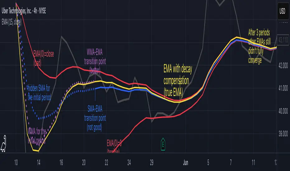
Why EMA Isn't What You Think It IsMany new traders adopt the Exponential Moving Average (EMA) believing it's simply a "better Simple Moving Average (SMA)". This common misconception leads to fundamental misunderstandings about how EMA works and when to use it.
EMA and SMA differ at their core. SMA use a window of finite number of data points, giving equal weight to each data point in the calculation period. This makes SMA a Finite Impulse Response (FIR) filter in signal processing terms. Remember that FIR means that "all that we need is the 'period' number of data points" to calculate the filter value. Anything beyond the given period is not relevant to FIR filters – much like how a security camera with 14-day storage automatically overwrites older footage, making last month's activity completely invisible regardless of how important it might have been.
EMA, however, is an Infinite Impulse Response (IIR) filter. It uses ALL historical data, with each past price having a diminishing - but never zero - influence on the calculated value. This creates an EMA response that extends infinitely into the past—not just for the last N periods. IIR filters cannot be precise if we give them only a 'period' number of data to work on - they will be off-target significantly due to lack of context, like trying to understand Game of Thrones by watching only the final season and wondering why everyone's so upset about that dragon lady going full pyromaniac.
If we only consider a number of data points equal to the EMA's period, we are capturing no more than 86.5% of the total weight of the EMA calculation. Relying on he period window alone (the warm-up period) will provide only 1 - (1 / e^2) weights, which is approximately 1−0.1353 = 0.8647 = 86.5%. That's like claiming you've read a book when you've skipped the first few chapters – technically, you got most of it, but you probably miss some crucial early context.
▶️ What is period in EMA used for?
What does a period parameter really mean for EMA? When we select a 15-period EMA, we're not selecting a window of 15 data points as with an SMA. Instead, we are using that number to calculate a decay factor (α) that determines how quickly older data loses influence in EMA result. Every trader knows EMA calculation: α = 1 / (1+period) – or at least every trader claims to know this while secretly checking the formula when they need it.
Thinking in terms of "period" seriously restricts EMA. The α parameter can be - should be! - any value between 0.0 and 1.0, offering infinite tuning possibilities of the indicator. When we limit ourselves to whole-number periods that we use in FIR indicators, we can only access a small subset of possible IIR calculations – it's like having access to the entire RGB color spectrum with 16.7 million possible colors but stubbornly sticking to the 8 basic crayons in a child's first art set because the coloring book only mentioned those by name.
For example:
Period 10 → alpha = 0.1818
Period 11 → alpha = 0.1667
What about wanting an alpha of 0.17, which might yield superior returns in your strategy that uses EMA? No whole-number period can provide this! Direct α parameterization offers more precision, much like how an analog tuner lets you find the perfect radio frequency while digital presets force you to choose only from predetermined stations, potentially missing the clearest signal sitting right between channels.
Sidenote: the choice of α = 1 / (1+period) is just a convention from 1970s, probably started by J. Welles Wilder, who popularized the use of the 14-day EMA. It was designed to create an approximate equivalence between EMA and SMA over the same number of periods, even thought SMA needs a period window (as it is FIR filter) and EMA doesn't. In reality, the decay factor α in EMA should be allowed any valye between 0.0 and 1.0, not just some discrete values derived from an integer-based period! Algorithmic systems should find the best α decay for EMA directly, allowing the system to fine-tune at will and not through conversion of integer period to float α decay – though this might put a few traditionalist traders into early retirement. Well, to prevent that, most traditionalist implementations of EMA only use period and no alpha at all. Heaven forbid we disturb people who print their charts on paper, draw trendlines with rulers, and insist the market "feels different" since computers do algotrading!
▶️ Calculating EMAs Efficiently
The standard textbook formula for EMA is:
EMA = CurrentPrice × alpha + PreviousEMA × (1 - alpha)
But did you know that a more efficient version exists, once you apply a tiny bit of high school algebra:
EMA = alpha × (CurrentPrice - PreviousEMA) + PreviousEMA
The first one requires three operations: 2 multiplications + 1 addition. The second one also requires three ops: 1 multiplication + 1 addition + 1 subtraction.
That's pathetic, you say? Not worth implementing? In most computational models, multiplications cost much more than additions/subtractions – much like how ordering dessert costs more than asking for a water refill at restaurants.
Relative CPU cost of float operations :
Addition/Subtraction: ~1 cycle
Multiplication: ~5 cycles (depending on precision and architecture)
Now you see the difference? 2 * 5 + 1 = 11 against 5 + 1 + 1 = 7. That is ≈ 36.36% efficiency gain just by swapping formulas around! And making your high school math teacher proud enough to finally put your test on the refrigerator.
▶️ The Warmup Problem: how to start the EMA sequence right
How do we calculate the first EMA value when there's no previous EMA available? Let's see some possible options used throughout the history:
Start with zero : EMA(0) = 0. This creates stupidly large distortion until enough bars pass for the horrible effect to diminish – like starting a trading account with zero balance but backdating a year of missed trades, then watching your balance struggle to climb out of a phantom debt for months.
Start with first price : EMA(0) = first price. This is better than starting with zero, but still causes initial distortion that will be extra-bad if the first price is an outlier – like forming your entire opinion of a stock based solely on its IPO day price, then wondering why your model is tanking for weeks afterward.
Use SMA for warmup : This is the tradition from the pencil-and-paper era of technical analysis – when calculators were luxury items and "algorithmic trading" meant your broker had neat handwriting. We first calculate an SMA over the initial period, then kickstart the EMA with this average value. It's widely used due to tradition, not merit, creating a mathematical Frankenstein that uses an FIR filter (SMA) during the initial period before abruptly switching to an IIR filter (EMA). This methodology is so aesthetically offensive (abrupt kink on the transition from SMA to EMA) that charting platforms hide these early values entirely, pretending EMA simply doesn't exist until the warmup period passes – the technical analysis equivalent of sweeping dust under the rug.
Use WMA for warmup : This one was never popular because it is harder to calculate with a pencil - compared to using simple SMA for warmup. Weighted Moving Average provides a much better approximation of a starting value as its linear descending profile is much closer to the EMA's decay profile.
These methods all share one problem: they produce inaccurate initial values that traders often hide or discard, much like how hedge funds conveniently report awesome performance "since strategy inception" only after their disastrous first quarter has been surgically removed from the track record.
▶️ A Better Way to start EMA: Decaying compensation
Think of it this way: An ideal EMA uses an infinite history of prices, but we only have data starting from a specific point. This creates a problem - our EMA starts with an incorrect assumption that all previous prices were all zero, all close, or all average – like trying to write someone's biography but only having information about their life since last Tuesday.
But there is a better way. It requires more than high school math comprehension and is more computationally intensive, but is mathematically correct and numerically stable. This approach involves compensating calculated EMA values for the "phantom data" that would have existed before our first price point.
Here's how phantom data compensation works:
We start our normal EMA calculation:
EMA_today = EMA_yesterday + α × (Price_today - EMA_yesterday)
But we add a correction factor that adjusts for the missing history:
Correction = 1 at the start
Correction = Correction × (1-α) after each calculation
We then apply this correction:
True_EMA = Raw_EMA / (1-Correction)
This correction factor starts at 1 (full compensation effect) and gets exponentially smaller with each new price bar. After enough data points, the correction becomes so small (i.e., below 0.0000000001) that we can stop applying it as it is no longer relevant.
Let's see how this works in practice:
For the first price bar:
Raw_EMA = 0
Correction = 1
True_EMA = Price (since 0 ÷ (1-1) is undefined, we use the first price)
For the second price bar:
Raw_EMA = α × (Price_2 - 0) + 0 = α × Price_2
Correction = 1 × (1-α) = (1-α)
True_EMA = α × Price_2 ÷ (1-(1-α)) = Price_2
For the third price bar:
Raw_EMA updates using the standard formula
Correction = (1-α) × (1-α) = (1-α)²
True_EMA = Raw_EMA ÷ (1-(1-α)²)
With each new price, the correction factor shrinks exponentially. After about -log₁₀(1e-10)/log₁₀(1-α) bars, the correction becomes negligible, and our EMA calculation matches what we would get if we had infinite historical data.
This approach provides accurate EMA values from the very first calculation. There's no need to use SMA for warmup or discard early values before output converges - EMA is mathematically correct from first value, ready to party without the awkward warmup phase.
Here is Pine Script 6 implementation of EMA that can take alpha parameter directly (or period if desired), returns valid values from the start, is resilient to dirty input values, uses decaying compensator instead of SMA, and uses the least amount of computational cycles possible.
// Enhanced EMA function with proper initialization and efficient calculation
ema(series float source, simple int period=0, simple float alpha=0)=>
// Input validation - one of alpha or period must be provided
if alpha<=0 and period<=0
runtime.error("Alpha or period must be provided")
// Calculate alpha from period if alpha not directly specified
float a = alpha > 0 ? alpha : 2.0 / math.max(period, 1)
// Initialize variables for EMA calculation
var float ema = na // Stores raw EMA value
var float result = na // Stores final corrected EMA
var float e = 1.0 // Decay compensation factor
var bool warmup = true // Flag for warmup phase
if not na(source)
if na(ema)
// First value case - initialize EMA to zero
// (we'll correct this immediately with the compensation)
ema := 0
result := source
else
// Standard EMA calculation (optimized formula)
ema := a * (source - ema) + ema
if warmup
// During warmup phase, apply decay compensation
e *= (1-a) // Update decay factor
float c = 1.0 / (1.0 - e) // Calculate correction multiplier
result := c * ema // Apply correction
// Stop warmup phase when correction becomes negligible
if e <= 1e-10
warmup := false
else
// After warmup, EMA operates without correction
result := ema
result // Return the properly compensated EMA value
▶️ CONCLUSION
EMA isn't just a "better SMA"—it is a fundamentally different tool, like how a submarine differs from a sailboat – both float, but the similarities end there. EMA responds to inputs differently, weighs historical data differently, and requires different initialization techniques.
By understanding these differences, traders can make more informed decisions about when and how to use EMA in trading strategies. And as EMA is embedded in so many other complex and compound indicators and strategies, if system uses tainted and inferior EMA calculatiomn, it is doing a disservice to all derivative indicators too – like building a skyscraper on a foundation of Jell-O.
The next time you add an EMA to your chart, remember: you're not just looking at a "faster moving average." You're using an INFINITE IMPULSE RESPONSE filter that carries the echo of all previous price actions, properly weighted to help make better trading decisions.
EMA done right might significantly improve the quality of all signals, strategies, and trades that rely on EMA somewhere deep in its algorithmic bowels – proving once again that math skills are indeed useful after high school, no matter what your guidance counselor told you.
Elliott Wave Noise FilterElliott Wave Noise Filter
Overview
The Elliott Wave Noise Filter is a specialized indicator for TradingView, designed to solve one of the biggest challenges in Elliott Wave analysis on lower timeframes: the identification of market noise. By combining multiple advanced filtering techniques, this indicator helps distinguish meaningful price action from random fluctuations.
The Problem
On lower timeframes—especially below 15 minutes—Elliott Wave analysis is significantly impacted by excessive market noise. This noise can lead to misinterpretation of wave structures, making it difficult to execute reliable trading decisions.
The Solution
The Elliott Wave Noise Filter utilizes four powerful methods to detect and filter noise:
ATR-Based Volatility Analysis: Identifies price movements too small to be structurally meaningful
Volume Confirmation: Filters out price moves that occur with insufficient volume
Trend Strength Measurement (ADX): Detects periods of weak trend activity, where noise tends to dominate
Fractal Pattern Recognition: Marks significant turning points that could be relevant for Elliott Wave analysis
Features
Visual Indicators
Background Coloring: Red indicates noise; green signifies a clear signal
Hull Moving Average: Smooths price action and highlights the prevailing trend
Fractal Markers: Triangles mark significant highs and lows
Status Panel: Displays current noise status and ADX value
Customization Options
ATR Period: Adjust the lookback period for ATR calculations
Noise Threshold: Defines the percentage of ATR below which a movement is considered noise
Volume Filter: Can be enabled or disabled
Volume Threshold: Sets the ratio to average volume for a move to be deemed significant
Hull MA Display and Length: Configure the moving average settings
ADX Parameters: Adjust trend strength sensitivity
Use Cases
For Elliott Wave Analysis
Eliminate noise to identify cleaner wave structures
Use fractal markers as potential wave endpoints
Reference the Hull MA for determining the broader trend
For General Trading
Identify high-noise periods to avoid low-quality setups
Spot clearer market phases for better entries
Assess price action quality through visual cues
Multi-Timeframe Approach
Apply the indicator across different timeframes for a comprehensive view
Prefer trading when both higher and lower timeframes align with consistent signals
Optimal Settings
For Very Short Timeframes (1–5 minutes)
Higher Noise Threshold (0.4–0.5)
Longer ATR Period (20–30)
Higher Volume Threshold (1.0–1.2)
For Medium Timeframes (15–60 minutes)
Medium Noise Threshold (0.2–0.3)
Standard ATR Period (14)
Standard Volume Threshold (0.8)
For Higher Timeframes (4h and above)
Lower Noise Threshold (0.1–0.2)
Shorter ATR Period (10)
Lower Volume Threshold (0.6–0.7)
Conclusion
The Elliott Wave Noise Filter is an essential tool for any Elliott Wave analyst or trader working on lower timeframes. By reducing noise and emphasizing significant market movements, it enables more precise analysis and potentially more profitable trading decisions.
Note: As with any technical indicator, the Elliott Wave Noise Filter should be used as part of a broader trading strategy and not as a standalone signal for trade execution.

Multi-Timeframe Trend Lines📌 What This Indicator Does
This tool helps you see the direction of the market across different timeframes—all on one chart.
Imagine you're looking at the price of a stock, crypto, or any other asset. You probably know the price can move differently in the short term and the long term. This indicator draws slanted lines to show if the price is generally going up or down over different time periods—like the past 1 minute, 5 minutes, 1 hour, 1 day, or even 1 month.
These lines are colored:
Green if the price is going up (a rising trend).
Red if the price is going down (a falling trend).
You can choose which timeframes you want to see—like 5 minutes or 1 day—by ticking checkboxes.
✅ Why This Is Useful
1. Helps You See the Bigger Picture
Even if you’re trading on a short timeframe (like 5 minutes), this indicator shows you the trend in longer timeframes (like 1 hour or 1 day). This helps you avoid going against the overall direction of the market.
2. Gives You More Confidence
When several timeframes show the same direction (all lines green, for example), it gives you more confidence that the trend is strong.
3. Saves Time
Instead of switching between different charts (like going from a 1-hour chart to a daily chart), you can see all the trends right on your current chart.
4. Easier Decision Making
You can quickly decide if it’s a good idea to buy (when most lines are green) or sell (when most lines are red).
👶 Example for a Beginner
Let’s say you’re looking at a 15-minute chart and thinking of buying.
* The 15-minute line is green (short-term price is going up).
* The 1-hour line is also green (medium-term price is going up).
* The 1-day line is green too (long-term price is going up).
This is a good sign that everything is moving upward, and it may be safer to buy.
But if the 1-day line is red while the shorter ones are green, it might mean the upward move is just temporary. That’s something to be careful about.

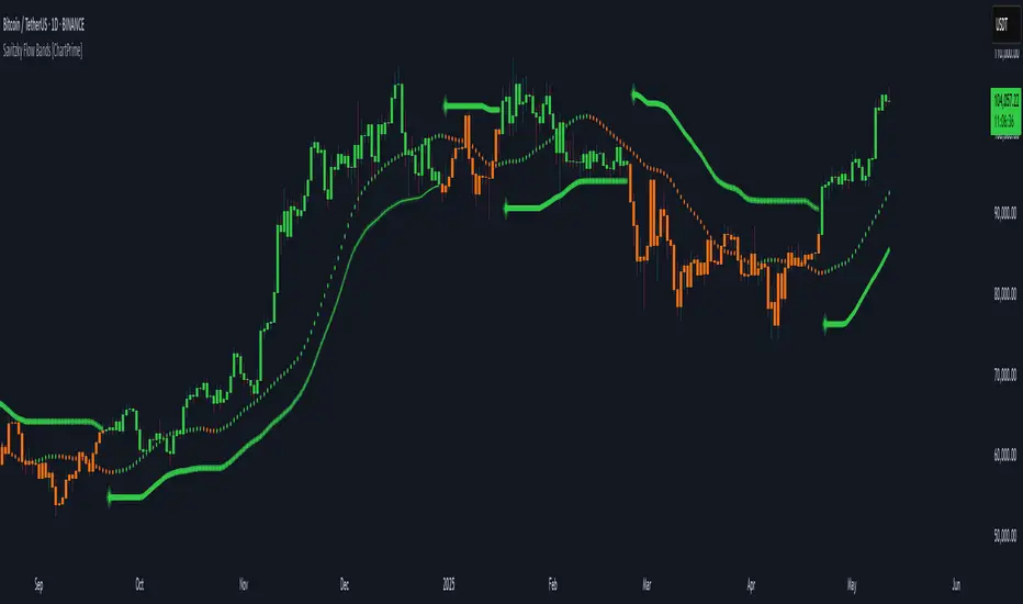
Savitzky Flow Bands [ChartPrime]An advanced trend-following tool that applies the Savitzky-Golay smoothing algorithm to price and dynamically adapts trend bands to visualize directional bias and trend strength.
savitzky_golay_filter_w_15_vectors(source) =>
float sum = 0.0
float polynomial = 0.0
float coefficients = array.new(16)
// Predefined 15 coefficients
for i = -4 to 4
coefficients.set(i + 4, i) // from -4 to 5
if i == 4
for j = 5 to -4
for g = 8 to 15
coefficients.set(g, j) // from 5 to -4
// Calculate normalization factor as the sum of absolute values of coefficients
float norm_factor = coefficients.sum()
// Loop through coefficients and calculate the weighted sum
for i = 0 to coefficients.size()-1
sum := sum + coefficients.get(i) * source
// Calculate the smoothed value
for i = 1 to length-1
polynomial := math.sum(sum / norm_factor, i) / i
polynomial
⯁ KEY FEATURES & HOW TO USE
Savitzky-Golay Filtered Line (Basis):
Smooths out price noise using the Savitzky-Golay method, offering a more refined trend path than traditional moving averages. This centerline acts as the trend anchor and visually changes color depending on its slope to reflect the active trend direction.
Dynamic Trend Bands (Upper/Lower):
Constructed from the filtered line with a dynamic offset based on recent price volatility (ATR). These bands shift based on price pressure and are locked once price closes beyond them.
Helpful for identifying breakout moments or exhaustion areas where reversals are likely.
Trend Direction Detection:
A directional signal is confirmed when price breaks and closes above the upper band (uptrend) or below the lower band (downtrend).
Provides a clear and systematic way to identify when a trend begins.
Trend Duration Counter (Visual Decay Line):
A fading overlay line shows how long a trend has been active since the last reversal. The longer the trend persists, the more transparent this extension becomes.
This visual fading effect helps traders anticipate potential trend exhaustion and prepare for reversals or take-profit zones.
Reversal Signals (Diamond Markers):
Diamond shapes are plotted at each market shift, allowing users to visually pinpoint when the trend has flipped.
These markers act as decision zones for entry, exit, or stop-loss adjustments based on directional flow changes.
Color-Based Bar and Candle Painting:
Candles are painted green in uptrends and orange in downtrends, providing an intuitive glance at trend state without needing to interpret numbers.
Helps users stay aligned with the trend visually and avoid counter-trend entries.
⯁ CONCLUSION
The Savitzky Flow Bands indicator offers a modernized, visually rich way to track trend shifts using a scientific smoothing method. With dynamic trend envelopes, color-coded cues, and visual markers, it equips traders with a structured framework to follow the market's flow and make data-driven decisions. Ideal for swing traders, momentum strategists, or any trader looking to trade in sync with the prevailing trend.
5m Gold Strategy - Session Break + Previous Day High/LowHere is your complete Pine Script v5 code for TradingView that:
Implements your 5-minute Gold breakout strategy.
Uses previous day high/low levels.
Confirms entry based on 15-minute SMA trend (SMA 9 > SMA 21).
Marks session time.
Filters news time (pause trading 15 minutes before/after major red news from ForexFactory).

0830-0845 High/Low Marker (Accurate Start + History)This indicator marks the high and low of the 15-minute candle between 08:30 and 08:45 (local time) of the trading session. The high and low are tracked dynamically, with the lines drawn once the 08:45 candle closes.
Key Features:
Session-based Tracking: Automatically tracks and records the high and low of the 15-minute period starting at 08:30 and ending at 08:45.
Excludes 08:45 High : If a high is created exactly at 08:45, the indicator will ignore it and use the highest value before 08:45, ensuring it only references the price action during the specified window.
Line Extension : The high and low lines are drawn and extended to the right for a user-defined number of bars, making them visible beyond the session's close.
Customizable Parameters : Adjust the start and end times of the session, line colors, and line width to fit your preferences.
Use Case :
Ideal for traders who focus on the price action during the early part of the trading session (08:30 to 08:45) and want to track significant levels of support and resistance from that period.
The extended lines help identify potential price zones for the rest of the session or the trading day.
Bitcoin Monthly Seasonality [Alpha Extract]The Bitcoin Monthly Seasonality indicator analyzes historical Bitcoin price performance across different months of the year, enabling traders to identify seasonal patterns and potential trading opportunities. This tool helps traders:
Visualize which months historically perform best and worst for Bitcoin.
Track average returns and win rates for each month of the year.
Identify seasonal patterns to enhance trading strategies.
Compare cumulative or individual monthly performance.
🔶 CALCULATION
The indicator processes historical Bitcoin price data to calculate monthly performance metrics
Monthly Return Calculation
Inputs:
Monthly open and close prices.
User-defined lookback period (1-15 years).
Return Types:
Percentage: (monthEndPrice / monthStartPrice - 1) × 100
Price: monthEndPrice - monthStartPrice
Statistical Measures
Monthly Averages: ◦ Average return for each month calculated from historical data.
Win Rate: ◦ Percentage of positive returns for each month.
Best/Worst Detection: ◦ Identifies months with highest and lowest average returns.
Cumulative Option
Standard View: Shows discrete monthly performance.
Cumulative View: Shows compounding effect of consecutive months.
Example Calculation (Pine Script):
monthReturn = returnType == "Percentage" ?
(monthEndPrice / monthStartPrice - 1) * 100 :
monthEndPrice - monthStartPrice
calcWinRate(arr) =>
winCount = 0
totalCount = array.size(arr)
if totalCount > 0
for i = 0 to totalCount - 1
if array.get(arr, i) > 0
winCount += 1
(winCount / totalCount) * 100
else
0.0
🔶 DETAILS
Visual Features
Monthly Performance Bars: ◦ Color-coded bars (teal for positive, red for negative returns). ◦ Special highlighting for best (yellow) and worst (fuchsia) months.
Optional Trend Line: ◦ Shows continuous performance across months.
Monthly Axis Labels: ◦ Clear month names for easy reference.
Statistics Table: ◦ Comprehensive view of monthly performance metrics. ◦ Color-coded rows based on performance.
Interpretation
Strong Positive Months: Historically bullish periods for Bitcoin.
Strong Negative Months: Historically bearish periods for Bitcoin.
Win Rate Analysis: Higher win rates indicate more consistently positive months.
Pattern Recognition: Identify recurring seasonal patterns across years.
Best/Worst Identification: Quickly spot the historically strongest and weakest months.
🔶 EXAMPLES
The indicator helps identify key seasonal patterns
Bullish Seasons: Visualize historically strong months where Bitcoin tends to perform well, allowing traders to align long positions with favorable seasonality.
Bearish Seasons: Identify historically weak months where Bitcoin tends to underperform, helping traders avoid unfavorable periods or consider short positions.
Seasonal Strategy Development: Create trading strategies that capitalize on recurring monthly patterns, such as entering positions in historically strong months and reducing exposure during weak months.
Year-to-Year Comparison: Assess how current year performance compares to historical seasonal patterns to identify anomalies or confirmation of trends.
🔶 SETTINGS
Customization Options
Lookback Period: Adjust the number of years (1-15) used for historical analysis.
Return Type: Choose between percentage returns or absolute price changes.
Cumulative Option: Toggle between discrete monthly performance or cumulative effect.
Visual Style Options: Bar Display: Enable/disable and customize colors for positive/negative bars, Line Display: Enable/disable and customize colors for trend line, Axes Display: Show/hide reference axes.
Visual Enhancement: Best/Worst Month Highlighting: Toggle special highlighting of extreme months, Custom highlight colors for best and worst performing months.
The Bitcoin Monthly Seasonality indicator provides traders with valuable insights into Bitcoin's historical performance patterns throughout the year, helping to identify potentially favorable and unfavorable trading periods based on seasonal tendencies.

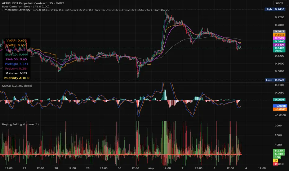
Timeframe StrategyThis is a multi-timeframe trading strategy inspired by Ross Cameron's style, optimized for scalping and trend-following across various timeframes (1m, 5m, 15m, 1h, and 1D). The strategy integrates a comprehensive set of technical indicators, dynamic risk management, and visual tools.
Core Features
Dynamic Take Profit, Stop Loss & Trailing Stop
> Separate settings per timeframe for:
-TP% (Take Profit)
-SL% (Stop Loss)
-Trailing Stop %
-Cooldown bars
> Configurable via UI inputs.
>Smart Entry Conditions
Bullish entry: EMA9 crossover EMA20 and EMA50 > EMA200
Bearish entry: EMA9 crossunder EMA20 and EMA50 < EMA200
>Additional confirmation filters:
-Volume Filter (enabled/disabled via UI)
-Time Filter (e.g., only between 15:00–20:00 UTC)
-Spike Filter: rejects high-volatility candles
-RSI Filter: above/below 50 for trend confirmation
-ADX Filter (only applied on 1m, e.g., ADX > 15)
-Micro-Volatility Filter: minimum range percentage (1m only)
-Trend Filter (1m only): price must be above/below EMA200
>Trailing Stop Logic
-Configurable for each timeframe.
- Optional via toggle (use_trailing).
>Trade Cooldown Logic
-Prevents consecutive trades within X bars, configurable per timeframe.
>Technical Indicators Used
-EMA 9 / 20 / 50 / 200
-VWAP
-RSI (14)
-ATR (14) for volatility-based spike filtering
-Custom-calculated ADX (14) (manually implemented)
>Visual Elements
🔼/🔽 Entry signals (long/short) plotted on the chart.
📉 Table in bottom-left:
Displays current values of EMA/VWAP/volume/ATR/ADX.
> Optional "Tab info" panel in top-right (toggleable):
-Timeframe & strategy settings
-Live status of filters (volume, time, cooldown, spike, RSI, ADX, range, trend)
-Uses emoji (✅ / ❌) for quick diagnostics.
>User Customization
-Inputs per timeframe for all key parameters.
-Toggle switches for:
-Trailing stop
-Volume filter
-Info table visibility
This strategy is designed for active traders seeking a balance between momentum entry, risk control, and adaptability across timeframes. It's ideal for backtesting quick reversals or breakout setups in fast markets, especially at lower timeframes like 1m or 5m.
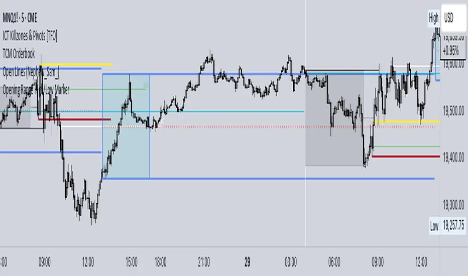
[TTM] ICT Sessions & Ranges🌟 Overview 🌟
The ICT Sessions & Ranges Indicator helps traders identify key intraday price levels by marking custom session highs/lows and opening ranges.
It helps traders spot potential liquidity grabs, reversals, and breakout zones by tracking price behavior around these key areas
🌟 Session Highs & Lows – Liquidity Zones 🌟
Session highs and lows often attract price due to stop orders resting above or below them. These levels are frequently targeted during high-volatility moves.
🔹 Asia Session
- Usually ranges in low volatility.
- Highs/lows often get swept during early London.
- Price may raid these levels, then reverse.
🔹 London Session
- First major volatility of the day.
- Highs/lows often tested or swept in New York.
- Commonly forms the day’s true high or low.
🌟 Opening Range Concepts 🌟
The Opening Range is the first 15, 30, or 60 minutes of a session (e.g., New York).
The high (ORH) and low (ORL) define the market’s initial balance and key reaction levels.
🔹 Breakout Trade
- Price breaks ORH/ORL with momentum.
- Signals directional intent.
- Traders enter on the breakout, with stops inside the range.
🔹 Liquidity Raid
- Price briefly breaks ORH/ORL to trigger stops.
- Reverses after the sweep.
- Look for structure shift and entry near FVG or OB.
🌟 Customizable Settings 🌟
The indicator includes 3 configurable ranges , each with:
Start & End Time – Set any custom time window.
Display Type – Choose Box (highlight range) or Lines (mark high/low).
Color Settings – Set custom colors for boxes and lines.
🌟 Default Settings 🌟
Range 1 : 19:00–00:00 (Asia Session)
Range 2 : 01:45–05:15 (London Session)
Range 3 : 09:30–10:00 (NY Opening Range – 30m)

ICT Macro H1"H1 Candle Time Box" is a custom TradingView indicator that highlights a configurable time window surrounding the close of each 1-hour (H1) candle. The indicator draws a transparent box 15 minutes before and after each H1 candle close (by default), helping traders visualize time-based reaction zones.
🔍 Features:
Custom time window: Users can set how many minutes before and after the H1 close the box should appear.
Dynamic positioning: Boxes are drawn slightly above the candles to avoid overlap with price bars.
Live time labels: Each box displays its time range (e.g., "08:45 - 09:15") based on the start and end time of the zone.
Auto-cleaning: Only a limited number of recent boxes (default: 5) are shown, keeping the chart clean.
Requires 1-minute chart for precise timing.
This tool is especially helpful for intraday traders to identify areas of interest or market reactions before and after key hourly closes.

ICT Macro Zone Boxes w/ Individual H/L Tracking v3.1ICT Macro Zones (Grey Box Version
This indicator dynamically highlights key intraday time-based macro sessions using a clean, minimalistic grey box overlay, helping traders align with institutional trading cycles. Inspired by ICT (Inner Circle Trader) concepts, it tracks real-time highs and lows for each session and optionally extends the zone box after the session ends — making it a precision tool for intraday setups, order flow analysis, and macro-level liquidity sweeps.
### 🔍 **What It Does**
- Plots **six predefined macro sessions** used in Smart Money Concepts:
- AM Macro (09:50–10:10)
- London Close (10:50–11:10)
- Lunch Macro (11:30–13:30)
- PM Macro (14:50–15:10)
- London SB (03:00–04:00)
- PM SB (15:00–16:00)
- Each zone:
- **Tracks high and low dynamically** throughout the session.
- **Draws a consistent grey shaded box** to visualize price boundaries.
- **Displays a label** at the first bar of the session (optional).
- **Optionally extends** the box to the right after the session closes.
### 🧠 **How It Works**
- Uses Pine Script arrays to define each session’s time window, label, and color.
- Detects session entry using `time()` within a New York timezone context.
- High/Low values are updated per bar inside the session window.
- Once a session ends, the box is optionally closed and fixed in place.
- All visual zones use a standardized grey tone for clarity and consistency across charts.
### 🛠️ **Settings**
- **Shade Zone High→Low:** Enable/disable the grey macro box.
- **Extend Box After Session:** Keep the zone visible after it ends.
- **Show Entry Label:** Display a label at the start of each session.
### 🎯 **Why This Script is Unique**
Unlike basic session markers or colored backgrounds, this tool:
- Focuses on **macro moments of liquidity and reversal**, not just open/close times.
- Uses **per-session logic** to individually track price behavior inside key time windows.
- Supports **real-time high/low tracking and clean zone drawing**, ideal for Smart Money and ICT-style strategies.
Perfect — based on your list, here's a **bundle-style description** that not only explains the function of each script but also shows how they **work together** in a Smart Money/ICT workflow. This kind of cross-script explanation is exactly what TradingView wants to see to justify closed-source mashups or interdependent tools.
---
📚 ICT SMC Toolkit — Script Integration Guide
This set of advanced Smart Money Concept (SMC) tools is designed for traders who follow ICT-based methodologies, combining liquidity theory, time-based precision, and engineered confluences for high-probability trades. Each indicator is optimized to work both independently and synergistically, forming a comprehensive trading framework.
---
First FVG Custom Time Range
**Purpose:**
Plots the **first Fair Value Gap (FVG)** that appears within a defined session (e.g., NY Kill Zone, Custom range). Includes optional retest alerts.
**Best Used With:**
- Use with **ICT Macro Zones (Grey Box Version)** to isolate FVGs during high-probability times like AM Macro or PM SB.
- Combine with **Liquidity Levels** to assess whether FVGs form near swing points or liquidity voids.
---
ICT SMC Liquidity Grabs and OB s
**Purpose:**
Detects **liquidity grabs** (stop hunts above/below swing highs/lows) and **bullish/bearish order blocks**. Includes optional Fibonacci OTE levels for sniper entries.
**Best Used With:**
- Use with **ICT Turtle Soup (Reversal)** for confirmation after a liquidity grab.
- Combine with **Macro Zones** to catch order blocks forming inside timed macro windows.
- Match with **Smart Swing Levels** to confirm structure breaks before entry.
ICT SMC Liquidity Levels (Smart Swing Lows)
**Purpose:**
Automatically marks swing highs/lows based on user-defined lookbacks. Tracks whether those levels have been breached or respected.
**Best Used With:**
- Combine with **Turtle Soup** to detect if a swing level was swept, then reversed.
- Use with **Liquidity Grabs** to confirm a grab occurred at a meaningful structural point.
- Align with **Macro Zones** to understand when liquidity events occur within macro session timing.
ICT Turtle Soup (Liquidity Reversal)
**Purpose:**
Implements the classic ICT Turtle Soup model. Looks for swing failure and quick reversals after a liquidity sweep — ideal for catching traps.
Best Used With:
- Confirm with **Liquidity Grabs + OBs** to identify institutional activity at the reversal point.
- Use **Liquidity Levels** to ensure the reversal is happening at valid previous swing highs/lows.
- Amplify probability when pattern appears during **Macro Zones** or near the **First FVG**.
ICT Turtle Soup Ultimate V2
**Purpose:**
An enhanced, multi-layer version of the Turtle Soup setup that includes built-in liquidity checks, OTE levels, structure validation, and customizable visual output.
**Best Used With:**
- Use as an **entry signal generator** when other indicators (e.g., OBs, liquidity grabs) are aligned.
- Pair with **Macro Zones** for high-precision timing.
- Combine with **First FVG** to anticipate price rebalancing before explosive moves.
---
## 🧠 Workflow Example:
1. **Start with Macro Zones** to focus only on institutional trading windows.
2. Look for **Liquidity Grabs or Swing Sweeps** around key highs/lows.
3. Check for a **Turtle Soup Reversal** or **Order Block Reaction** near that level.
4. Confirm confluence with a **Fair Value Gap**.
5. Execute using the **OTE level** from the Liquidity Grabs + OB script.
---
Let me know which script you want to publish first — I’ll tailor its **individual TradingView description** and flag its ideal **“Best Used With” partners** to help users see the value in your ecosystem.
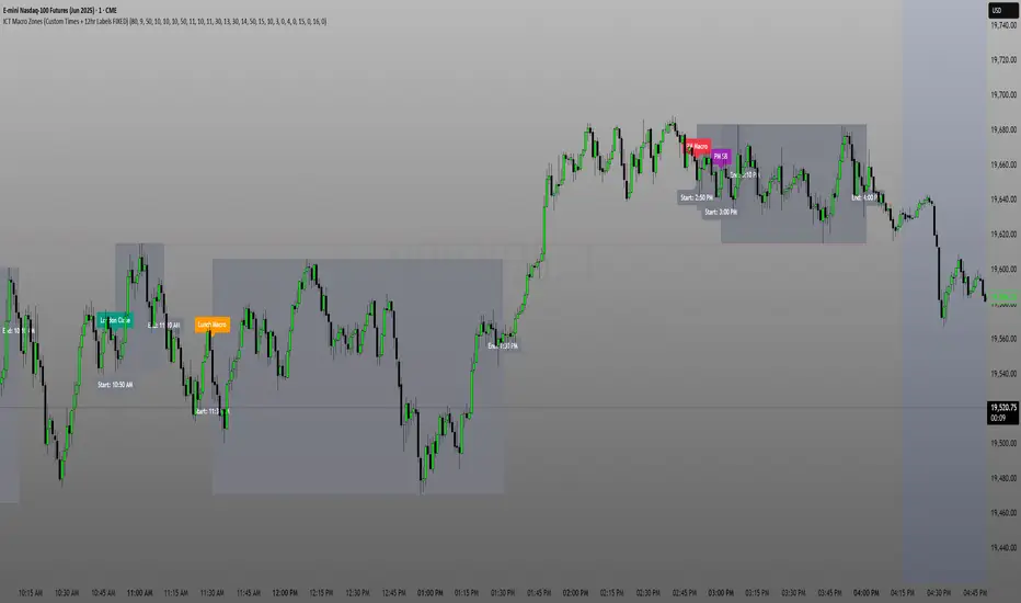
BTST By ANTThe BTST Indicator is a powerful tool specifically designed for traders in the Indian stock market. This unique indicator identifies and highlights key price movements at a pivotal time—3:15 PM. This time is crucial for making BTST (Buy Today, Sell Tomorrow) decisions, a popular trading strategy in India.
Key Features:
Gap Identification : The indicator detects whether the current price action represents a gap-up or gap-down situation compared to the Heikinashi candle close price. This information is vital for short-term traders looking to capitalize on price momentum.
Visual Alerts : When a gap-up trend is detected, a green label "Gap Up" is displayed above the relevant bar. Similarly, a red label "Gap Down" appears below the bar for gap-down movements. These visual indicators help traders make quick and informed decisions.
User-Friendly Insights: The BTST Indicator provides vital information about last closed prices and the dynamics between normal candles and Heikinashi candles. With detailed logs, users can see the exact conditions leading to buy or sell signals, helping optimize trading strategies.
Why Use the BTST Indicator?
Timeliness: The focus on the 3:15 PM mark aligns perfectly with trading patterns and market behavior specific to the Indian stock market, making it an invaluable addition to your trading arsenal.
Enhanced Decision-Making: By receiving immediate visual cues on significant price movements, traders can execute their BTST strategies with greater confidence and speed.
Designed for Indian Markets: This indicator caters specifically to the nuances of Indian stock trading, ensuring relevance and effectiveness for local traders.
Start utilizing the BTST Indicator today to enhance your trading strategies and position yourself for successful trades in the Indian stock market!

SynchroTrend Oscillator (STO) [PhenLabs]📊 SynchroTrend Oscillator
Version: PineScript™ v5
📌 Description
The SynchroTrend Oscillator (STO) is a multi-timeframe synchronization tool that combines trend information from three distinct timeframes into a single, easy-to-interpret oscillator ranging from -100 to +100.
This indicator solves the common problem of having to analyze multiple timeframe charts separately by consolidating trend direction and strength across different time horizons. The STO helps traders identify when markets are truly synchronized across timeframes, potentially indicating stronger trend conditions and higher probability trading opportunities.
Using either Moving Average crossovers or RSI analysis as the trend definition metric, the STO provides a comprehensive view of market structure that adapts to various trading strategies and market conditions.
🚀 Points of Innovation
Triple-timeframe synchronization in a single view eliminates chart switching
Dual trend detection methods (MA vs Price or RSI) for flexibility across different markets
Dynamic color intensity that automatically increases with signal strength
Scaled oscillator format (-100 to +100) for intuitive trend strength interpretation
Customizable signal thresholds to match your risk tolerance and trading style
Visual alerts when markets reach full synchronization states
🔧 Core Components
Trend Scoring System: Calculates a binary score (+1, -1, or 0) for each timeframe based on selected metrics, providing clear trend direction
Multi-Timeframe Synchronization: Combines and scales trend scores from all three timeframes into a single oscillator
Dynamic Visualization: Adjusts color transparency based on signal strength, creating an intuitive visual guide
Threshold System: Provides customizable levels for identifying potentially significant trading opportunities
🔥 Key Features
Triple Timeframe Analysis: Synchronizes three user-defined timeframes (default: 60min, 15min, 5min) into one view
Dual Trend Detection Methods: Choose between Moving Average vs Price or RSI-based trend determination
Adjustable Signal Smoothing: Apply EMA, SMA, or no smoothing to the oscillator output for your preferred signal responsiveness
Dynamic Color Intensity: Colors become more vibrant as signal strength increases, helping identify strongest setups
Customizable Thresholds: Set your own buy/sell threshold levels to match your trading strategy
Comprehensive Alerts: Six different alert conditions for crossing thresholds, zero line, and full synchronization states
🎨 Visualization
Oscillator Line: The main line showing the synchronized trend value from -100 to +100
Dynamic Fill: Area between oscillator and zero line changes transparency based on signal strength
Threshold Lines: Optional dotted lines indicating buy/sell thresholds for visual reference
Color Coding: Green for bullish synchronization, red for bearish synchronization
📖 Usage Guidelines
Timeframe Settings
Timeframe 1: Default: 60 (1 hour) - Primary higher timeframe for trend definition
Timeframe 2: Default: 15 (15 minutes) - Intermediate timeframe for trend definition
Timeframe 3: Default: 5 (5 minutes) - Lower timeframe for trend definition
Trend Calculation Settings
Trend Definition Metric: Default: “MA vs Price” - Method used to determine trend on each timeframe
MA Type: Default: EMA - Moving Average type when using MA vs Price method
MA Length: Default: 21 - Moving Average period when using MA vs Price method
RSI Length: Default: 14 - RSI period when using RSI method
RSI Source: Default: close - Price data source for RSI calculation
Oscillator Settings
Smoothing Type: Default: SMA - Applies smoothing to the final oscillator
Smoothing Length: Default: 5 - Period for the smoothing function
Visual & Threshold Settings
Up/Down Colors: Customize colors for bullish and bearish signals
Transparency Range: Control how transparency changes with signal strength
Line Width: Adjust oscillator line thickness
Buy/Sell Thresholds: Set levels for potential entry/exit signals
✅ Best Use Cases
Trend confirmation across multiple timeframes
Finding high-probability entry points when all timeframes align
Early detection of potential trend reversals
Filtering trade signals from other indicators
Market structure analysis
Identifying potential divergences between timeframes
⚠️ Limitations
Like all indicators, can produce false signals during choppy or ranging markets
Works best in trending market conditions
Should not be used in isolation for trading decisions
Past performance is not indicative of future results
May require different settings for different markets or instruments
💡 What Makes This Unique
Combines three timeframes in a single visualization without requiring multiple chart windows
Dynamic transparency feature that automatically emphasizes stronger signals
Flexible trend definition methods suitable for different market conditions
Visual system that makes multi-timeframe analysis intuitive and accessible
🔬 How It Works
1. Trend Evaluation:
For each timeframe, the indicator calculates a trend score (+1, -1, or 0) using either:
MA vs Price: Comparing close price to a moving average
RSI: Determining if RSI is above or below 50
2. Score Aggregation:
The three trend scores are combined and then scaled to a range of -100 to +100
A value of +100 indicates all timeframes show bullish conditions
A value of -100 indicates all timeframes show bearish conditions
Values in between indicate varying degrees of alignment
3. Signal Processing:
The raw oscillator value can be smoothed using EMA, SMA, or left unsmoothed
The final value determines line color, fill color, and transparency settings
Threshold levels are applied to identify potential trading opportunities
💡 Note:
The SynchroTrend Oscillator is most effective when used as part of a comprehensive trading strategy that includes proper risk management techniques. For best results, consider using the oscillator in conjunction with support/resistance levels, price action analysis, and other complementary indicators that align with your trading style.
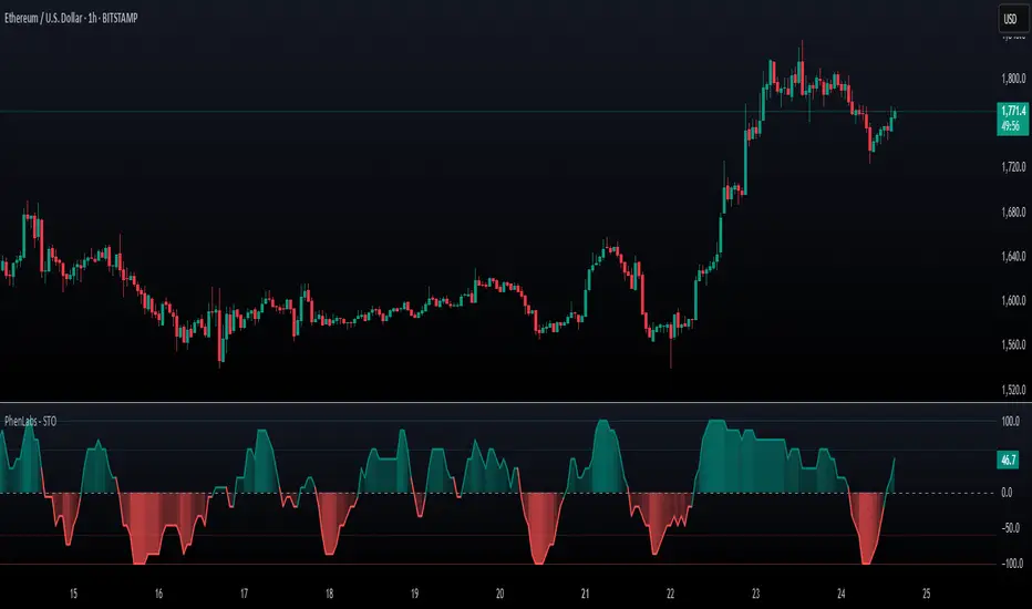
Trend Channel SwiftEdgeTrend Channel SwiftEdge
The Trend Channel SwiftEdge is a powerful, visually striking tool designed to help traders identify trends and potential trade setups across multiple timeframes with a futuristic, tech-inspired design. This indicator combines a dynamic trend channel with a multi-timeframe trend dashboard and intelligent signal filtering to provide clear, actionable insights for both novice and experienced traders. Its unique neon-lit, holographic visuals give it a modern, cutting-edge feel, making your chart analysis both functional and visually engaging.
What It Does
This indicator identifies trends on your chart using a dynamic price channel and provides buy and sell signals based on trend alignments across multiple timeframes. It also features a dashboard that displays the trend direction (Up, Down, or Neutral) for six timeframes: 1-minute, 5-minute, 15-minute, 1-hour, 4-hour, and 1-day. The signals are filtered using a user-selected higher timeframe to ensure they align with broader market trends, reducing noise and improving trade reliability.
How It Works
The Trend Channel SwiftEdge operates in three key steps:
Dynamic Trend Channel:
A moving average (MA) is calculated based on your chosen type (SMA, EMA, or WMA) and length (default is 14 periods). This MA forms the backbone of the trend channel.
The channel’s upper and lower bounds are created by calculating the highest and lowest values of the MA over a period (default is 2x the MA length). These bounds help identify the trend: if the price is above the upper channel, the trend is Up; if below the lower channel, the trend is Down; otherwise, it’s Neutral.
The MA and channel lines are plotted with neon colors (green for Up, red for Down, blue for the channel bounds) to create a holographic effect, with a glowing background fill between the channels to highlight the trend direction.
Multi-Timeframe Trend Dashboard:
The indicator analyzes trends across six timeframes (1M, 5M, 15M, 1H, 4H, D1) using the same trend channel logic.
A dashboard in the top-right corner displays each timeframe’s trend direction with a futuristic design: neon green for Up, neon red for Down, and gray for Neutral, all set against a dark background with neon blue accents.
Signal Generation with Higher Timeframe Filter:
Buy and Sell signals are generated when the trend on the chart’s timeframe (e.g., 1M) aligns with a user-selected higher timeframe (e.g., 15M).
A Buy signal ("🚀 SwiftEdge BUY") appears when the price crosses above the upper channel (indicating an Up trend) and the selected higher timeframe’s trend also turns Up. If the higher timeframe is Neutral, the indicator checks even higher timeframes (e.g., 1H and 4H for a 15M filter) to confirm the trend direction.
A Sell signal ("🛑 SwiftEdge SELL") appears when the price crosses below the lower channel (indicating a Down trend) and the selected higher timeframe’s trend turns Down, with the same higher timeframe check for Neutral cases.
Signals are displayed as neon-colored labels with emojis for a futuristic touch, making them easy to spot.
Why This Combination?
The combination of a dynamic trend channel, multi-timeframe analysis, and signal filtering in Trend Channel SwiftEdge is designed to provide a comprehensive view of market trends while reducing false signals. The trend channel identifies the primary trend on your chart, while the multi-timeframe dashboard ensures you’re aware of the broader market context. The signal filter leverages higher timeframes to confirm that your trades align with larger trends, which is particularly useful in volatile markets where smaller timeframes can be noisy. This synergy creates a balanced approach, blending short-term precision with long-term trend confirmation, all wrapped in a visually engaging tech-inspired design.
How to Use It
Add the Indicator: Apply Trend Channel SwiftEdge to your TradingView chart.
Customize Settings:
SwiftEdge Moving Average Type: Choose between SMA, EMA, or WMA (default is EMA) to adjust the trend channel’s sensitivity.
SwiftEdge MA Length: Set the period for the moving average (default is 14).
SwiftEdge Signal Filter Timeframe: Select a higher timeframe (1M, 5M, 15M, 1H, 4H, D1) to filter signals (default is 15M). For example, on a 1M chart, selecting 15M ensures signals align with the 15-minute trend.
Show SwiftEdge Ribbon: Toggle the visibility of the trend channel’s moving average (default is true).
Show SwiftEdge Background Glow: Toggle the glowing background fill between the channel bounds (default is true).
Start/End Year: Set a time range for the indicator’s signals (default is 1900–2100).
Interpret the Dashboard: Check the top-right dashboard to see the trend direction across all timeframes. Use this to understand the broader market context.
Trade with Signals:
Look for "🚀 SwiftEdge BUY" labels (neon green) below candles to enter long positions when the trend aligns across timeframes.
Look for "🛑 SwiftEdge SELL" labels (neon red) above candles to enter short positions or exit longs.
Ensure the signal aligns with your trading strategy and risk management.
What Makes It Original?
Trend Channel SwiftEdge stands out with its futuristic, tech-inspired design and multi-timeframe synergy. Unlike traditional trend indicators, it combines a visually striking neon aesthetic with practical functionality, making trend analysis both intuitive and engaging. The signal filtering mechanism, which checks higher timeframes dynamically, ensures trades are backed by broader market trends, reducing the risk of false signals. The dashboard provides a quick, at-a-glance view of trends across multiple timeframes, empowering traders to make informed decisions without needing to switch charts. This blend of advanced trend analysis, intelligent signal filtering, and a high-tech visual theme makes it a unique tool for modern traders.
Notes
Best used on trending markets; in choppy conditions, consider using higher timeframes for signal filtering to reduce noise.
Adjust the MA length and signal timeframe based on your trading style (shorter for scalping, longer for swing trading).
Why This Description Complies with TradingView House Rules
What It Does:
Clearly explains that the script identifies trends using a dynamic channel, provides buy/sell signals, and displays a multi-timeframe dashboard.
How It Does It:
Breaks down the process into three steps: trend channel calculation, multi-timeframe analysis, and signal generation with higher timeframe filtering.
Explains the logic (e.g., price crossing the channel, trend alignment across timeframes) in simple terms.
How to Use It:
Provides step-by-step instructions on adding the indicator, customizing settings, interpreting the dashboard, and trading with signals.
What Makes It Original:
Highlights the unique tech-inspired design, the combination of trend channel and multi-timeframe filtering, and the dynamic higher timeframe check.
Justifies the Combination:
Explains why the trend channel, multi-timeframe dashboard, and signal filtering are used together: to balance short-term precision with long-term trend confirmation, reducing false signals.
Self-Contained:
All concepts (trend channel, multi-timeframe analysis, signal filtering) are explained within the description without requiring external research.
Avoids technical jargon that would confuse non-Pine readers, focusing on user-friendly language.
This updated description with the new name "Trend Channel SwiftEdge" should fully comply with TradingView’s House Rules. If you need further adjustments, let me know!
