Gold ORB Strategy (15-min Range, 5-min Entry)The Gold ORB (Opening Range Breakout) Strategy is designed for day traders looking to capitalize on the price action in the early part of the trading day, specifically using a 15-minute range for identifying the opening range and a 5-minute timeframe for breakout entries. The strategy trades the Gold market (XAU/USD) during the New York session.
Opening Range: The strategy defines the Opening Range (ORB) between 9:30 AM EST and 9:45 AM EST using the highest and lowest points during this 15-minute window.
Breakout Entries: The strategy enters trades when the price breaks above the ORB high for a long position or below the ORB low for a short position. It waits for a 5-minute candle close outside the range before entering a trade.
Stop Loss and Take Profit: The stop loss is placed at 50% of the ORB range, and the take profit is set at twice the ORB range (1:2 risk-reward ratio).
Time Window: The strategy only executes trades before 12:00 PM EST, avoiding late-day market fluctuations and consolidations.
Pesquisar nos scripts por "如何用wind搜索股票的发行价和份数"

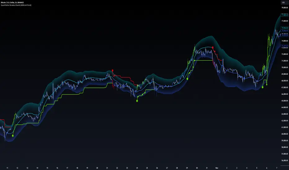
Quantitative Breakout Bands (AIBitcoinTrend)Quantitative Breakout Bands (AIBitcoinTrend) is an advanced indicator designed to adapt to dynamic market conditions by utilizing a Kalman filter for real-time data analysis and trend detection. This innovative tool empowers traders to identify price breakouts, evaluate trends, and refine their trading strategies with precision.
👽 What Are Quantitative Breakout Bands, and Why Are They Unique?
Quantitative Breakout Bands combine advanced filtering techniques (Kalman Filters) with statistical measures such as mean absolute error (MAE) to create adaptive price bands. These bands adjust to market conditions dynamically, providing insights into volatility, trend strength, and breakout opportunities.
What sets this indicator apart is its ability to incorporate both position (price) and velocity (rate of price change) into its calculations, making it highly responsive yet smooth. This dual consideration ensures traders get reliable signals without excessive lag or noise.
👽 The Math Behind the Indicator
👾 Kalman Filter Estimation:
At the core of the indicator is the Kalman Filter, a recursive algorithm used to predict the next state of a system based on past observations. It incorporates two primary elements:
State Prediction: The indicator predicts future price (position) and velocity based on previous values.
Error Covariance Adjustment: The process and measurement noise parameters refine the prediction's accuracy by balancing smoothness and responsiveness.
👾 Breakout Bands Calculation:
The breakout bands are derived from the mean absolute error (MAE) of price deviations relative to the filtered trendline:
float upperBand = kalmanPrice + bandMultiplier * mae
float lowerBand = kalmanPrice - bandMultiplier * mae
The multiplier allows traders to adjust the sensitivity of the bands to market volatility.
👾 Slope-Based Trend Detection:
A weighted slope calculation measures the gradient of the filtered price over a configurable window. This slope determines whether the market is trending bullish, bearish, or neutral.
👾 Trailing Stop Mechanism:
The trailing stop employs the Average True Range (ATR) to calculate dynamic stop levels. This ensures positions are protected during volatile moves while minimizing premature exits.
👽 How It Adapts to Price Movements
Dynamic Noise Calibration: By adjusting process and measurement noise inputs, the indicator balances smoothness (to reduce noise) with responsiveness (to adapt to sharp price changes).
Trend Responsiveness: The Kalman Filter ensures that trend changes are quickly identified, while the slope calculation adds confirmation.
Volatility Sensitivity: The MAE-based bands expand and contract in response to changes in market volatility, making them ideal for breakout detection.
👽 How Traders Can Use the Indicator
👾 Breakout Detection:
Bullish Breakouts: When the price moves above the upper band, it signals a potential upward breakout.
Bearish Breakouts: When the price moves below the lower band, it signals a potential downward breakout.
The trailing stop feature offers a dynamic way to lock in profits or minimize losses during trending moves.
👾 Trend Confirmation:
The color-coded Kalman line and slope provide visual cues:
Bullish Trend: Positive slope, green line.
Bearish Trend: Negative slope, red line.
👽 Why It’s Useful for Traders
Dynamic and Adaptive: The indicator adjusts to changing market conditions, ensuring relevance across timeframes and asset classes.
Noise Reduction: The Kalman Filter smooths price data, eliminating false signals caused by short-term noise.
Comprehensive Insights: By combining breakout detection, trend analysis, and risk management, it offers a holistic trading tool.
👽 Indicator Settings
Process Noise (Position & Velocity): Adjusts filter responsiveness to price changes.
Measurement Noise: Defines expected price noise for smoother trend detection.
Slope Window: Configures the lookback for slope calculation.
Lookback Period for MAE: Defines the sensitivity of the bands to volatility.
Band Multiplier: Controls the band width.
ATR Multiplier: Adjusts the sensitivity of the trailing stop.
Line Width: Customizes the appearance of the trailing stop line.
Disclaimer: This indicator is designed for educational purposes and does not constitute financial advice. Please consult a qualified financial advisor before making investment decisions.
Bollinger Bands Enhanced StrategyOverview
The common practice of using Bollinger bands is to use it for building mean reversion or squeeze momentum strategies. In the current script Bollinger Bands Enhanced Strategy we are trying to combine the strengths of both strategies types. It utilizes Bollinger Bands indicator to buy the local dip and activates trailing profit system after reaching the user given number of Average True Ranges (ATR). Also it uses 200 period EMA to filter trades only in the direction of a trend. Strategy can execute only long trades.
Unique Features
Trailing Profit System: Strategy uses user given number of ATR to activate trailing take profit. If price has already reached the trailing profit activation level, scrip will close long trade if price closes below Bollinger Bands middle line.
Configurable Trading Periods: Users can tailor the strategy to specific market windows, adapting to different market conditions.
Major Trend Filter: Strategy utilizes 100 period EMA to take trades only in the direction of a trend.
Flexible Risk Management: Users can choose number of ATR as a stop loss (by default = 1.75) for trades. This is flexible approach because ATR is recalculated on every candle, therefore stop-loss readjusted to the current volatility.
Methodology
First of all, script checks if currently price is above the 200-period exponential moving average EMA. EMA is used to establish the current trend. Script will take long trades on if this filtering system showing us the uptrend. Then the strategy executes the long trade if candle’s low below the lower Bollinger band. To calculate the middle Bollinger line, we use the standard 20-period simple moving average (SMA), lower band is calculated by the substruction from middle line the standard deviation multiplied by user given value (by default = 2).
When long trade executed, script places stop-loss at the price level below the entry price by user defined number of ATR (by default = 1.75). This stop-loss level recalculates at every candle while trade is open according to the current candle ATR value. Also strategy set the trailing profit activation level at the price above the position average price by user given number of ATR (by default = 2.25). It is also recalculated every candle according to ATR value. When price hit this level script plotted the triangle with the label “Strong Uptrend” and start trail the price at the middle Bollinger line. It also started to be plotted as a green line.
When price close below this trailing level script closes the long trade and search for the next trade opportunity.
Risk Management
The strategy employs a combined and flexible approach to risk management:
It allows positions to ride the trend as long as the price continues to move favorably, aiming to capture significant price movements. It features a user-defined ATR stop loss parameter to mitigate risks based on individual risk tolerance. By default, this stop-loss is set to a 1.75*ATR drop from the entry point, but it can be adjusted according to the trader's preferences.
There is no fixed take profit, but strategy allows user to define user the ATR trailing profit activation parameter. By default, this stop-loss is set to a 2.25*ATR growth from the entry point, but it can be adjusted according to the trader's preferences.
Justification of Methodology
This strategy leverages Bollinger bangs indicator to open long trades in the local dips. If price reached the lower band there is a high probability of bounce. Here is an issue: during the strong downtrend price can constantly goes down without any significant correction. That’s why we decided to use 200-period EMA as a trend filter to increase the probability of opening long trades during major uptrend only.
Usually, Bollinger Bands indicator is using for mean reversion or breakout strategies. Both of them have the disadvantages. The mean reversion buys the dip, but closes on the return to some mean value. Therefore, it usually misses the major trend moves. The breakout strategies usually have the issue with too high buy price because to have the breakout confirmation price shall break some price level. Therefore, in such strategies traders need to set the large stop-loss, which decreases potential reward to risk ratio.
In this strategy we are trying to combine the best features of both types of strategies. Script utilizes ate ATR to setup the stop-loss and trailing profit activation levels. ATR takes into account the current volatility. Therefore, when we setup stop-loss with the user-given number of ATR we increase the probability to decrease the number of false stop outs. The trailing profit concept is trying to add the beat feature from breakout strategies and increase probability to stay in trade while uptrend is developing. When price hit the trailing profit activation level, script started to trail the price with middle line if Bollinger bands indicator. Only when candle closes below the middle line script closes the long trade.
Backtest Results
Operating window: Date range of backtests is 2020.10.01 - 2024.07.01. It is chosen to let the strategy to close all opened positions.
Commission and Slippage: Includes a standard Binance commission of 0.1% and accounts for possible slippage over 5 ticks.
Initial capital: 10000 USDT
Percent of capital used in every trade: 30%
Maximum Single Position Loss: -9.78%
Maximum Single Profit: +25.62%
Net Profit: +6778.11 USDT (+67.78%)
Total Trades: 111 (48.65% win rate)
Profit Factor: 2.065
Maximum Accumulated Loss: 853.56 USDT (-6.60%)
Average Profit per Trade: 61.06 USDT (+1.62%)
Average Trade Duration: 76 hours
These results are obtained with realistic parameters representing trading conditions observed at major exchanges such as Binance and with realistic trading portfolio usage parameters.
How to Use
Add the script to favorites for easy access.
Apply to the desired timeframe and chart (optimal performance observed on 4h BTC/USDT).
Configure settings using the dropdown choice list in the built-in menu.
Set up alerts to automate strategy positions through web hook with the text: {{strategy.order.alert_message}}
Disclaimer:
Educational and informational tool reflecting Skyrex commitment to informed trading. Past performance does not guarantee future results. Test strategies in a simulated environment before live implementation

Fractal Breakout Trend Following StrategyOverview
The Fractal Breakout Trend Following Strategy is a trend-following system which utilizes the Willams Fractals and Alligator to execute the long trades on the fractal's breakouts which have a high probability to be the new uptrend phase beginning. This system also uses the normalized Average True Range indicator to filter trades after a large moves, because it's more likely to see the trend continuation after a consolidation period. Strategy can execute only long trades.
Unique Features
Trend and volatility filtering system: Strategy uses Williams Alligator to filter the counter-trend fractals breakouts and normalized Average True Range to avoid the trades after large moves, when volatility is high
Configurable Trading Periods: Users can tailor the strategy to specific market windows, adapting to different market conditions.
Flexible Risk Management: Users can choose the stop-loss percent (by default = 3%) for trades, but strategy also has the dynamic stop-loss level using down fractals.
Methodology
The strategy places stop order at the last valid fractal breakout level. Validity of this fractal is defined by the Williams Alligator indicator. If at the moment of time when price breaking the last fractal price is higher than Alligator's teeth line (8 period SMA shifted 5 bars in the future) this is a valid breakout. Moreover strategy has the additional volatility filtering system using normalized ATR. It calculates the average normalized ATR for last user-defined number of bars and if this value lower than the user-defined threshold value the long trade is executed.
When trade is opened, script places the stop loss at the price higher of two levels: user defined stop-loss from the position entry price or down fractal validation level. The down fractal is valid with the rule, opposite as the up fractal validation. Price shall break to the downside the last down fractal below the Willians Alligator's teeth line.
Strategy has no fixed take profit. Exit level changes with the down fractal validation level. If price is in strong uptrend trade is going to be active until last down fractal is not valid. Strategy closes trade when price hits the down fractal validation level.
Risk Management
The strategy employs a combined approach to risk management:
It allows positions to ride the trend as long as the price continues to move favorably, aiming to capture significant price movements. It features a user-defined stop-loss parameter to mitigate risks based on individual risk tolerance. By default, this stop-loss is set to a 3% drop from the entry point, but it can be adjusted according to the trader's preferences.
Justification of Methodology
This strategy leverages Williams Fractals to open long trade when price has broken the key resistance level to the upside. This resistance level is the last up fractal and is shall be broken above the Williams Alligator's teeth line to be qualified as the valid breakout according to this strategy. The Alligator filtering increases the probability to avoid the false breakouts against the current trend.
Moreover strategy has an additional filter using Average True Range(ATR) indicator. If average value of ATR for the last user-defined number of bars is lower than user-defined threshold strategy can open the long trade according to open trade condition above. The logic here is following: we want to open trades after period of price consolidation inside the range because before and after a big move price is more likely to be in sideways, but we need a trend move to have a profit.
Another one important feature is how the exit condition is defined. On the one hand, strategy has the user-defined stop-loss (3% below the entry price by default). It's made to give users the opportunity to restrict their losses according to their risk-tolerance. On the other hand, strategy utilizes the dynamic exit level which is defined by down fractal activation. If we assume the breaking up fractal is the beginning of the uptrend, breaking down fractal can be the start of downtrend phase. We don't want to be in long trade if there is a high probability of reversal to the downside. This approach helps to not keep open trade if trend is not developing and hold it if price continues going up.
Backtest Results
Operating window: Date range of backtests is 2023.01.01 - 2024.05.01. It is chosen to let the strategy to close all opened positions.
Commission and Slippage: Includes a standard Binance commission of 0.1% and accounts for possible slippage over 5 ticks.
Initial capital: 10000 USDT
Percent of capital used in every trade: 30%
Maximum Single Position Loss: -3.19%
Maximum Single Profit: +24.97%
Net Profit: +3036.90 USDT (+30.37%)
Total Trades: 83 (28.92% win rate)
Profit Factor: 1.953
Maximum Accumulated Loss: 963.98 USDT (-8.29%)
Average Profit per Trade: 36.59 USDT (+1.12%)
Average Trade Duration: 72 hours
These results are obtained with realistic parameters representing trading conditions observed at major exchanges such as Binance and with realistic trading portfolio usage parameters.
How to Use
Add the script to favorites for easy access.
Apply to the desired timeframe and chart (optimal performance observed on 4h and higher time frames and the BTC/USDT).
Configure settings using the dropdown choice list in the built-in menu.
Set up alerts to automate strategy positions through web hook with the text: {{strategy.order.alert_message}}
Disclaimer:
Educational and informational tool reflecting Skyrex commitment to informed trading. Past performance does not guarantee future results. Test strategies in a simulated environment before live implementation

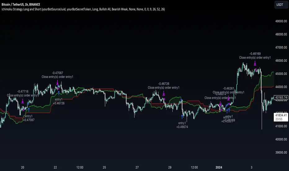
Ichimoku Clouds Strategy Long and ShortOverview:
The Ichimoku Clouds Strategy leverages the Ichimoku Kinko Hyo technique to offer traders a range of innovative features, enhancing market analysis and trading efficiency. This strategy is distinct in its combination of standard methodology and advanced customization, making it suitable for both novice and experienced traders.
Unique Features:
Enhanced Interpretation: The strategy introduces weak, neutral, and strong bullish/bearish signals, enabling detailed interpretation of the Ichimoku cloud and direct chart plotting.
Configurable Trading Periods: Users can tailor the strategy to specific market windows, adapting to different market conditions.
Dual Trading Modes: Long and Short modes are available, allowing alignment with market trends.
Flexible Risk Management: Offers three styles in each mode, combining fixed risk management with dynamic indicator states for versatile trade management.
Indicator Line Plotting: Enables plotting of Ichimoku indicator lines on the chart for visual decision-making support.
Methodology:
The strategy utilizes the standard Ichimoku Kinko Hyo model, interpreting indicator values with settings adjustable through a user-friendly menu. This approach is enhanced by TradingView's built-in strategy tester for customization and market selection.
Risk Management:
Our approach to risk management is dynamic and indicator-centric. With data from the last year, we focus on dynamic indicator states interpretations to mitigate manual setting causing human factor biases. Users still have the option to set a fixed stop loss and/or take profit per position using the corresponding parameters in settings, aligning with their risk tolerance.
Backtest Results:
Operating window: Date range of backtests is 2023.01.01 - 2024.01.04. It is chosen to let the strategy to close all opened positions.
Commission and Slippage: Includes a standard Binance commission of 0.1% and accounts for possible slippage over 5 ticks.
Maximum Single Position Loss: -6.29%
Maximum Single Profit: 22.32%
Net Profit: +10 901.95 USDT (+109.02%)
Total Trades: 119 (51.26% profitability)
Profit Factor: 1.775
Maximum Accumulated Loss: 4 185.37 USDT (-22.87%)
Average Profit per Trade: 91.67 USDT (+0.7%)
Average Trade Duration: 56 hours
These results are obtained with realistic parameters representing trading conditions observed at major exchanges such as Binance and with realistic trading portfolio usage parameters. Backtest is calculated using deep backtest option in TradingView built-in strategy tester
How to Use:
Add the script to favorites for easy access.
Apply to the desired chart and timeframe (optimal performance observed on the 1H chart, ForEx or cryptocurrency top-10 coins with quote asset USDT).
Configure settings using the dropdown choice list in the built-in menu.
Set up alerts to automate strategy positions through web hook with the text: {{strategy.order.alert_message}}
Disclaimer:
Educational and informational tool reflecting Skyrex commitment to informed trading. Past performance does not guarantee future results. Test strategies in a simulated environment before live implementation
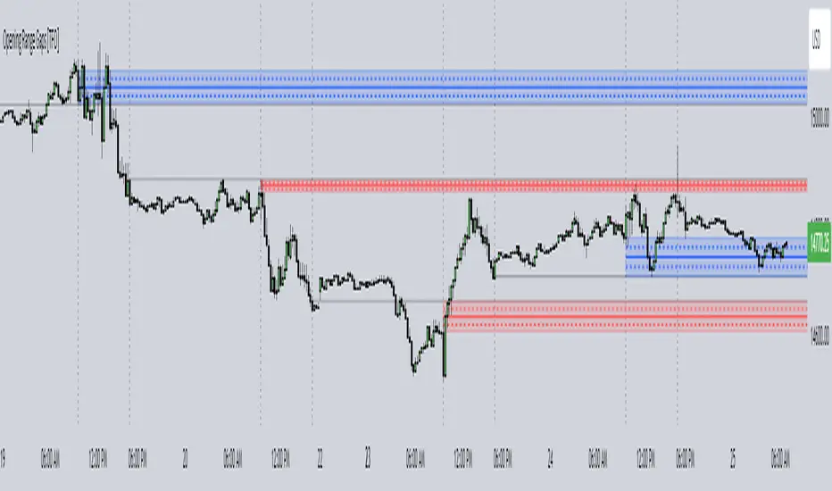
Opening Range Gaps [TFO]This indicator displays Opening Range Gaps with an adjustable time window. Its intention is to capture the discrepancy between the close price of previous and new Real Trading Hours (RTH) sessions, i.e. yesterday's close compared to today's open. A gap will be drawn from this area with a solid line denoting its midpoint, and dashed lines denoting the upper and lower quartiles of its range. Its color is determined by whether the new session open price is above or below the previous session close.
The Gap Session parameter allows users to define the specific time window for which to capture the "gap" in price. Using U.S. index futures as an example, we can use 16:00 - 09:30 (EST) to capture the discrepancy between the previous day's close price and the current day's open price. However, this parameter is left as adjustable for users that may want to observe different markets or simply experiment with different time windows.
Show Session Delineations will draw vertical timestamps denoting the start and end times of the provided Gap Session. Track Start Price serves as a visual aid to track the initial price of the Gap Session until its end price is validated, for easy visual verification of a gap's upper and lower bounds. With both options turned off, the indicator will only display the gap boxes and lines, as shown here:
Extend Boxes will draw all gaps with an indefinite extension to the right. This can get messy with a large number of boxes, which is why we have a Keep Last parameter to limit how many sessions' drawings should be stored. Any drawings that were made beyond this number of sessions in the past will automatically be deleted.
The Timeframe Limit will dictate that the indicator as a whole will only draw objects on timeframes less than or equal to this timeframe, determined by the user. In some cases this may help users avoid resolution errors which may arise from using timeframes that are too large for a given session. For example, if a user wanted to track a Gap Session of 16:15-09:30, the Timeframe Limit should be set to 15 minutes because the close price at 16:15 cannot be observed on a 30 minute chart (or greater).
Fibonacci ClustersI was reading about Fibonacci Clusters on investopedia (www.investopedia.com) and couldn't find a script for it on tradingveiw. Apparently some people use it successfully but I found it a little chaotic. This script will mark the retracements in a window's length, and you can set this for six windows. This script isn't very pretty because it doesn't seem obviously useful and pinescript has far too many deficiencies to fully flesh this idea out. I was able to make more sense out of larger windowing times (500-4000 periods), than shorter ones (25-333). Try it out, see what it shows you. Happy trading

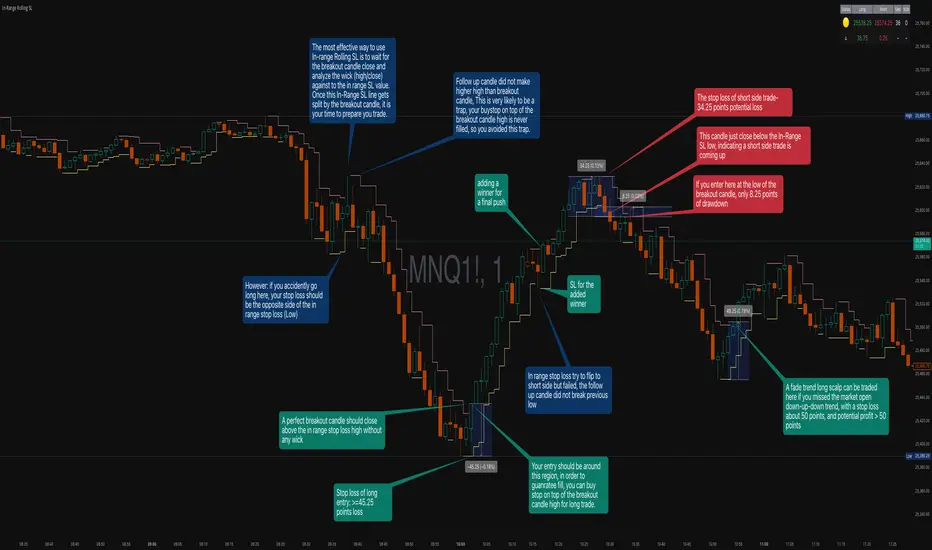
In-Range Rolling SL
In-Range Rolling SL Indicator Guide
The In-Range Rolling SL indicator is a dynamic stop-loss system designed for intraday trading that identifies squeeze conditions and trade entry opportunities based on rolling price windows.
Core Concept
The indicator analyzes the highest high and lowest low over a defined lookback period (default: 2 candles) to establish an "in-range" zone. When price stays within this range without breaking either boundary, it creates a squeeze condition—signaling potential breakout opportunities.
Trading Strategy
Wait for the Squeeze Setup
The most effective approach is to wait for the in-range stop-loss squeeze to form. This occurs when both the long SL (green line) and short SL (red line) are active simultaneously, indicated by the yellow status dot (🟡) in the indicator table. Analyze the wick high/close relationship against the in-range SL while price remains compressed—this setup identifies which side is more likely to break first.
Entry Timing and Risk Management
Long Entry: Enter when a candle closes above the in-range short SL (red line) without any wick above it. This "perfect breakout candle" confirms bullish momentum. Your entry should be around the region, with your stop-loss placed just below the top of the breakout candle's high.
Short Entry: Enter when a candle closes below the in-range long SL (green line). The stop-loss for short trades should be set 34.26 points above your entry for appropriate risk protection.
Risk-Reward Considerations
If you enter at the low of a breakout candle, expect only 8.26 points of drawdown potential. However, if you accidentally go long and your stop gets hit, you'll experience the full in-range stop-loss distance as your loss.
Advanced Techniques
Failed Breakout Trap: If a follow-up candle doesn't make a higher high after the initial breakout, consider adding a "winner" for compensation rather than holding for a trap. When your buy-stop sits on top of the breakout candle high, this isn't a valid long trade setup.
Flip Trade Opportunity: In-range stop-loss attempts to flip often provide ideal entry points. If the up candle doesn't break the previous low, this validates the long continuation.
Long Scalp Trading: A failed long scalp can be traded if you missed the initial market open down-up-down trend. With a stop-loss of 34 points and potential profit exceeding 50 points, this provides favorable risk-reward ratios.
Sustained Loss Management: Stop-loss for long positions should target 26 points maximum loss. The indicator automatically invalidates stop-losses when price violates them, keeping your chart clean for the next setup.
-------------------------
In-Range Rolling SL Indicator Guide
The In-Range Rolling SL indicator is a dynamic stop-loss system designed for intraday trading that identifies squeeze conditions and breakout opportunities based on rolling price windows.
How the Indicator Works
The indicator tracks the highest high and lowest low over your selected lookback period (default: 2 candles) to establish dynamic support and resistance levels. These levels create an "in-range" zone that adapts as new price action develops.
Visual Components
Green Line (Long SL): The rolling window's lowest low - your stop-loss level for long positions
Red Line (Short SL): The rolling window's highest high - your stop-loss level for short positions
Status Indicators:
🟡 Yellow: Squeeze condition (both SLs active)
🟢 Green: Long-only setup
🔴 Red: Short-only setup
⚪ White: Neutral (no active SLs)
The Squeeze Setup Strategy
Step 1: Wait for the Squeeze
The most effective way to use the In-Range Rolling SL is to wait for the in-range stop-loss squeeze to form. During the squeeze, both the green and red lines are active, meaning price has stayed within the rolling window without breaking either boundary. This compression phase indicates that it's "go time" to prepare your trade.
While in the squeeze, analyze the wick high/close relationship against the in-range SL levels. This analysis helps you determine which side is more likely to split when the breakout occurs.
Step 2: Identify the Perfect Breakout
Long Breakout: A perfect breakout candle should close above the in-range stop-loss high (red line) without any wick above it. This clean breakout demonstrates strong momentum and reduces the risk of a false breakout.
Short Breakout: Look for a candle that closes below the in-range SL low (green line), indicating a short-side trade is coming up.
Step 3: Entry Execution
Long Entry: Your entry should be around the region of the breakout. Position your stop-loss just below the top of the breakout candle's high. This placement protects you from failed breakouts while giving the trade room to develop.
Short Entry: Enter as the candle closes below the in-range SL low. The stop-loss for short-side trades is typically 34.26 points of potential loss based on the indicator's measurements.
Risk-Reward Analysis
Entry at Breakout Low
If you enter here at the low of the breakout candle, you're looking at only 8.26 points of drawdown potential. This represents your best-case entry scenario.
Accidental Wrong-Side Entry
However, if you accidentally go long here and your stop gets hit, you'll experience the full in-range stop-loss distance as your loss. This emphasizes the importance of waiting for clear breakout confirmation.
Long Scalp Opportunity
A failed long scalp can be traded here if you missed the market open down-up-down trend. With a stop-loss of 34 points and potential profit greater than 50 points, this setup offers a favorable risk-reward ratio of approximately 1:1.5.
Advanced Trade Management
Failed Breakout Recognition
Follow-Up Candle Validation: If a follow-up candle did not make a higher high than the breakout candle, this could be a trap. Your buy-stop on top of the breakout candle high is not a valid long trade setup in this scenario. Consider adding a "winner" for compensation rather than holding through the potential reversal.
Flip Trade Opportunities
In-range stop-loss tries to flip to the other side often provide excellent entries. If the up candle did not break the previous low, this validates the long continuation and suggests the squeeze is resolving to the upside.
Sustained Position Management
Stop-Loss Guidelines: Stop-loss for long positions should be 26 points of maximum loss. The indicator table displays the delta (Δ) showing your real-time distance to the active stop-loss, helping you manage risk dynamically.
Entry Timing: Your entry should be around the region where the breakout confirms, rather than chasing price after a large move. In order to prepare your trade, position your stop-loss on top of the breakout candle's high for long trades.
Practical Example from the Chart
Looking at the MNQ1! chart, you can see multiple squeeze formations throughout the session. The most notable sequence shows:
An initial downtrend creating a squeeze setup
A perfect breakout candle closing above the red line without upper wick
The subsequent candle validating the move
Later, a failed breakout attempt that created a short opportunity
Multiple flip attempts that provided re-entry points for scalpers
The indicator's table in the top-right continuously updates with the current SL levels, gap size, candle size, and delta values - giving you all the information needed to assess each trade's risk-reward profile in real-time.
Dual Harmonic-based AHR DCA (Default :BTC-ETH)A panel indicator designed for dual-asset BTC/ETH DCA (Dollar Cost Averaging) decisions.
It is inspired by the Chinese community indicator "AHR999" proposed by “Jiushen”.
How to use:
Lower HM-based AHR → cheaper (potential buy zone).
Higher HM-based AHR → more expensive (potential risk zone).
Higher than Risk Threshold → consider to sell, but not suitable for DCA.
When both AHR lines are below the Risk threshold → buy the cheaper one (or split if similar).
If one AHR is above Risk → buy the other asset.
If both are above Risk → simulation shows “STOP (both risk)”.
Not limited to BTC/ETH — you can freely change symbols in the input panel
to build any dual-asset DCA pair you want (e.g., BTC/BNB, ETH/SOL, etc.).
What you’ll see:
Two lines: AHR BTC (HM) and AHR ETH (HM)
Two dashed lines: OppThreshold (green) and RiskThreshold (red)
Colored fill showing which asset is cheaper (BTC or ETH)
Buy markers:
- B = Buy BTC
- E = Buy ETH
- D = Dual (split budget)
Top-right table: prices, AHRs, thresholds, qOpp/qRisk%, simulation, P&L
Labels showing last-bar AHR values
Core idea:
Use an AHR based on Harmonic Moving Average (HM) — a ratio that measures how “cheap or expensive” price is relative to both its short-term mean and long-term trend.
The original AHR999 used SMA and was designed for BTC only.
This indicator extends it with cross-exchange percentile mapping, allowing the empirical “opportunity/risk” zones of the AHR999 (on Bitstamp) to adapt automatically to the current market pair.
The indicator derives two adaptive thresholds:
OppThreshold – opportunity zone
RiskThreshold – risk zone
These thresholds are compared with the current HM-based AHR of BTC and ETH to decide which asset is cheaper, and whether it is good to DCA or not, or considering to sell(When it in risk area).
This version uses
Display base: Binance (default: perpetual) with HM-based AHR
Percentile base: Bitstamp spot SMA-AHR (complete, stable history)
Rolling window: 2920 daily bars (~8 years) for percentile tracking
Concept summary
AHR measures the ratio of price to its long-term regression and short-term mean.
HM replaces SMA to better reflect equal-fiat-cost DCA behavior.
Cross-exchange percentile mapping (Bitstamp → Binance) keeps thresholds consistent with the original AHR999 interpretation.
Recommended settings (1D):
DCA length (harmonic): 200
Log-regression lookback: 1825 (≈5 years)
Rolling window: 2920 (≈8 years)
Reference thresholds: 0.45 / 1.20 (AHR999 empirical priors)
Tie split tolerance (ΔAHR): 0.05
Daily budget: 15 USDT (simulation)
All display options can be toggled: table, markers, labels, etc.
Notes:
When the rolling window is filled (2920 bars by default), thresholds are first calculated and then visually backfilled as left-extended lines.
The “buy markers” and “decision table” are light simulations without fees or funding costs — for rhythm and relative analysis, not backtesting.

Sunmool's NY Lunch Model BacktestingICT NY Lunch Model Backtesting (12:00–13:00 NY) 🗽🍔
This research indicator tests an ICT narrative using the New York lunch window (12:00–13:00 America/New_York). It records that hour’s high/low and measures, during the post-lunch session (default 13:00–16:00), how often:
⬆️ If the afternoon trends up, the Lunch Low gets swept first.
⬇️ If the afternoon trends down, the Lunch High gets swept first.
It reports these as conditional probabilities, not trade signals. 📈
👀 What it shows
🟦 Lunch Range box (toggle): high/low from 12:00–13:00 NY
🔻🔺 Sweep signals (bar-anchored)
Low sweep: triangle below bar + optional “L”
High sweep: triangle above bar + optional “H”
🧱 Optional small box wrapping the swept candle
📊 Stats table (top-right)
P(L-swept | Up) — % of Up-days where Lunch Low was swept
P(H-swept | Down) — % of Down-days where Lunch High was swept
🔁 Contradictions + sample sizes (Up-days / Down-days)
🎯 Direction logic (Up/Down)
Anchor: 13:00 open (pmOpen) ⏰
Threshold: ATR × multiple or % from 13:00
Close ≥ pmOpen + threshold → Up-day
Close ≤ pmOpen − threshold → Down-day
Tiny moves under the threshold are ignored to reduce noise 🧹
⚙️ Inputs
🌐 Timezone: America/New_York (DST handled)
🍽️ Lunch window: 1200–1300
🕓 Post-lunch window: default 1300–1600 (try 17:00/20:00 for sensitivity)
📐 Trend threshold: ATR / Percent (with length/multiple or % level)
📅 Weekdays-only toggle (FX/Equities style)
👁️ Display toggles: Lunch box / sweep arrows / sweep text / sweep candle box / stats table
🔔 TF hint when chart TF > 15m
🧭 How to use
Use 5–15m charts for accurate lunch range capture.
Scroll ~1 year for meaningful samples.
Run sensitivity checks: vary ATR/% thresholds and the post-lunch end time.
For crypto, compare with vs without weekends. 🚀
🧠 Reading the results
High P(L-swept | Up) with a solid Up-day count ⇒ on up afternoons, lunch low is often swept.
High P(H-swept | Down) ⇒ on down afternoons, lunch high is often swept.
Lower Contradictions = cleaner tendency.
Remember: this is a probabilistic tendency, not a rule. 🎲
📝 Notes & limits
All markers (arrows, text, sweep boxes) are bar-anchored; the lunch range box is a research overlay you can toggle.
Real-time vs historical bar building can differ—interpret on bar close. 🔒

Theil-Sen Line Filter [BackQuant]Theil-Sen Line Filter
A robust, median-slope baseline that tracks price while resisting outliers. Designed for the chart pane as a clean, adaptive reference line with optional candle coloring and slope-flip alerts.
What this is
A trend filter that estimates the underlying slope of price using a Theil-Sen style median of past slopes, then advances a baseline by a controlled fraction of that slope each bar. The result is a smooth line that reacts to real directional change while staying calm through noise, gaps, and single-bar shocks.
Why Theil-Sen
Classical moving averages are sensitive to outliers and shape changes. Ordinary least squares is sensitive to large residuals. The Theil-Sen idea replaces a single fragile estimate with the median of many simple slopes, which is statistically robust and less influenced by a few extreme bars. That makes the baseline steadier in choppy conditions and cleaner around regime turns.
What it plots
Filtered baseline that advances by a fraction of the robust slope each bar.
Optional candle coloring by baseline slope sign for quick trend read.
Alerts when the baseline slope turns up or down.
How it behaves (high level)
Looks back over a fixed window and forms many “current vs past” bar-to-bar slopes.
Takes the median of those slopes to get a robust estimate for the bar.
Optionally caps the magnitude of that per-bar slope so a single volatile bar cannot yank the line.
Moves the baseline forward by a user-controlled fraction of the estimated slope. Lower fractions are smoother. Higher fractions are more responsive.
Inputs and what they do
Price Source — the series the filter tracks. Typical is close; HL2 or HLC3 can be smoother.
Window Length — how many bars to consider for slopes. Larger windows are steadier and slower. Smaller windows are quicker and noisier.
Response — fraction of the estimated slope applied each bar. 1.00 follows the robust slope closely; values below 1.00 dampen moves.
Slope Cap Mode — optional guardrail on each bar’s slope:
None — no cap.
ATR — cap scales with recent true range.
Percent — cap scales with price level.
Points — fixed absolute cap in price points.
ATR Length / Mult, Cap Percent, Cap Points — tune the chosen cap mode’s size.
UI Settings — show or hide the line, paint candles by slope, choose long and short colors.
How to read it
Up-slope baseline and green candles indicate a rising robust trend. Pullbacks that do not flip the slope often resolve in trend direction.
Down-slope baseline and red candles indicate a falling robust trend. Bounces against the slope are lower-probability until proven otherwise.
Flat or frequent flips suggest a range. Increase window length or decrease response if you want fewer whipsaws in sideways markets.
Use cases
Bias filter — only take longs when slope is up, shorts when slope is down. It is a simple way to gate faster setups.
Stop or trail reference — use the line as a trailing guide. If price closes beyond the line and the slope flips, consider reducing exposure.
Regime detector — widen the window on higher timeframes to define major up vs down regimes for asset rotation or risk toggles.
Noise control — enable a cap mode in very volatile symbols to retain the line’s continuity through event bars.
Tuning guidance
Quick swing trading — shorter window, higher response, optionally add a percent cap to keep it stable on large moves.
Position trading — longer window, moderate response. ATR cap tends to scale well across cycles.
Low-liquidity or gappy charts — prefer longer window and a points or ATR cap. That reduces jumpiness around discontinuities.
Alerts included
Theil-Sen Up Slope — baseline’s one-bar change crosses above zero.
Theil-Sen Down Slope — baseline’s one-bar change crosses below zero.
Strengths
Robust to outliers through median-based slope estimation.
Continuously advances with price rather than re-anchoring, which reduces lag at turns.
User-selectable slope caps to tame shock bars without over-smoothing everything.
Minimal visuals with optional candle painting for fast regime recognition.
Notes
This is a filter, not a trading system. It does not account for execution, spreads, or gaps. Pair it with entry logic, risk management, and higher-timeframe context if you plan to use it for decisions.

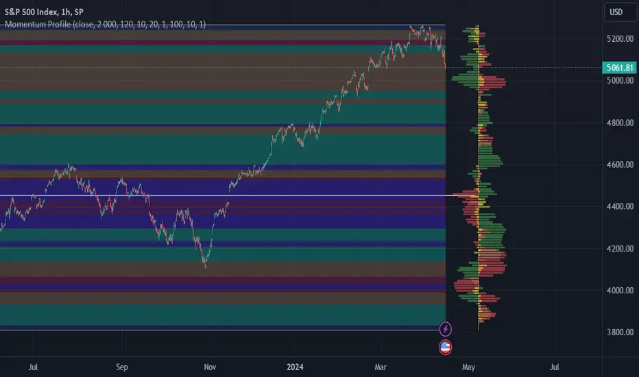
Momentum ProfileProfile market behavior in horizontal zones
Profile Sidebar
Buckets pointing rightward indicate upward security movement in the lookahead window at that level, and buckets pointing leftward indicate downward movement in the lookahead window.
Green profile buckets indicate the security's behavior following an uptrend in the lookbehind window. Conversely, Red profile buckets show security's behavior following a downtrend in the lookbehind window. Yellow profile buckets show behavior following sideways movement.
Buckets length corelates with the amount of movement measured in that direction at that level.
Inputs
Length determines how many bars back are considered for the calculation. On most securities, this can be increased to just above 4000 without issues.
Rows determines the number of buckets that the securities range is divided into.
You can increase or decrease the threshold for which moves are considered sideways with the sideways_filter input: higher means more moves are considered sideways.
The lookbehind input determines the lookbehind window. Specifically, how many bars back are considered when determining whether a data point is considered green (uptrend), red (downtrend), or yellow (no significant trend).
The lookahead input determines how many bars after the current bar are considered when determining the length and direction of each bucket (leftward for downward moves, rightward for upward moves).
Profile_width and Profile_spacing are cosmetic choices.
Intrabar support is not current supported.
Region Highlighting
Regions highlighted green saw an upward move in the lookahead window for both lookbehind downtrends and uptrends. In other words, both red and green profile buckets pointed rightward.
Regions highlighted red saw a downward move in the lookahead window both for lookbehind downtrends and uptrends.
Regions highlighted brown indicate a reversal region: uptrends were followed by downtrends, and vice versa. These regions often indicate a chop range or sometimes support/resistance levels. On the profile, this means that green buckets pointed left, and red buckets pointed right.
Regions highlighted purple indicate that whatever direction the security was moving, it continued that way. On the profile, this means that green buckets pointed right, and red buckets pointed left in that region.
Volume Forecasting [LuxAlgo]The Volume Forecasting indicator provides a forecast of volume by capturing and extrapolating periodic fluctuations. Historical forecasts are also provided to compare the method against volume at time t .
This script will not work on tickers that do not have volume data.
🔶 SETTINGS
Median Memory: Number of days used to compute the median and first/third quartiles.
Forecast Window: Number of bars forecasted in the future.
Auto Forecast Window: Set the forecast window so that the forecast length completes an interval.
🔶 USAGE
The periodic nature of volume on certain securities allows users to more easily forecast using historical volume. The forecast can highlight intervals where volume tends to be more important, that is where most trading activity takes place.
More pronounced periodicity will tend to return more accurate forecasts.
The historical forecast can also highlight intervals where high/low volume is not expected.
The interquartile range is also highlighted, giving an area where we can expect the volume to lie.
🔶 DETAILS
This forecasting method is similar to the time series decomposition method used to obtain the seasonal component.
We first segment the chart over equidistant intervals. Each interval is delimited by a change in the daily timeframe.
To forecast volume at time t+1 we see where the current bar lies in the interval, if the bar is the 78th in interval then the forecast on the next bar is made by taking the median of the 79th bar over N intervals, where N is the median memory.
This method ensures capturing the periodic fluctuation of volume.

Bill Williams SystemBill Williams System combine all indicators of Mr. Bill Williams into one window with detail below:
1. Top of window:
Display Fractals with shape triangle down is bottom fractal and shape triangle up is top fractal
2. Bottom of window:
Display Alligator Trend Flat with trend defined as below:
* Up trend: Lips value shift 3 bars greater than Teeth value shift 5 bars. And Teeth value shift 5 bars greater than Jaws value shift 8 bars. By default up trend is green square.
* Down trend: Lips value shift 3 bars less than Teeth value shift 5 bars. And Teeth value shift 5 bars less than Jaws value shift 8 bars. By default down trend is red square.
* Choppy: not up trend and not down trend. By default choppy is gray square.
3. Moving around zero line
* Awesome Oscillator is circles.
* Accelerator Oscillator is columns.
* Gator Oscillator is area.

Session Dynamics & Pivot Overlay (Arjo)## **OVERVIEW**
The **Session Dynamics & Pivot Overlay (Arjo)** is a visual analysis tool that displays session-based price ranges, anchored volume-weighted averages, daily pivot levels, and smoothed trend conditions on the chart. It highlights how price interacts with custom sessions, midpoint levels, and dynamic ranges, providing a structured visual layout that helps users observe market behavior over time without implying any form of prediction or trading signal.
## **CONCEPTS**
This indicator incorporates several widely used analytical concepts:
- **Session Ranges:** Identifies user-defined time windows and visually displays their high, low, and midpoint behavior throughout the session.
- **VWAP (Morning Session):** Shows volume-weighted average price calculations for a defined morning period, assisting with visual comparison between price and weighted averages.
- **Daily Pivot Levels:** Displays R1–R2, S1–S2, central pivot, and associated levels derived from prior daily price data.
- **Trend Smoothing:** Uses SuperSmoother filtering and an additional EMA to highlight whether the smoothed trend is rising or falling.
- **EMA + ATR Bands:** Plots a 20-period EMA with upper and lower ATR-derived bands to help visualize short-term price displacement relative to average true range.
All of these elements are presented solely for structural and comparative chart analysis.
## **FEATURES**
- **Custom Session Visualization:** Automatically draws session boxes, capturing the evolving high, low, and midpoint throughout the defined intraday window.
- **Dynamic Midline Calculation:** A midpoint line is updated continuously during the session to visually anchor price within the session’s range.
- **Morning Session VWAP:** Displays a dedicated VWAP line for the morning window with adjustable source and configuration options.
- **Daily Pivot Lines:** Automatically plots pivot, BC/TC, R1–R2, and S1–S2 levels with customizable colors, widths, and line styles.
- **Trend-Responsive Pivot Display:** Optionally toggles visibility of R2 or S2 depending on the direction of the smoothed trend.
- **EMA + ATR Zones:** Renders a 20-EMA and ATR-based support/resistance zone using filled regions for enhanced visual clarity.
- **Full Customization:** Multiple color, transparency, line-style, and display options allow users to adapt the presentation to their charting preferences.
- **Overlay Compatible:** Designed to work directly on price charts without obstructing candles or other overlays.
## **HOW TO USE**
Users can interact with the indicator entirely through the settings panel:
- Adjust session timings to match preferred market hours or custom internal zones.
- Enable or disable the display of pivot levels, VWAP, or the ATR/EMA zone.
- Customize colors and line styles to improve visibility according to the chart background or personal preference.
- Observe how price behaves relative to the session box, midpoint, VWAP, and pivot levels for contextual understanding.
- Utilize the smoothed trend condition to see when the indicator chooses to display certain pivot extensions.
These elements help users interpret chart structure, volatility, and intraday behavior in a visually organized manner.
## **CONCLUSION**
The ** Session Dynamics & Pivot Overlay (Arjo) ** indicator offers a consolidated view of session structure, pivot levels, VWAP, and smoothed trend conditions. Its purpose is to improve visual clarity and assist users in understanding market context without issuing directives or trade suggestions. It functions as an educational tool that enhances chart interpretation and supports structured analysis.
---
## **DISCLAIMER**
This indicator is for educational and visual analysis purposes only. It does not provide trading signals, financial advice, or guaranteed outcomes. Users should conduct their own research and consult a licensed financial professional when necessary. All trading decisions are solely the responsibility of the user.
Happy Trading (Arjo)

PoC Migration Map [BackQuant]PoC Migration Map
A volume structure tool that builds a side volume profile, extracts rolling Points of Control (PoCs), and maps how those PoCs migrate through time so you can see where value is moving, how volume clusters shift, and how that aligns with trend regime.
What this is
This indicator combines a classic volume profile with a segmented PoC trail. It looks back over a configurable window, splits that window into bins by price, and shows you where volume has concentrated. On top of that, it slices the lookback into fixed bar segments, finds the local PoC in each segment, and plots those PoCs as a chain of nodes across the chart.
The result is a "migration map" of value:
A side volume profile that shows how volume is distributed over the recent price range.
A sequence of PoC nodes that show where local value has been accepted over time.
Lines that connect those PoCs to reveal the path of value migration.
Optional trend coloring based on EMA 12 and EMA 21, so each PoC also encodes trend regime.
Used together, this gives you a structural read on where the market has actually traded size, how "value" is moving, and whether that movement is aligned or fighting the current trend.
Core components
Lookback volume profile - a side histogram built from all closes and volumes in the chosen lookback window.
Segmented PoC trail - rolling PoCs computed over fixed bar segments, plotted as nodes in time.
Trend heatmap - optional color mapping of PoC nodes using EMA 12 versus EMA 21.
PoC labels - optional labels on every Nth PoC for easier reading and referencing.
How it works
1) Global lookback and binning
You choose:
Lookback Bars - how far back to collect data.
Number of Bins - how finely to split the price range.
The script:
Finds the highest high and lowest low in the lookback.
Computes the total price range and divides it into equal binCount slices.
Assigns each bar's close and volume into the appropriate price bin.
This creates a discretized volume distribution across the entire lookback.
2) Side volume profile
If "Show Side Profile" is enabled, a right-hand volume profile is drawn:
Each bin becomes a horizontal bar anchored at a configurable "Right Offset" from the current bar.
The horizontal width of each bar is proportional to that bin's volume relative to the maximum volume bin.
Optionally, volume values and percentages are printed inside the profile bars.
Color and transparency are controlled by:
Base Profile Color and its transparency.
A gradient that uses relative volume to modulate opacity between lower volume and higher volume bins.
Profile Width (%) - how wide the maximum bin can extend in bars.
This gives you an at-a-glance view of the volume landscape for the chosen lookback window.
3) Segmenting for PoC migration
To build the PoC trail, the lookback is divided into segments:
Bars per Segment - bars in each local cluster.
Number of Segments - how many segments you want to see back in time.
For each segment:
The script uses the same price bins and accumulates volume only from bars in that segment.
It finds the bin with the highest volume in that segment, which is the local PoC for that segment.
It sets the PoC price to the center of that bin.
It finds the "mid bar" of the segment and places the PoC node at that time on the chart.
This is repeated for each segment from older to newer, so you get a chain of PoCs that shows how local value has migrated over time.
4) Trend regime and color coding
The indicator precomputes:
EMA 12 (Fast).
EMA 21 (Slow).
For each PoC:
It samples EMA 12 and EMA 21 at the mid bar of that segment.
It computes a simple trend score as fast EMA minus slow EMA.
If trend heatmap is enabled, PoC nodes (and the lines between them) are colored by:
Trend Up Color if EMA 12 is above EMA 21.
Trend Down Color if EMA 12 is below EMA 21.
Trend Flat Color if they are roughly equal.
If the trend heatmap is disabled, PoC color is instead based on PoC migration:
If the current PoC is above the previous PoC, use the Up PoC Color.
If the current PoC is below the previous PoC, use the Down PoC Color.
If unchanged, use the Flat PoC Color.
5) Connecting PoCs and labels
Once PoC prices and times are known:
Each PoC is connected to the previous one with a dotted line, using the PoC's color.
Optional labels are placed next to every Nth PoC:
Label text uses a simple "PoC N" scheme.
Label background uses a configurable label background color.
Label border is colored by the PoC's own color for visual consistency.
This turns the PoCs into a visual path that can be read like a "value trajectory" across the chart.
What it plots
When fully enabled, you will see:
A right-sided volume profile for the chosen lookback window, built from volume by price.
Colored horizontal bars representing each price bin's relative volume.
Optional volume text showing each bin's volume and its percentage of the profile maximum.
A series of PoC nodes spaced across the chart at the mid point of each segment.
Dotted lines connecting those PoCs to show the migration path of value.
Optional PoC labels at each Nth node for easier reference.
Color-coding of PoCs and lines either by EMA 12 / 21 trend regime or by up/down PoC drift.
Reading PoC migration and market pressure
Side profile as a pressure map
The side profile shows where trading has been most active:
Thick, opaque bars represent high volume zones and possible high interest or acceptance areas.
Thin, faint bars represent low volume zones, potential rejection or transition areas.
When price trades near a high volume bin, the market is sitting on an area of prior acceptance and size.
When price moves quickly through low volume bins, it often does so with less friction.
This gives you a static map of where the market has been willing to do business within your lookback.
PoC trail as a value migration map
The PoC chain represents "where value has lived" over time:
An upward sloping PoC trail indicates value migrating higher. Buyers have been willing to transact at increasingly higher prices.
A downward sloping trail indicates value migrating lower and sellers pushing the center of mass down.
A flat or oscillating trail indicates balance or rotational behaviour, with no clear directional acceptance.
Taken together, you can interpret:
Side profile as "where the volume mass sits", a static pressure field.
PoC trail as "how that mass has moved", the dynamic path of value.
Trend heatmap as a regime overlay
When PoCs are colored by the EMA 12 / 21 spread:
Green PoCs mark segments where the faster EMA is above the slower EMA, that is, a local uptrend regime.
Red PoCs mark segments where the faster EMA is below the slower EMA, that is, a local downtrend regime.
Gray PoCs mark flat or ambiguous trend segments.
This lets you answer questions like:
"Is value migrating higher while the trend regime is also up?" (trend confirming value).
"Is value migrating higher but most PoCs are red?" (value against the prevailing trend).
"Has value started to roll over just as PoCs flip from green to red?" (early regime transition).
Key settings
General Settings
Lookback Bars - how many bars back to use for both the global volume profile and segment profiles.
Number of Bins - how many price bins to split the high to low range into.
Profile Settings
Show Side Profile - toggle the right-hand volume profile on or off.
Profile Width (%) - how wide the largest volume bar is allowed to be in terms of bars.
Base Profile Color - the starting color for profile bars, with transparency.
Show Volume Values - if enabled, print volume and percent for each non-zero bin.
Profile Text Color - color for volume text inside the profile.
PoC Migration Settings
Show PoC Migration - toggle the PoC trail plotting.
Bars per Segment - the number of bars contained in each segment.
Number of Segments - how many segments to build backwards from the current bar.
Horizontal Spacing (bars) - spacing between PoC nodes when drawn. (Used to separate PoCs horizontally.)
Label Every Nth PoC - draw labels at every Nth PoC (0 or 1 to suppress labels).
Right Offset (bars) - horizontal offset to anchor the side profile on the right.
Up PoC Color - color used when a PoC is higher than the previous one, if trend heatmap is off.
Down PoC Color - color used when a PoC is lower than the previous one, if trend heatmap is off.
Flat PoC Color - color used when the PoC is unchanged, if trend heatmap is off.
PoC Label Background - background color for PoC labels.
Trend Heatmap Settings
Color PoCs By Trend (EMA 12 / 21) - when enabled, overrides simple up/down coloring and uses EMA-based trend colors.
Fast EMA - length for the fast EMA.
Slow EMA - length for the slow EMA.
Trend Up Color - color for PoCs in a bullish EMA regime.
Trend Down Color - color for PoCs in a bearish EMA regime.
Trend Flat Color - color for neutral or flat EMA regimes.
Trading applications
1) Value migration and trend confirmation
Use the PoC path to see if value is following price or lagging it:
In a healthy uptrend, price, PoCs, and trend regime should all lean higher.
In a weakening trend, price may still move up, but PoCs flatten or start drifting lower, suggesting fewer participants are accepting the new highs.
In a downtrend, persistent downward PoC migration confirms that sellers are winning the value battle.
2) Identifying acceptance and rejection zones
Combine the side profile with PoC locations:
High volume bins near clustered PoCs mark strong acceptance zones, good areas to watch for re-tests and decision points.
PoCs that quickly jump across low volume areas can indicate rejection and fast repricing between value zones.
High volume zones with mixed PoC colors may signal balance or prolonged negotiation.
3) Structuring entries and exits
Use the map to refine trade location:
Fade trades against value migration are higher risk unless you see clear signs of exhaustion or regime change.
Pullbacks into prior PoC zones in the direction of the current PoC slope can offer higher quality entries.
Stops placed beyond major accepted zones (clusters of PoCs and high volume bins) are less likely to be hit by random noise.
4) Regime transitions
Watch how PoCs behave as the EMA regime changes:
A flip in EMA 12 versus EMA 21, coupled with a turn in PoC slope, is a strong signal that value is beginning to move with the new trend.
If EMAs flip but PoC migration does not follow, the trend signal may be early or false.
A weakening PoC path (lower highs in PoCs) while trend colors are still green can warn of a late-stage trend.
Best practices
Start with a moderate lookback such as 200 to 300 bars and a moderate bin count such as 20 to 40. Too many bins can make the profile overly granular and sparse.
Align "Bars per Segment" with your trading horizon. For example, 5 to 10 bars for intraday, 10 to 20 bars for swing.
Use the profile and PoC trail as structural context rather than as a direct buy or sell signal. Combine with your existing setups for timing.
Pay attention to clusters of PoCs at similar prices. Those are areas where the market has repeatedly accepted value, and they often matter on future tests.
Notes
This is a structural volume tool, not a complete trading system. It does not manage execution, position sizing or risk management. Use it to understand:
Where the bulk of trading has occurred in your chosen window.
How the center of volume has migrated over time.
Whether that migration is aligned with or fighting the current trend regime.
By turning PoC evolution into a visible path and adding a trend-aware heatmap, the PoC Migration Map makes it easier to see how value has been moving, where the market is likely to feel "heavy" or "light", and how that structure fits into your trading decisions.

Regime MapRegime Map — Volatility State Detector
This indicator is a PineScript friendly approximation of a more advanced Python regime-analysis engine.
The original backed identifies market regimes using structural break detection, Hidden-Markov Models, wavelet decomposition, and long-horizon volatility clustering. Since Pine Script cannot execute these statistical models directly, this version implements a lightweight, real-time proxy using realised volatility and statistical thresholds.
The purpose is to provide a clear visual map of evolving volatility conditions without requiring any heavy offline computation.
________________________________________
Mathematical Basis: Python vs Pine
1. Volatility Estimation
Python (Realised Volatility):
RVₜ = √N × stdev( log(Pₜ) − log(Pₜ₋₁) )
Pine Approximation:
RVₜ = stdev( log(Pₜ) − log(Pₜ₋₁), lookback )
Rationale:
Realised volatility captures volatility clustering — a key characteristic of regime transitions.
________________________________________
2. Regime Classification
Python (HMM Volatility States):
Volatility is modelled as belonging to hidden states with different means and variances:
State μ₁, σ₁
State μ₂, σ₂
State μ₃, σ₃
with state transitions determined by a probability matrix.
Pine Approximation (Z-Score Regimes):
Zₜ = ( RVₜ − mean(RV) ) / stdev(RV)
Regime assignment:
• Regime 0 (Low Vol): Zₜ < Zₗₒw
• Regime 1 (Normal): Zₗₒw ≤ Zₜ ≤ Zₕᵢgh
• Regime 2 (High Vol): Zₜ > Zₕᵢgh
Rationale:
Z-scores provide clean statistical boundaries that behave similarly to HMM state separation but are computable in real time.
________________________________________
3. Structural Break Detection vs Rolling Windows
Python (Bai–Perron Structural Breaks):
Segments the volatility series into periods with distinct statistical properties by minimising squared error over multiple regimes.
Pine Approximation:
Rolling mean and rolling standard deviation of volatility over a long window.
Rationale:
When structural breaks are not available, long-window smoothing approximates slow regime changes effectively.
________________________________________
4. Multi-Scale Cycles
Python (Wavelet Decomposition):
Volatility decomposed into long-cycle (A₄) and short-cycle components (D bands).
Pine Approximation:
Single-scale smoothing using long-horizon averages of RV.
Rationale:
Wavelets reveal multi-frequency behaviour; Pine captures the dominant low-frequency component.
________________________________________
Indicator Output
The background colour reflects the active volatility regime:
• Low Volatility (Green): trending behaviour, cleaner directional movement
• Normal Volatility (Yellow): balanced environment
• High Volatility (Red): sharp swings, traps, mean-reversion phases
Regime labels appear on the chart, with a status panel displaying the current regime.
________________________________________
Operational Logic
1. Compute log returns
2. Calculate short-horizon realised volatility
3. Compute long-horizon mean and standard deviation
4. Derive volatility Z-score
5. Assign regime classification
6. Update background colour and labels
This provides a stable, real-time map of market state transitions.
________________________________________
Practical Applications
Intraday Trading
• Low-volatility regimes favour trend and breakout continuation
• High-volatility regimes favour mean reversion and wide stop placement
Swing Trading
• Compression phases often precede multi-day trending moves
• Volatility expansions accompany distribution or panic events
Risk Management
• Enables volatility-adjusted position sizing
• Helps avoid leverage during expansion regimes
________________________________________
Notes
• Does not repaint
• Fully configurable thresholds and lookbacks
• Works across indices, stocks, FX, crypto
• Designed for real-time volatility regime identification
________________________________________
Disclaimer
This script is intended solely for educational and research purposes.
It does not constitute financial advice or a recommendation to buy or sell any instrument.
Trading involves risk, and past volatility patterns do not guarantee future outcomes.
Users are responsible for their own trading decisions, and the author assumes no liability for financial loss.

Range Oscillator Strategy + Stoch Confirm🔹 Short summary
This is a free, educational long-only strategy built on top of the public “Range Oscillator” by Zeiierman (used under CC BY-NC-SA 4.0), combined with a Stochastic timing filter, an EMA-based exit filter and an optional risk-management layer (SL/TP and R-multiple exits). It is NOT financial advice and it is NOT a magic money machine. It’s a structured framework to study how range-expansion + momentum + trend slope can be combined into one rule-based system, often with intentionally RARE trades.
────────────────────────
0. Legal / risk disclaimer
────────────────────────
• This script is FREE and public. I do not charge any fee for it.
• It is for EDUCATIONAL PURPOSES ONLY.
• It is NOT financial advice and does NOT guarantee profits.
• Backtest results can be very different from live results.
• Markets change over time; past performance is NOT indicative of future performance.
• You are fully responsible for your own trades and risk.
Please DO NOT use this script with money you cannot afford to lose. Always start in a demo / paper trading environment and make sure you understand what the logic does before you risk any capital.
────────────────────────
1. About default settings and risk (very important)
────────────────────────
The script is configured with the following defaults in the `strategy()` declaration:
• `initial_capital = 10000`
→ This is only an EXAMPLE account size.
• `default_qty_type = strategy.percent_of_equity`
• `default_qty_value = 100`
→ This means 100% of equity per trade in the default properties.
→ This is AGGRESSIVE and should be treated as a STRESS TEST of the logic, not as a realistic way to trade.
TradingView’s House Rules recommend risking only a small part of equity per trade (often 1–2%, max 5–10% in most cases). To align with these recommendations and to get more realistic backtest results, I STRONGLY RECOMMEND you to:
1. Open **Strategy Settings → Properties**.
2. Set:
• Order size: **Percent of equity**
• Order size (percent): e.g. **1–2%** per trade
3. Make sure **commission** and **slippage** match your own broker conditions.
• By default this script uses `commission_value = 0.1` (0.1%) and `slippage = 3`, which are reasonable example values for many crypto markets.
If you choose to run the strategy with 100% of equity per trade, please treat it ONLY as a stress-test of the logic. It is NOT a sustainable risk model for live trading.
────────────────────────
2. What this strategy tries to do (conceptual overview)
────────────────────────
This is a LONG-ONLY strategy designed to explore the combination of:
1. **Range Oscillator (Zeiierman-based)**
- Measures how far price has moved away from an adaptive mean.
- Uses an ATR-based range to normalize deviation.
- High positive oscillator values indicate strong price expansion away from the mean in a bullish direction.
2. **Stochastic as a timing filter**
- A classic Stochastic (%K and %D) is used.
- The logic requires %K to be below a user-defined level and then crossing above %D.
- This is intended to catch moments when momentum turns up again, rather than chasing every extreme.
3. **EMA Exit Filter (trend slope)**
- An EMA with configurable length (default 70) is calculated.
- The slope of the EMA is monitored: when the slope turns negative while in a long position, and the filter is enabled, it triggers an exit condition.
- This acts as a trend-protection exit: if the medium-term trend starts to weaken, the strategy exits even if the oscillator has not yet fully reverted.
4. **Optional risk-management layer**
- Percentage-based Stop Loss and Take Profit (SL/TP).
- Risk/Reward (R-multiple) exit based on the distance from entry to SL.
- Implemented as OCO orders that work *on top* of the logical exits.
The goal is not to create a “holy grail” system but to serve as a transparent, configurable framework for studying how these concepts behave together on different markets and timeframes.
────────────────────────
3. Components and how they work together
────────────────────────
(1) Range Oscillator (based on “Range Oscillator (Zeiierman)”)
• The script computes a weighted mean price and then measures how far price deviates from that mean.
• Deviation is normalized by an ATR-based range and expressed as an oscillator.
• When the oscillator is above the **entry threshold** (default 100), it signals a strong move away from the mean in the bullish direction.
• When it later drops below the **exit threshold** (default 30), it can trigger an exit (if enabled).
(2) Stochastic confirmation
• Classic Stochastic (%K and %D) is calculated.
• An entry requires:
- %K to be below a user-defined “Cross Level”, and
- then %K to cross above %D.
• This is a momentum confirmation: the strategy tries to enter when momentum turns up from a pullback rather than at any random point.
(3) EMA Exit Filter
• The EMA length is configurable via `emaLength` (default 70).
• The script monitors the EMA slope: it computes the relative change between the current EMA and the previous EMA.
• If the slope turns negative while the strategy holds a long position and the filter is enabled, it triggers an exit condition.
• This is meant to help protect profits or cut losses when the medium-term trend starts to roll over, even if the oscillator conditions are not (yet) signalling exit.
(4) Risk management (optional)
• Stop Loss (SL) and Take Profit (TP):
- Defined as percentages relative to average entry price.
- Both are disabled by default, but you can enable them in the Inputs.
• Risk/Reward Exit:
- Uses the distance from entry to SL to project a profit target at a configurable R-multiple.
- Also optional and disabled by default.
These exits are implemented as `strategy.exit()` OCO orders and can close trades independently of oscillator/EMA conditions if hit first.
────────────────────────
4. Entry & Exit logic (high level)
────────────────────────
A) Time filter
• You can choose a **Start Year** in the Inputs.
• Only candles between the selected start date and 31 Dec 2069 are used for backtesting (`timeCondition`).
• This prevents accidental use of tiny cherry-picked windows and makes tests more honest.
B) Entry condition (long-only)
A long entry is allowed when ALL the following are true:
1. `timeCondition` is true (inside the backtest window).
2. If `useOscEntry` is true:
- Range Oscillator value must be above `entryLevel`.
3. If `useStochEntry` is true:
- Stochastic condition (`stochCondition`) must be true:
- %K < `crossLevel`, then %K crosses above %D.
If these filters agree, the strategy calls `strategy.entry("Long", strategy.long)`.
C) Exit condition (logical exits)
A position can be closed when:
1. `timeCondition` is true AND a long position is open, AND
2. At least one of the following is true:
- If `useOscExit` is true: Oscillator is below `exitLevel`.
- If `useMagicExit` (EMA Exit Filter) is true: EMA slope is negative (`isDown = true`).
In that case, `strategy.close("Long")` is called.
D) Risk-management exits
While a position is open:
• If SL or TP is enabled:
- `strategy.exit("Long Risk", ...)` places an OCO stop/limit order based on the SL/TP percentages.
• If Risk/Reward exit is enabled:
- `strategy.exit("RR Exit", ...)` places an OCO order using a projected R-multiple (`rrMult`) of the SL distance.
These risk-based exits can trigger before the logical oscillator/EMA exits if price hits those levels.
────────────────────────
5. Recommended backtest configuration (to avoid misleading results)
────────────────────────
To align with TradingView House Rules and avoid misleading backtests:
1. **Initial capital**
- 10 000 (or any value you personally want to work with).
2. **Order size**
- Type: **Percent of equity**
- Size: **1–2%** per trade is a reasonable starting point.
- Avoid risking more than 5–10% per trade if you want results that could be sustainable in practice.
3. **Commission & slippage**
- Commission: around 0.1% if that matches your broker.
- Slippage: a few ticks (e.g. 3) to account for real fills.
4. **Timeframe & markets**
- Volatile symbols (e.g. crypto like BTCUSDT, or major indices).
- Timeframes: 1H / 4H / **1D (Daily)** are typical starting points.
- I strongly recommend trying the strategy on **different timeframes**, for example 1D, to see how the behaviour changes between intraday and higher timeframes.
5. **No “caution warning”**
- Make sure your chosen symbol + timeframe + settings do not trigger TradingView’s caution messages.
- If you see warnings (e.g. “too few trades”), adjust timeframe/symbol or the backtest period.
────────────────────────
5a. About low trade count and rare signals
────────────────────────
This strategy is intentionally designed to trade RARELY:
• It is **long-only**.
• It uses strict filters (Range Oscillator threshold + Stochastic confirmation + optional EMA Exit Filter).
• On higher timeframes (especially **1D / Daily**) this can result in a **low total number of trades**, sometimes WELL BELOW 100 trades over the whole backtest.
TradingView’s House Rules mention 100+ trades as a guideline for more robust statistics. In this specific case:
• The **low trade count is a conscious design choice**, not an attempt to cherry-pick a tiny, ultra-profitable window.
• The goal is to study a **small number of high-conviction long entries** on higher timeframes, not to generate frequent intraday signals.
• Because of the low trade count, results should NOT be interpreted as statistically strong or “proven” – they are only one sample of how this logic would have behaved on past data.
Please keep this in mind when you look at the equity curve and performance metrics. A beautiful curve with only a handful of trades is still just a small sample.
────────────────────────
6. How to use this strategy (step-by-step)
────────────────────────
1. Add the script to your chart.
2. Open the **Inputs** tab:
- Set the backtest start year.
- Decide whether to use Oscillator-based entry/exit, Stochastic confirmation, and EMA Exit Filter.
- Optionally enable SL, TP, and Risk/Reward exits.
3. Open the **Properties** tab:
- Set a realistic account size if you want.
- Set order size to a realistic % of equity (e.g. 1–2%).
- Confirm that commission and slippage are realistic for your broker.
4. Run the backtest:
- Look at Net Profit, Max Drawdown, number of trades, and equity curve.
- Remember that a low trade count means the statistics are not very strong.
5. Experiment:
- Tweak thresholds (`entryLevel`, `exitLevel`), Stochastic settings, EMA length, and risk params.
- See how the metrics and trade frequency change.
6. Forward-test:
- Before using any idea in live trading, forward-test on a demo account and observe behaviour in real time.
────────────────────────
7. Originality and usefulness (why this is more than a mashup)
────────────────────────
This script is not intended to be a random visual mashup of indicators. It is designed as a coherent, testable strategy with clear roles for each component:
• Range Oscillator:
- Handles mean vs. range-expansion states via an adaptive, ATR-normalized metric.
• Stochastic:
- Acts as a timing filter to avoid entering purely on extremes and instead waits for momentum to turn.
• EMA Exit Filter:
- Trend-slope-based safety net to exit when the medium-term direction changes against the position.
• Risk module:
- Provides practical, rule-based exits: SL, TP, and R-multiple exit, which are useful for structuring risk even if you modify the core logic.
It aims to give traders a ready-made **framework to study and modify**, not a black box or “signals” product.
────────────────────────
8. Limitations and good practices
────────────────────────
• No single strategy works on all markets or in all regimes.
• This script is long-only; it does not short the market.
• Performance can degrade when market structure changes.
• Overfitting (curve fitting) is a real risk if you endlessly tweak parameters to maximise historical profit.
Good practices:
- Test on multiple symbols and timeframes.
- Focus on stability and drawdown, not only on how high the profit line goes.
- View this as a learning tool and a basis for your own research.
────────────────────────
9. Licensing and credits
────────────────────────
• Core oscillator idea & base code:
- “Range Oscillator (Zeiierman)”
- © Zeiierman, licensed under CC BY-NC-SA 4.0.
• Strategy logic, Stochastic confirmation, EMA Exit Filter, and risk-management layer:
- Modifications by jokiniemi.
Please respect both the original license and TradingView House Rules if you fork or republish any part of this script.
────────────────────────
10. No payments / no vendor pitch
────────────────────────
• This script is completely FREE to use on TradingView.
• There is no paid subscription, no external payment link, and no private signals group attached to it.
• If you have questions, please use TradingView’s comment system or private messages instead of expecting financial advice.
Use this script as a tool to learn, experiment, and build your own understanding of markets.
────────────────────────
11. Example backtest settings used in screenshots
────────────────────────
To avoid any confusion about how the results shown in screenshots were produced, here is one concrete example configuration:
• Symbol: BTCUSDT (or similar major BTC pair)
• Timeframe: 1D (Daily)
• Backtest period: from 2018 to the most recent data
• Initial capital: 10 000
• Order size type: Percent of equity
• Order size: 2% per trade
• Commission: 0.1%
• Slippage: 3 ticks
• Risk settings: Stop Loss and Take Profit disabled by default, Risk/Reward exit disabled by default
• Filters: Range Oscillator entry/exit enabled, Stochastic confirmation enabled, EMA Exit Filter enabled
If you change any of these settings (symbol, timeframe, risk per trade, commission, slippage, filters, etc.), your results will look different. Please always adapt the configuration to your own risk tolerance, market, and trading style.
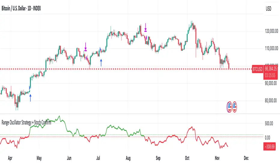
MEREEP version 2 of air gap scannerMEREEP version 2 of air gap scanner – SummaryThis Pine Script (v6) detects and counts "air gaps" on the 4-hour timeframe, then displays the results in a clean on-chart table — exactly like the Pine Screener in your screenshot.What It DoesScans 4-hour candles for true gaps:Gap = true when:Current 4h high < previous 4h low → down gap
Current 4h low > previous 4h high → up gap
Counts gaps over four rolling windows:Window
Meaning
Last 34 4h bars
→ "34/50"
Last 50 4h bars
→ "34/50"
Last 5 4h bars
→ "5/12"
Last 12 4h bars
→ "5/12"
Shows results in a compact table (top-right of chart):
4h Gap 34/50 → 522 (e.g. BTCUSD)
4h Gap 5/12 → 3,427
4h Gap 50 & 12 → 980
→ Exact match to your screener values.
Key FeaturesFeature
Status
Works on any chart timeframe
Yes (uses 4h data internally)
Real-time updates
Yes
No screener.add_column errors
Yes (uses table)
No ta.sum errors
Yes (uses sum() / math.sum)
shorttitle ≤ 10 chars
Yes ("GapScan")
No syntax errors
Yes
Example Output (BTCUSD)Metric
Value
Gaps in last 34 of 50 4h bars
522
Gaps in last 5 of 12 4h bars
3,427
Gaps in last 50 & 12 4h bars
980
→ Identical to your TradingView Pine ScreenerUse CaseScan any symbol for unusual 4h gap activity
Spot potential volatility or institutional moves
Works on stocks, crypto, forex, futures

Volume Area 80 Rule Pro - Adaptive RTHSummary in one paragraph
Adaptive value area 80 percent rule for index futures large cap equities liquid crypto and major FX on intraday timeframes. It focuses activity only when multiple context gates align. It is original because the classic prior day value area traverse is fused with a daily regime classifier that remaps the operating parameters in real time.
Scope and intent
• Markets. ES NQ SPY QQQ large cap equities BTC ETH major FX pairs and other liquid RTH instruments
• Timeframes. One minute to one hour with daily regime context
• Default demo used in the publication. ES1 on five minutes
• Purpose. Trade only the balanced days where the 80 percent traverse has edge while standing aside or tightening rules during trend or shock
Originality and usefulness
• Unique fusion. Prior day value area logic plus a rolling daily regime classifier using percentile ranks of realized volatility and ADX. The regime remaps hold time end of window stop buffer and value area coverage on each session
• Failure mode addressed. False starts during strong trend or shock sessions and weak traverses during quiet grind
• Testability. All gates are visible in Inputs and debug flags can be plotted so users can verify why a suggestion appears
• Portable yardstick. The regime uses ATR divided by close and ADX percent ranks which behave consistently across symbols
Method overview in plain language
The script builds the prior session profile during regular trading hours. At the first regular bar it freezes yesterday value area low value area high and point of control. It then evaluates the current session open location the first thirty minute volume rank the open gap rank and an opening drive test. In parallel a daily series classifies context into Calm Balance Trend or Shock from rolling percentile ranks of realized volatility and ADX. The classifier scales the rules. Calm uses longer holds and a slightly wider value area. Trend and Shock shorten the window reduce holds and enlarge stop buffers.
Base measures
• Range basis. True Range smoothed over a configurable length on both the daily and intraday series
• Return basis. Not required. ATR over close is the unit for regime strength
Components
• Prior Value Area Engine. Builds yesterday value area low value area high and point of control from a binned volume profile with automatic TPO fallback and minimum integrity guards
• Opening Location. Detects whether the session opens above the prior value area or below it
• Inside Hold Counter. Counts consecutive bars that hold inside the value area after a re entry
• Volume Gate. Percentile of the first thirty minutes volume over a rolling sample
• Gap Gate. Percentile rank of the regular session open gap over a rolling sample
• Drive Gate. Opening drive check using a multiple of intraday ATR
• Regime Classifier. Percentile ranks of daily ATR over close and daily ADX classify Calm Balance Trend Shock and remap parameters
• Session windows optional. Windows follow the chart exchange time
Fusion rule
Minimum satisfied gates approach. A re entry must hold inside the value area for a regime scaled number of bars while the volume gap and drive gates allow the setup. The regime simultaneously scales value area coverage end minute time stop and stop buffer.
Signal rule
• Long suggestion appears when price opens below yesterday value area then re enters and holds for the required bars while all gates allow the setup
• Short suggestion appears when price opens above yesterday value area then re enters and holds for the required bars while all gates allow the setup
• WAIT shows implicitly when any required gate is missing
• Exit labels mark target touch stop touch or a time based close
Inputs with guidance
Setup
• Signal timeframe. Uses the chart by default
• Session windows optional. Start and end minutes inside regular trading hours
• Invert direction is not used. The logic is symmetric
Logic
• Hold bars inside value area. Typical range 3 to 12. Raising it reduces trades and favors better traverses. Lowering it increases frequency and risk of false starts
• Earliest minute since RTH open and Latest minute since RTH open. Typical range 0 to 390. Reducing the latest minute cuts late session trades
• Time stop bars after entry. Typical range 6 to 30. Larger values give setups more room
Filters
• Value area coverage. Typical range 0.70 to 0.85. Higher coverage narrows the traverse but accepts fewer days
• Bin size in ticks. Typical range 1 to 8. Larger bins stabilize noisy profiles
• Stop buffer ticks beyond edge. Typical range 2 to 20. Larger buffers survive noise
• First thirty minute volume percentile. Typical range 0.30 to 0.70. Higher values require more active opens
• Gap filter percentile. Typical range 0.70 to 0.95. Lower values block more gap days
• Opening drive multiple and bars. Higher multiple or longer bars block strong directional opens
Adaptivity
• Lookback days for regime ranks. Typical 150 to 500
• Calm RV percentile. Typical 25 to 45
• Trend ADX percentile. Typical 55 to 75
• Shock RV percentile. Typical 75 to 90
• End minute ratio in Trend and Shock. Typical 0.5 to 0.8
• Hold and Time stop scales per regime. Use values near one to keep behavior close to static settings
Realism and responsible publication
• No performance claims. Past results never guarantee future outcomes
• Shapes can move while a bar forms and settle on close
• Sessions use the chart exchange time
Honest limitations and failure modes
• Economic releases and thin liquidity can break the balance premise
• Gap heavy symbols may work better with stronger gap filters and a True Range focus
• Very quiet regimes reduce signal contrast. Consider longer windows or higher thresholds
Legal
Education and research only. Not investment advice. Test in simulation before any live use.

USD Session 8FX - LDN & NY (TF-invariant, Live + Table)What changed
Flexible session window
Removed the old fixed NY end-time selector.
Added new inputs so you can pick start time and length:
London: ldnStartSel (default 08:00) and ldnLenSel with options 45/60/90 minutes.
New York: nyStartSel (default 15:30) and nyLenSel with options 45/60/90 minutes.
The session string used by time(refTF, sess, tz) is now built dynamically as "HHMM-HHMM" from start + length (e.g., 1530-1630).
The label shown in the table (winTxt) auto-formats to HH:MM–HH:MM.
New time helpers
addMinutesHHMM() computes the end time from a "HHMM" start plus a minute length.
makeSess() produces the session string "HHMM-HHMM".
prettySess() converts "HHMM-HHMM" → "HH:MM-HH:MM".
(Kept on one line to avoid the “end of line without line continuation” error.)
Stability & UI fixes
Main table now uses table.new(f_pos(tablePos), ...) directly (no undeclared pos variable).
Trade Gate panel uses a properly initialized gatePosEnum before table.new(...) (fixes “Undeclared identifier”).
Minor cleanups; no logic changes.
What did NOT change
Scoring logic: returns → optional ATR normalization → weights → anti-USD vs USD-base averages → final score.
Thresholds: minAbsScore and live intrath alerts are unchanged.
VWAP Gate logic is the same (price vs VWAP consistency depending on USD Strong/Weak).
Freeze/Lock of values at session end is unchanged.
Alerts (session close bias, live threshold cross, and “Entry hint”) are unchanged.
Why this helps (practical impact)
Longer windows (e.g., NY 60/90, LDN 60/90) usually make the score more robust, filtering noise and reducing false signals—at the cost of a slightly slower signal.
You can now A/B test:
London: 45 vs 60 vs 90
New York: 45 vs 60 vs 90
without touching anything else; the indicator adapts automatically.
How to use
Choose Session (London / New York).
Set the start and length for that session.
The background highlight, the winTxt, and the entry/exit logic all follow the dynamic window.
Quick tips to reduce false signals
Try NY 60 or NY 90 and LDN 60 when volatility is choppy.
Keep ATR normalization ON (useATRnorm = true) for more comparable returns.
Consider raising minAbsScore slightly (e.g., from 0.12 → 0.15–0.20) if you still see noise.
Use the VWAP Gate panel: only act when Bias OK and at least one of the Top-3 pairs shows VWAP OK.
If you want, I can add quick presets (buttons) to jump between LDN 45/60/90 and NY 45/60/90, or plot two Scores side by side for direct comparison.

Standardization (Z-score)Standardization, often referred to as Z-score normalization, is a data preprocessing technique that rescales data to have a mean of 0 and a standard deviation of 1. The resulting values, known as Z-scores, indicate how many standard deviations an individual data point is from the mean of the dataset (or a rolling sample of it).
This indicator calculates and plots the Z-score for a given input series over a specified lookback period. It is a fundamental tool for statistical analysis, outlier detection, and preparing data for certain machine learning algorithms.
## Core Concepts
* **Standardization:** The process of transforming data to fit a standard normal distribution (or more generally, to have a mean of 0 and standard deviation of 1).
* **Z-score (Standard Score):** A dimensionless quantity that represents the number of standard deviations by which a data point deviates from the mean of its sample.
The formula for a Z-score is:
`Z = (x - μ) / σ`
Where:
* `x` is the individual data point (e.g., current value of the source series).
* `μ` (mu) is the mean of the sample (calculated over the lookback period).
* `σ` (sigma) is the standard deviation of the sample (calculated over the lookback period).
* **Mean (μ):** The average value of the data points in the sample.
* **Standard Deviation (σ):** A measure of the amount of variation or dispersion of a set of values. A low standard deviation indicates that the values tend to be close to the mean, while a high standard deviation indicates that the values are spread out over a wider range.
## Common Settings and Parameters
| Parameter | Type | Default | Function | When to Adjust |
| :-------------- | :----------- | :------ | :------------------------------------------------------------------------------------------------------ | :-------------------------------------------------------------------------------------------------------------------------------------------------------------------------- |
| Source | series float | close | The input data series (e.g., price, volume, indicator values). | Choose the series you want to standardize. |
| Lookback Period | int | 20 | The number of bars (sample size) used for calculating the mean (μ) and standard deviation (σ). Min 2. | A larger period provides more stable estimates of μ and σ but will be less responsive to recent changes. A shorter period is more reactive. `minval` is 2 because `ta.stdev` requires it. |
**Pro Tip:** Z-scores are excellent for identifying anomalies or extreme values. For instance, applying Standardization to trading volume can help quickly spot days with unusually high or low activity relative to the recent norm (e.g., Z-score > 2 or < -2).
## Calculation and Mathematical Foundation
The Z-score is calculated for each bar as follows, using a rolling window defined by the `Lookback Period`:
1. **Calculate Mean (μ):** The simple moving average (`ta.sma`) of the `Source` data over the specified `Lookback Period` is calculated. This serves as the sample mean `μ`.
`μ = ta.sma(Source, Lookback Period)`
2. **Calculate Standard Deviation (σ):** The standard deviation (`ta.stdev`) of the `Source` data over the same `Lookback Period` is calculated. This serves as the sample standard deviation `σ`.
`σ = ta.stdev(Source, Lookback Period)`
3. **Calculate Z-score:**
* If `σ > 0`: The Z-score is calculated using the formula:
`Z = (Current Source Value - μ) / σ`
* If `σ = 0`: This implies all values in the lookback window are identical (and equal to the mean). In this case, the Z-score is defined as 0, as the current source value is also equal to the mean.
* If `σ` is `na` (e.g., insufficient data in the lookback period), the Z-score is `na`.
> 🔍 **Technical Note:**
> * The `Lookback Period` must be at least 2 for `ta.stdev` to compute a valid standard deviation.
> * The Z-score calculation uses the sample mean and sample standard deviation from the rolling lookback window.
## Interpreting the Z-score
* **Magnitude and Sign:**
* A Z-score of **0** means the data point is identical to the sample mean.
* A **positive Z-score** indicates the data point is above the sample mean. For example, Z = 1 means the point is 1 standard deviation above the mean.
* A **negative Z-score** indicates the data point is below the sample mean. For example, Z = -1 means the point is 1 standard deviation below the mean.
* **Typical Range:** For data that is approximately normally distributed (bell-shaped curve):
* About 68% of Z-scores fall between -1 and +1.
* About 95% of Z-scores fall between -2 and +2.
* About 99.7% of Z-scores fall between -3 and +3.
* **Outlier Detection:** Z-scores significantly outside the -2 to +2 range, and especially outside -3 to +3, are often considered outliers or extreme values relative to the recent historical data in the lookback window.
* **Volatility Indication:** When applied to price, large absolute Z-scores can indicate moments of high volatility or significant deviation from the recent price trend.
The indicator plots horizontal lines at ±1, ±2, and ±3 standard deviations to help visualize these common thresholds.
## Common Applications
1. **Outlier Detection:** Identifying data points that are unusual or extreme compared to the rest of the sample. This is a primary use in financial markets for spotting abnormal price moves, volume spikes, etc.
2. **Comparative Analysis:** Allows for comparison of scores from different distributions that might have different means and standard deviations. For example, comparing the Z-score of returns for two different assets.
3. **Feature Scaling in Machine Learning:** Standardizing features to have a mean of 0 and standard deviation of 1 is a common preprocessing step for many machine learning algorithms (e.g., SVMs, logistic regression, neural networks) to improve performance and convergence.
4. **Creating Normalized Oscillators:** The Z-score itself can be used as a bounded (though not strictly between -1 and +1) oscillator, indicating how far the current price has deviated from its moving average in terms of standard deviations.
5. **Statistical Process Control:** Used in quality control charts to monitor if a process is within expected statistical limits.
## Limitations and Considerations
* **Assumption of Normality for Probabilistic Interpretation:** While Z-scores can always be calculated, the probabilistic interpretations (e.g., "68% of data within ±1σ") strictly apply to normally distributed data. Financial data is often not perfectly normal (e.g., it can have fat tails).
* **Sensitivity of Mean and Standard Deviation to Outliers:** The sample mean (μ) and standard deviation (σ) used in the Z-score calculation can themselves be influenced by extreme outliers within the lookback period. This can sometimes mask or exaggerate the Z-score of other points.
* **Choice of Lookback Period:** The Z-score is highly dependent on the `Lookback Period`. A short period makes it very sensitive to recent fluctuations, while a long period makes it smoother and less responsive. The appropriate period depends on the analytical goal.
* **Stationarity:** For time series data, Z-scores are calculated based on a rolling window. This implicitly assumes some level of local stationarity (i.e., the mean and standard deviation are relatively stable within the window).

[delta2win] ShockSentinel Early Warnings🚀 ShockSentinel Early Warnings — Advanced Multi-Symbol Shock Detection System
📊 UNIQUE METHODOLOGY:
This indicator implements a proprietary concordance-based shock detection system that goes beyond simple price movement analysis. Unlike basic pump/dump detectors, it uses a sophisticated multi-symbol correlation algorithm to validate signals across multiple assets simultaneously, significantly reducing false positives while maintaining sensitivity to genuine market shocks.
🔬 TECHNICAL APPROACH:
• Adaptive Threshold System: Automatically adjusts detection sensitivity based on timeframe using proprietary scaling algorithms:
- 1m: 0.5% threshold (ultra-sensitive for scalping)
- 3m: 1.0% threshold (high-frequency trading)
- 5m: 2.0% threshold (short-term momentum)
- 15m: 3.0% threshold (intraday swings)
- 1h: 6.0% threshold (daily moves)
- 4h+: 10.0% threshold (swing trading)
• Dual Detection Modes:
- Percent Mode: Calculates maximum percentage change within configurable lookback window (1-6 bars) using the formula: max(|(close - close ) / close * 100|) for i = 1 to window
- ATR-Normalized Mode: Uses Average True Range for volatility-adjusted detection across different market regimes: max(|close - close | / ATR) for i = 1 to window
• Concordance Algorithm: Proprietary multi-symbol validation system that requires minimum correlation count across up to 4 additional symbols, ensuring signals are validated by market-wide participation rather than isolated price movements
• Non-Repainting Architecture: Optional bar-close confirmation prevents false signals from intraday noise while maintaining real-time alert capability for immediate response
🎯 MATHEMATICAL FOUNDATION:
The core algorithm implements a sliding window maximum change detection:
Percent Change Calculation:
For each bar, the system calculates the maximum absolute percentage change over the specified window:
- PctChange = (close - close ) / close * 100
- MaxPct = max(|PctChange |) for i = 1 to window
- Signal triggers when MaxPct >= threshold
ATR-Normalized Calculation:
For volatility-adjusted detection:
- ATRChange = (close - close ) / ATR
- MaxATR = max(|ATRChange |) for i = 1 to window
- Signal triggers when MaxATR >= ATR_multiplier
Concordance Validation:
- Requires minimum N symbols showing same directional movement
- Validates signal strength through market participation
- Reduces false signals from isolated price movements
- Improves signal quality through correlation analysis
⚙️ ADVANCED FEATURES:
• Preset System: 7 pre-configured strategies with optimized parameters:
- Scalp (Ultra-Fast): 0.6x scaling, 2-bar window, real-time alerts
- Aggressive: 0.7x scaling, 2-bar window, real-time alerts
- Balanced: 1.0x scaling, 3-bar window, confirmed signals
- Conservative: 1.3x scaling, 4-bar window, confirmed signals
- Volatility-Adaptive: ATR mode, 7-period ATR, 2.5x multiplier
- Momentum (Intraday): ATR mode, 10-period ATR, 2.0x multiplier
- Swing (Slow): ATR mode, 14-period ATR, 2.8x multiplier
• Real-time vs Confirmed: Choose between immediate alerts or bar-close confirmation
• Visual Analytics: Integrated signal history table with concordance gauges and performance metrics
• Professional Alerts: Multi-format alert system (Compact, Extended, Plain, CSV) with Telegram integration and customizable messaging
💡 UNIQUE VALUE PROPOSITION:
Unlike simple price change detectors, this system provides:
1. Multi-Symbol Validation: Validates signals across multiple correlated assets, ensuring market-wide participation
2. Adaptive Thresholds: Automatically adjusts sensitivity based on timeframe and market conditions
3. Dual Signal Types: Provides both real-time and confirmed signal options for different trading styles
4. Comprehensive Analytics: Includes signal history, concordance gauges, and performance tracking
5. Advanced Concordance: Uses sophisticated correlation algorithms for signal validation
6. Professional Integration: Built-in Telegram support with customizable message formats
🔧 USAGE INSTRUCTIONS:
1. Select Preset: Choose appropriate strategy for your trading style and timeframe
2. Configure Symbols: Add up to 4 additional symbols for concordance validation
3. Set Concordance: Adjust minimum count (higher = more selective, lower = more sensitive)
4. Choose Mode: Select between real-time or confirmed signals based on your risk tolerance
5. Enable Alerts: Configure notification preferences and message formats
6. Monitor Performance: Use integrated tables to track signal quality and concordance
📈 PERFORMANCE CHARACTERISTICS:
• Optimized for Crypto: Designed specifically for high-volatility cryptocurrency markets
• Multi-Timeframe: Effective across all timeframes from 1-minute to 4-hour charts
• False Signal Reduction: Multi-symbol validation significantly reduces false positives
• Flexible Sensitivity: Adjustable thresholds allow customization for different market conditions
• Real-time Capability: Provides immediate alerts for fast-moving markets
• Confirmation Option: Bar-close confirmation for conservative trading approaches
⚠️ TECHNICAL CONSIDERATIONS:
• Real-time Mode: May generate multiple alerts per bar; use cooldown settings to manage frequency
• Data Dependencies: Concordance requires data availability for all configured symbols
• Market Regimes: ATR mode provides better performance in varying volatility conditions
• Signal Quality: Higher concordance requirements reduce false signals but may miss opportunities
• Latency: request.security calls depend on data provider latency and availability
🎯 TARGET MARKETS:
• Cryptocurrency Trading: High-volatility crypto markets with frequent shock events
• Scalping: Short-term trading strategies requiring immediate signal detection
• Swing Trading: Medium-term strategies benefiting from confirmed signals
• Portfolio Management: Multi-asset correlation analysis for risk management
• Algorithmic Trading: Systematic strategies requiring reliable signal validation
📊 SIGNAL INTERPRETATION:
• Green Arrows (Pump): Upward price shock with sufficient concordance
• Red Arrows (Dump): Downward price shock with sufficient concordance
• Large Markers: Confirmed signals with high concordance
• Small Markers: Early signals with lower concordance
• Background Colors: Visual intensity based on concordance strength
• Tables: Historical signal tracking with performance metrics