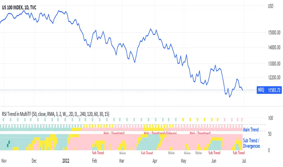
RSI Trend Heatmap in Multi TimeframesRSI Trend Heatmap in Multi Timeframes
Description
Sometimes you want to look at the RSI Trend across multiple time frames.
You have to waste time browsing through them.
So we've put together every time frame you want to see in one indicator.
We have 10 layers of RSI Trend heatmap available for you.
You can set the timeframe as you want on the Settings page.
Description of Parameter RSI Setting ** You can change it by setting.
RSI Trend Length : (Default 50)
Source : (Default close)
RSI Sideways Length : (Default 2 = RSI between 48 .. 52)
Description of Parameter RSI Timeframe ** You can change it by setting.
""=None,
"M"=1Month, "2W"=2Weeks, "W"=1Week,
"3D"=3Days, "2D"=2Days, "D"=1Day,
"720"=12Hours, "480"=4Hours, "240"=4Hours, "180"=3Hours, "120"=2Hours,
"60"=60Minutes, "30"=30Minutes, "15"=15Minutes, "5"=5Minutes, "1"=1Minute
Default Configurate of RSI Timeframe (for a time frame of 1 hour to 1 day)
"W"= Timeframe 1 month shown in line 90-100 --> Represent Long Trend of RSI
---------------------------------------
"D2"= Timeframe 2 days shown in line 70-80 --> Represent Trend of RSI
"D"= Timeframe 1 day shown in line 60-70 --> Represent Trend of RSI
---------------------------------------
"240"= Timeframe 3 hours shown in line 40-50 --> Represent Signal Up/Signal Down/Divergence of RSI
"120"= Timeframe 2 hours shown in line 30-40 --> Represent Signal Up/Signal Down/Divergence of RSI
"60"= Timeframe 1 hour shown in line 20-30 --> Represent Signal Up/Signal Down/Divergence of RSI
"30"= Timeframe 30 minutes shown in line 10-20 --> Represent Signal Up/Signal Down/Divergence of RSI
"15"= Timeframe 15 minutes shown in line 00-10 --> Represent Signal Up/Signal Down/Divergence of RSI
Description of Colors
Dark Bule = Extreme Uptrend / Overbought / Bull Market (RSI > 67)
Light Bule = Uptrend (RSI between 50-52 .. 67)
Yellow = Sideways Trend / Trend Reversal (RSI between 48 .. 52) ** You can change it by setting.
Light Red = Downtrend (RSI between 33 .. 48-50)
Dark Red = Extreme Downtrend / Oversold / Bear Market (RSI < 33)
How to use
1. You must first know what the main trend of the RSI is (look at the 60-80 line). If it is red, it is a downtrend. and if it's blue shows that it is an uptrend
2. Throughout the period of the main trend There will always be a reversal of the sub-trend. (Can see from the 0-50 line), but eventually will return to follow the main trend.
3. Unless the sub trend persists for a long time until the main trend changes.
Pesquisar nos scripts por "信达证券能涨到50元吗"
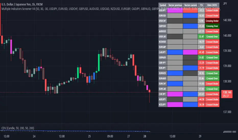
Multiple Indicator 50EMA Cross AlertsHere’s a screener including Symbol, Price, TSI, and 50 ema cross in a table output.
The 50 Exponential Moving Average is a trend indicator
You can find bullish momentum when the 50 ema crossed over or a bearish momentum when the 50 ema crossed under we are looking to take advantage by trading the reversion of these trends.
True strength index (TSI) is a trend momentum indicator
Readings are bullish when the True Strength Index shows positive values
Readings are bearish when the indicator displays negative values.
When a value is above 20, we look for selling overbought opportunity and when the value is under 20, we look for buying oversold opportunity.
You can select the pair of your choice in the settings.
Make sure to create an alert and choose any alerts then an alert will trigger when a price cross under or cross over the 50 ema for every pair separately.
This allow the user to verify if there is a trade set up or not.
Disclaimer
This post and the script don’t provide any financial advice.
ROC PercentileRate Of Change Percentile calculates the current ROC (user defined length) as a percentile rank.
We use 2 separate arrays, one for all positive ROC values and one for all negative values within a defined lookback period. Then the current ROC value is compared to those arrays to find it's percentile ranking.
For example, a ranking of 75 means the ROC is in the 75th percentile of all POSITIVE ROC values over the lookback period.
A ranking of -80 is in the 80th percentile of all NEGATIVE ROC values over the lookback period.
Most ROC scripts use raw ROC values (or smoothed or otherwise altered), or have stochastic formula applied to them, I've not seen one that displays ROC as percentile ranking of previous positive/negative values.
What is the advantage?
Raw ROC data only gives half the picture. What we want to do is compare the ROC to previous ROC values, to give a sense of scale. Raw ROC values don't give you that context and you can only compare visually, usually limited to the number of bars you can see on your screen.
Using a percentile ranking gives us the context of current Rate of Change relative to the previous Rate of Change over a large lookback period, and not just visually but mathematically.
Why not using a long stochastic ROC? The problem with stochastics in general is that an outlier data point can ruin the data for the rest of the lookback period.
For example, imagine a huge outlier 8% ROC. The 2nd largest ROC is 4% and the 3rd largest is 2%, with all other values below this.
In this example, a stochastic ROC would display the 8% outlier as 100, the 4% as 50, the 2% as 25 and all other data would be squeezed down between 0-25.
Additionally, a value of 60 may have vastly different meaning depending on whether the lookback period contains a large outlier or not.
With a percentile ranking, that 8% outlier would still have a value of 100. But the 4% and 2% would be 99 and 98 respectively (this assumes 100 data points in the series, in reality values will usually be decimals).
This effectively flattens the curve and gives a more consistent and dependable experience, allowing you to more accurately assess the relative importance of the current ROC.
The line of circles is set at the 50 and -50 values for quick comparison.
Values > 50 represent ROC greater than 50% of previous positive ROC values.
Values < -50 represent ROC greater than 50% of previous negative ROC values.

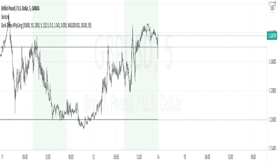
Bank Zones #PipGangHello Traders,
If you trade Forex and Indices this indicator will help you identify Buying and Selling levels that Banks are interested in. These levels are displayed on all time frames. Colors of the lines can be customized.
I also added code to show two EMA's, just uncomment the code to show them. :-)
How to use this indicator.
Show Bank Zones - this will enable/disable horizonal lines on the chart.
Price - enter bank zone price.
Increment By - plots three horizonal lines in pips above and below bank zone price.
Note: Decimal placement is KEY, this may vary by symbol.
Sample Settings:
US30USD
Price 35600.0
IncrementBy 50 (equals 50 pips)
XAUUSD
Price 1850.000
IncrementBy 5 (equals 50 pips)
GBPJPY
Price 152.500
IncrementBy .5 (equals 50 pips)
GBPUSD
Price 1.34100
IncrementBy .005 (equals 50 pips)
Forex scalper 2xEMA + SRSI + MACDThis is a forex scalping strategy designed for the most liquid pairs, like major forex pairs.
Its made of
1 EMA 50
1 EMA 100
Stochastic RSI
MACD
Rules
For long :close of the candle is above moving average 50, moving average 50> moving average 100, macd histogram is positive and cross over of stochastic rsi with the oversold level.
For short :close of the candle is below moving average 50, moving average 50 < moving average 100, macd histogram is negative and cross under of stochastic rsi with the overbought level.
Exit
For exit we have take profit and stop loss using fixed pip points.
For this example on EURUSD we use 20 pips for both tp and sl
IF you have any questions let me know !

EBB & Flow: a multi-EMA-based BB cloudIntro
This is an idea evolved out of the market maker method and EMA convergence, divergence, and mean reversion.
The market maker method informs us that the 5, 13, 50 and 200 EMAs are important to regulating price. Those EMA lengths are multiples of the 50 and 200 on lower major timeframes -- the 1 minute, 5, 15, 1H, 4H, 1D. I include the 21 because it is also a multiple and in crypto very often respected.
When market makers are testing price, they set their range and spike in the direction they test for liquidity. This can get chaotic. For instance, in a shorter time frame consolidation inside a bigger timeframe uptrend, it can be too easy to forget where you are in the many trends playing out.
When the EMAs are dragged over each other during normal price movement, you get these crisscrossing tracks of price, and the individual breaks can be hard to trace.
The range is what matters, ultimately, and the range is dynamic. In that case, the Bollinger Band is a great tool for detecting outliers in this case.
The Answer
So the answer this indicator seeks to give, is to look for outliers. This gives you a scalping strategy built on Traders Reality thinking and best put together with the PVSRA indicator, which I may include in this indicator just for the sake of concision, but they can work alongside each other or separately.
The key thing is the different EMA clouds, which are bollinger bands. Tight bands mean imminent breaks, favouring the trend. Vector candles out of a zone, pins to the low/high, etc. are all very relevant alongside this indicator.
You can also use it on its own and scalp the breaks of a cloud.
How it works
Each cloud is a standard deviation from their respective EMA, all in the same colour. The deviation multiple is 1.618 by default. Yes, fibonacci sequences are usually nonsense, but it works better with the BB than 2, 2.5 or 3.
Using just the clouds, you can see where each EMA is headed and how it behaves within the deviation of the others.
But that on its own isn't enough.
The indicator will also print snowflakes above and below the candle for notable outliers. It will be in the colour of the cloud it breaks, but only if that break is also breaking the smaller EMA clouds too.
The most snowflakes will be yellow because that's the 13 EMA. That one is dependent on nothing else and every break will print a snowflake. The 21 will be dependent on the 13. The 50 dependent on the 13 and 21 breaks. The 200 the most important.
For example, if the 200 EMA-BB or EBB is broken at the upper band, deviating by more than 162% of price over a 200 period EMA, and that break is not above the 50 EMA cloud, there will be no snowflake. However, if it exceeds the 13, 21, 50, and 200 clouds, then a purple snowflake will appear above the bar.
Any snowflake is an extreme in price. The purple is an especially good point of entry. That doesn't mean it is a perfect entry. You can build position from it, though, and be relatively certain of a price correction in the near future, because not only was this major EMA cloud violated, but all of the smaller ones too.
Reminder
You still need your PVSRA and candlesticks. This indicator on its own may have a nice hit rate for scalping and building position, as an alternative to the TDI or alongside it, but it is not enough on its own, just like the TDI.
Enjoy!

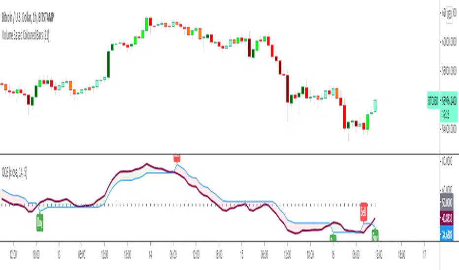
Quantitative Qualitative Estimation QQE
The QQE indicator is a momentum based indicator to determine trend and sideways.
The Qualitative Quantitative Estimation (QQE) indicator works like a smoother version of the popular Relative Strength Index (RSI) indicator. QQE expands on RSI by adding two volatility based trailing stop lines. These trailing stop lines are composed of a fast and a slow moving Average True Range (ATR). These ATR lines are smoothed making this indicator less susceptible to short term volatility.
The most common method of using QQE is to look for crosses of the fast and slow moving trailing stop lines during periods when the QQE line reflects overbought or oversold conditions
Qualitative Quantitative Estimation made up of a smoothed Relative Strength Index (RSI) indicator plus fast and slow volatility-based trailing levels.
Qualitative Quantitative Estimation can be used in two directions:
1.Determine the trend, i.e. if the line is above the 50 level, the trend is ascending, if below - descending;
2.Search for signals at the moment of crossing of the QQE FAST (maroon) and QQE SLOW (blue) lines.
The QQE itself is generally considered to indicate an up-trend ifQQE FAST is above QQE SLOW, and a down-trend if below QQE SLOW.
Often a middle-range between 40 and 60 is set and if the indicator is in that range, then the market is considered to be tracking sideways, or in no trend.
You will need to set only one parameter – “SF” "RSI SMoothing Factor", an analogue of the period in RSI.
By the way, judging from the open source information, the algorithm used the standard strength index with a period of 14 for calculations.
Various signals can be created from the indicator such as:
-Buy when QQE FAST crosses above QQE SLOW below 50 level or just buy when QQE lines crosses above 50 level.
-Sell when QQE FAST crosses below QQE SLOW above 50 level or just sell when QQE lines crosses below 50 level.
WARNING: QQE IS A RSI BASED INDICATOR SO THAT IT CAN TRIGGER FALSE SIGNALS DURING DIVERGENCES!
Kıvanç Özbilgiç
Nifty VolumeWhy this Script : Nifty 50 does not provide volume and some time it is really useful to understand the volume .
This is the pine script which calculate the nifty 50 volume .
Logic :
Take each stock contribute to nifty 50 and find it's volume .
Multiply the same with contribution percentage of the same on Nifty 50
Add up all of them and find the total volume .
There is a similar script by @daytraderph which is built for Bank Nifty (custom volume) . I took the same and built for Nfity.
Nifty has 50 stocks and you cant call security method more than 40 times from one Pine script, so this is the limitation of this script. It consider top 40 stocks and find the volume (which contribute pretty much around 95% of the volume) and convert the same to 100 %
Simple Moving Average Double HelixThis one is a mix of colour-coded moving averages and Ichimoku. It features two pairs of SMAs--default values of 9/20 and 50/200. Each SMA will be green when it rises and red when it falls. The spaces between each pair will fill with green or red depending on which line is on top. 9 over 20 or 50 over 200 makes a green cloud; if 9 or 50 falls below, the cloud will switch to green.
There's also the Ichimoku lagging span and a 35-period SMA (grey) that can be used as a trailing stop loss guideline.
Ideal long setup:
9, 20, 50, and 200 SMA are all green
both clouds are green
lagging span is above historic price action
Ideal short setup:
9, 20, 50, and 200 SMA are all red
both clouds are red
lagging span is below historic price action

RSI5_50 with DivergenceThis is variation of RSI Divergence strategy.
I have added a filter (long term RSI) to the Rules. strategy BUYs when RSI 50 period is above 50 line and there is divergence on the short term RSI
settings
=========
short term RSI period 5
long term RSI period 50
stopLoss is 8% --- if setting is enabled
BUY Rule
========
RSI 50 is above 50 line
short term RSI is showing divergence
Add to existing
==============
if already in position, BUY when shorTermRSI is crossing above 20
TakeProfit
=========
when longTermRSI reaches 60,65, 70 and 75 level , take partial profits .
(not when crossing down --- This may affect on profits , because when price goes down , it goes very fast )
Exit
=====
when longTermRSI is crossing down 30
OR stopLoss value hits
Note: When I tested this with GOOGL stock , I have got excellent results ... any experts there , please check everything is good with scripting ...
Happy Trading

PowerX Strategy Bar Coloring [OFFICIAL VERSION]This script colors the bars according to the PowerX Strategy by Markus Heitkoetter:
The PowerX Strategy uses 3 indicators:
- RSI (7)
- Stochastics (14, 3, 3)
- MACD (12, 26 , 9)
The bars are colored GREEN if...
1.) The RSI (7) is above 50 AND
2.) The Stochastic (14, 3, 3) is above 50 AND
3.) The MACD (12, 26, 9) is above its Moving Average, i.e. MACD Histogram is positive.
The bars are colored RED if...
1.) The RSI (7) is below 50 AND
2.) The Stochastic (14, 3, 3) is below 50 AND
3.) The MACD (12, 26, 9) is below its Moving Average, i.e. MACD Histogram is negative.
If only 2 of these 3 conditions are met, then the bars are black (default color)
We highly recommend plotting the indicators mentioned above on your chart, too, so that you can see when bars are getting close to being "RED" or "GREEN", e.g. RSI is getting close to the 50 line.
BO - Bar's direction Signal - BacktestingBO - Bar's direction Signal - Backtesting Options:
A. Factors Calculate probability of x bars same direction
1. Periods Counting: Data to count From day/month/year To day/month/year
2. Trading Time: only cases occurred in trading time were counted.
B. Timezone
1. Trading time depend on Time zone and specified chart.
2. Enable Highlight Trading Time to check your period time is correct
C. Date Backtesting
* Only cases occurred in Date Backtesting were reported.
D. Setup Options & Rule
1. Reversal after 2 bars same direction
* Probability of 3 bars same direction < 50
* 2 bars same direction is start of series
2. Reversal after 3 bars same direction
* Probability of 4 bars same direction < 50
* 3 bars same direction is start of series
3. Reversal after 4 bars same direction
* Probability of 4 bars same direction < 50
* 3 bars same direction is start of series
4. Reversal after 5 bars same direction
* Probability of 5 bars same direction < 50
* 4 bars same direction is start of series
5. Reversal after 6 bars same direction
* Probability of 6 bars same direction < 50
* 5 bars same direction is start of series

Technical Analysis - Panel Info//A. Oscillators & B. Moving Averages base on TradingView's Technical Analysis by ThiagoSchmitz
//C.Pivot base on Ultimate Pivot Points Alerts by elbartt
//D. Summary & Panel info by anhnguyen14
Panel Info base on these indicators:
A. Oscillators
1. Rsi (14)
2. Stochastic (14,3,3)
3. CCI (20)
4. ADX (14)
5. AO
6. Momentum (10)
7. MACD (12,26)
8. Stoch RSI (3,3,14,14)
9. %R (14)
10. Bull bear
11. UO (7,14,28)
B. Moving Averages
1. SMA & EMA: 5-10-20-30-50-100-200
2. Ichimoku Cloud - Baseline (26)
3. Hull MA (9)
C. Pivot
1. Traditional
2. Fibonacci
3. Woodie
4. Camarilla
D. Summary
Sum_red=A_red+B_red+C_red
Sum_blue=A_blue+B_blue+C_blue
sell_point=(Sum_red/32)*100
buy_point=(Sum_blue/32)*100
sell =
Sum_red>Sum_blue
and sell_point>50
Strong_sell =
A_red>A_blue
and B_red>B_blue
and C_red>C_blue
and sell_point>50
and not crossunder(sell_point,75)
buy =
Sum_red>Sum_blue
and buy_point>50
Strong_buy =
A_red50
and not crossunder(buy_point,75)
neutral = not sell and not Strong_sell and not buy and not Strong_buy

Multi SMA EMA WMA HMA BB (5x8 MAs Bollinger Bands) MAX MTF - RRBMulti SMA EMA WMA HMA 4x7 Moving Averages with Bollinger Bands MAX MTF by RagingRocketBull 2019
Version 1.0
All available MAX MTF versions are listed below (They are very similar and I don't want to publish them as separate indicators):
ver 1.0: 4x7 = 28 MTF MAs + 28 Levels + 3 BB = 59 < 64
ver 2.0: 5x6 = 30 MTF MAs + 30 Levels + 3 BB = 63 < 64
ver 3.0: 3x10 = 30 MTF MAs + 30 Levels + 3 BB = 63 < 64
ver 4.0: 5(4+1)x8 = 8 CurTF MAs + 32 MTF MAs + 20 Levels + 3 BB = 63 < 64
ver 5.0: 6(5+1)x6 = 6 CurTF MAs + 30 MTF MAs + 24 Levels + 3 BB = 63 < 64
ver 6.0: 4(3+1)x10 = 10 CurTF MAs + 30 MTF MAs + 20 Levels + 3 BB = 63 < 64
Fib numbers: 8, 13, 21, 34, 55, 89, 144, 233, 377
This indicator shows multiple MAs of any type SMA EMA WMA HMA etc with BB and MTF support, can show MAs as dynamically moving levels.
There are 4 MA groups + 1 BB group, a total of 4 TFs * 7 MAs = 28 MAs. You can assign any type/timeframe combo to a group, for example:
- EMAs 9,12,26,50,100,200,400 x H1, H4, D1, W1 (4 TFs x 7 MAs x 1 type)
- EMAs 8,13,21,30,34,50,55,89,100,144,200,233,377,400 x M15, H1 (2 TFs x 14 MAs x 1 type)
- D1 EMAs and SMAs 8,13,21,30,34,50,55,89,100,144,200,233,377,400 (1 TF x 14 MAs x 2 types)
- H1 WMAs 13,21,34,55,89,144,233; H4 HMAs 9,12,26,50,100,200,400; D1 EMAs 12,26,89,144,169,233,377; W1 SMAs 9,12,26,50,100,200,400 (4 TFs x 7 MAs x 4 types)
- +1 extra MA type/timeframe for BB
There are several versions: Simple, MTF, Pro MTF, Advanced MTF, MAX MTF and Ultimate MTF. This is the MAX MTF version. The Differences are listed below. All versions have BB
- Simple: you have 2 groups of MAs that can be assigned any type (5+5)
- MTF: +2 custom Timeframes for each group (2x5 MTF) +1 TF for BB, TF XY smoothing
- Pro MTF: 4 custom Timeframes for each group (4x3 MTF), 1 TF for BB, MA levels and show max bars back options
- Advanced MTF: +4 extra MAs/group (4x7 MTF), custom Ticker/Symbols, Timeframe <>= filter, Remove Duplicates Option
- MAX MTF: +2 subtypes/group, packed to the limit with max possible MAs/TFs: 4x7, 5x6, 3x10, 4(3+1)x10, 5(4+1)x8, 6(5+1)x6
- Ultimate MTF: +individual settings for each MA, custom Ticker/Symbols
MAX MTF version tests the limits of Pinescript trying to squeeze as many MAs/TFs as possible into a single indicator.
It's basically a maxed out Advanced version with subtypes allowing for mixed types within a group (i.e. both emas and smas in a single group/TF)
Pinescript has the following limits:
- max 40 security calls (6 calls are reserved for dupe checks and smoothing, 2 are used for BB, so only 32 calls are available)
- max 64 plot outputs (BB uses 3 outputs, so only 61 plot outputs are available)
- max 50000 (50kb) size of the compiled code
Based on those limits, you can only have the following MAs/TFs combos in a single script:
1. 4x7, 5x6, 3x10 - total number of MTF MAs must always be <= 32, and you can still have BB and Num Levels = total MAs, without any compromises
2. 5(4+1)x8, 6(5+1)x6, 4(3+1)x10 - you can use the Current Symbol/Timeframe as an extra (+1) fixed TF with the same number of MTF MAs
- you don't need to call security to display MAs on the Current Symbol/Timeframe, so the total number of MTF MAs remains the same and is still <= 32
- to fit that many MAs into the max 64 plot outputs limit you need to reduce the number of levels (not every MA Group will have corresponding levels)
Features:
- 4x7 = 28 MAs of any type
- 4x MTF groups with XY step line smoothing
- +1 extra TF/type for BB MAs
- 2 MA subtypes within each group/TF
- 4x7 = 28 MA levels with adjustable group offsets, indents and shift
- supports any existing type of MA: SMA, EMA, WMA, Hull Moving Average (HMA)
- custom tickers/symbols for each group
- show max bars back option
- show/hide both groups of MAs/levels/BB and individual MAs
- timeframe filter: show only MAs/Levels with TFs <>= Current TF
- hide MAs/Levels with duplicate TFs
- support for custom TFs that are not available in free accounts: 2D, 3D etc
- support for timeframes in H: H, 2H, 4H etc
Notes:
- Uses timeframe textbox instead of input resolution dropdown to allow for 240 120 and other custom TFs
- Uses symbol textbox instead of input symbol to avoid establishing multiple dummy security connections to the current ticker - otherwise empty symbols will prevent script from running
- Possible reasons for missing MAs on a chart:
- there may not be enough bars in history to start plotting it. For example, W1 EMA200 needs at least 200 bars on a weekly chart.
- for charts with low/fractional prices i.e. 0.00002 << 0.001 (default Y smoothing step) decrease Y smoothing as needed (set Y = 0.0000001) or disable it completely (set X,Y to 0,0)
- for charts with high price values i.e. 20000 >> 0.001 increase Y smoothing as needed (set Y = 10-20). Higher values exceeding MAs point density will cause it to disappear as there will be no points to plot. Different TFs may require diff adjustments
- TradingView Replay Mode UI and Pinescript security calls are limited to TFs >= D (D,2D,W,MN...) for free accounts
- attempting to plot any TF < D1 in Replay Mode will only result in straight lines, but all TFs will work properly in history and real-time modes. This is not a bug.
- Max Bars Back (num_bars) is limited to 5000 for free accounts (10000 for paid), will show error when exceeded. To plot on all available history set to 0 (default)
- Slow load/redraw times. This indicator becomes slower, its UI less responsive when:
- Pinescript Node.js graphics library is too slow and inefficient at plotting bars/objects in a browser window. Code optimization doesn't help much - the graphics engine is the main reason for general slowness.
- the chart has a long history (10000+ bars) in a browser's cache (you have scrolled back a couple of screens in a max zoom mode).
- Reload the page/Load a fresh chart and then apply the indicator or
- Switch to another Timeframe (old TF history will still remain in cache and that TF will be slow)
- in max possible zoom mode around 4500 bars can fit on 1 screen - this also slows down responsiveness. Reset Zoom level
- initial load and redraw times after a param change in UI also depend on TF. For example: D1/W1 - 2 sec, H1/H4 - 5-6 sec, M30 - 10 sec, M15/M5 - 4 sec, M1 - 5 sec. M30 usually has the longest history (up to 16000 bars) and W1 - the shortest (1000 bars).
- when indicator uses more MAs (plots) and timeframes it will redraw slower. Seems that up to 5 Timeframes is acceptable, but 6+ Timeframes can become very slow.
- show_last=last_bars plot limit doesn't affect load/redraw times, so it was removed from MA plot
- Max Bars Back (num_bars) default/custom set UI value doesn't seem to affect load/redraw times
- In max zoom mode all dynamic levels disappear (they behave like text)
- Dupe check includes symbol: symbol, tf, both subtypes - all must match for a duplicate group
- For the dupe check to work correctly a custom symbol must always include an exchange prefix. BB is not checked for dupes
Good Luck! Feel free to learn from/reuse the code to build your own indicators.

Multi SMA EMA WMA HMA BB (4x5 MAs Bollinger Bands) Adv MTF - RRBMulti SMA EMA WMA HMA 4x5 Moving Averages with Bollinger Bands Advanced MTF by RagingRocketBull 2019
Version 1.0
This indicator shows multiple MAs of any type SMA EMA WMA HMA etc with BB and MTF support, can show MAs as dynamically moving levels.
There are 4 MA groups + 1 BB group, a total of 4 TFs * 5 MAs = 20 MAs. You can assign any type/timeframe combo to a group, for example:
- EMAs 12,26,50,100,200 x H1, H4, D1, W1 (4 TFs x 5 MAs x 1 type)
- EMAs 8,10,13,21,30,50,55,100,200,400 x M15, H1 (2 TFs x 10 MAs x 1 type)
- D1 EMAs and SMAs 8,10,12,26,30,50,55,100,200,400 (1 TF x 10 MAs x 2 types)
- H1 WMAs 7,77,89,167,231; H4 HMAs 12,26,50,100,200; D1 EMAs 89,144,169,233,377; W1 SMAs 12,26,50,100,200 (4 TFs x 5 MAs x 4 types)
- +1 extra MA type/timeframe for BB
There are several versions: Simple, MTF, Pro MTF, Advanced MTF and Ultimate MTF. This is the Advanced MTF version. The Differences are listed below. All versions have BB
- Simple: you have 2 groups of MAs that can be assigned any type (5+5)
- MTF: +2 custom Timeframes for each group (2x5 MTF) +1 TF for BB, TF XY smoothing
- Pro MTF: 4 custom Timeframes for each group (4x3 MTF), 1 TF for BB, MA levels and show max bars back options
- Advanced MTF: +2 extra MAs/group (4x5 MTF), custom Ticker/Symbols, Timeframe <>= filter, Remove Duplicates Option
- Ultimate MTF: +individual settings for each MA, custom Ticker/Symbols
Features:
- 4x5 = 20 MAs of any type
- 4x MTF groups with XY step line smoothing
- +1 extra TF/type for BB MAs
- 4x5 = 20 MA levels with adjustable group offsets, indents and shift
- supports any existing type of MA: SMA, EMA, WMA, Hull Moving Average (HMA)
- custom tickers/symbols for each group - you can compare MAs of the same symbol across exchanges
- show max bars back option
- show/hide both groups of MAs/levels/BB and individual MAs
- timeframe filter: show only MAs/Levels with TFs <>= Current TF
- hide MAs/Levels with duplicate TFs
- support for custom TFs that are not available in free accounts: 2D, 3D etc
- support for timeframes in H: H, 2H, 4H etc
Notes:
- Uses timeframe textbox instead of input resolution dropdown to allow for 240 120 and other custom TFs
- Uses symbol textbox instead of input symbol to avoid establishing multiple dummy security connections to the current ticker - otherwise empty symbols will prevent script from running
- Possible reasons for missing MAs on a chart:
- there may not be enough bars in history to start plotting it. For example, W1 EMA200 needs at least 200 bars on a weekly chart.
- price << default Y smoothing step 5. For charts with low/fractional prices (i.e. 0.00002 << 5) adjust X Y smoothing as needed (set Y = 0.0000001) or disable it completely (set X,Y to 0,0)
- TradingView Replay Mode UI and Pinescript security calls are limited to TFs >= D (D,2D,W,MN...) for free accounts
- attempting to plot any TF < D1 in Replay Mode will only result in straight lines, but all TFs will work properly in history and real-time modes. This is not a bug.
- Max Bars Back (num_bars) is limited to 5000 for free accounts (10000 for paid), will show error when exceeded. To plot on all available history set to 0 (default)
- Slow load/redraw times. This indicator becomes slower, its UI less responsive when:
- Pinescript Node.js graphics library is too slow and inefficient at plotting bars/objects in a browser window. Code optimization doesn't help much - the graphics engine is the main reason for general slowness.
- the chart has a long history (10000+ bars) in a browser's cache (you have scrolled back a couple of screens in a max zoom mode).
- Reload the page/Load a fresh chart and then apply the indicator or
- Switch to another Timeframe (old TF history will still remain in cache and that TF will be slow)
- in max possible zoom mode around 4500 bars can fit on 1 screen - this also slows down responsiveness. Reset Zoom level
- initial load and redraw times after a param change in UI also depend on TF. For example:
D1/W1 - 2 sec, H1/H4 - 5-6 sec, M30 - 10 sec, M15/M5 - 4 sec, M1 - 5 sec.
M30 usually has the longest history (up to 16000 bars) and W1 - the shortest (1000 bars).
- when indicator uses more MAs (plots) and timeframes it will redraw slower. Seems that up to 5 Timeframes is acceptable, but 6+ Timeframes can become very slow.
- show_last=last_bars plot limit doesn't affect load/redraw times, so it was removed from MA plot
- Max Bars Back (num_bars) default/custom set UI value doesn't seem to affect load/redraw times
- In max zoom mode all dynamic levels disappear (they behave like text)
1. based on 3EmaBB, uses plot*, barssince and security functions
2. you can't set certain constants from input due to Pinescript limitations - change the code as needed, recompile and use as a private version
3. Levels = trackprice implementation
4. Show Max Bars Back = show_last implementation
5. swma has a fixed length = 4, alma and linreg have additional offset and smoothing params
6. Smoothing is applied by default for visual aesthetics on MTF. To use exact ma mtf values (lines with stair stepping) - disable it
Good Luck! You can explore, modify/reuse the code to build your own indicators.
BB Quick Fire5 Bollinger Bands in levels 50,2.0 | 50,2.5 |50,3.0 |50,3.5 |50,4.0
This is used to identify pullbakcs and future pitchfork's.

CM Stochastic POP Method 2-Jake Bernstein_V1Yesterday Jake Bernstein authorized me to post his updated results with the Stochastic Pop Trading System he developed many years ago.
You can take a look at the Original System with Updated Settings at
This indicator is a different set of rules Jake mentioned in the PDF he allowed me to post.
To view the PDF use this link:
dl.dropboxusercontent.com
Today we’re releasing the version described in the PDF that uses the StochK values of 55, 50, and 45. The rules are discussed in the PDF but here is a simple breakdown:
Enter Long when StochK is below 50 and Crosses Above 55
Exit Long on Cross Below 55
Enter Short when StochK is Above 50 and crosses Below 45
Exit Short on Cross Above 45
Two Important Items to understand about this method:
To code the rules Precisely we need a function that will be available when Strategy Capabilities are released on TradingView.
There is one of Jakes Profit Maximizing Strategies that needs to be integrated with this code…which again we need the Strategy based Function that will be coming soon.
To Compare this system to the Stochastic Pop Method 1 System shown yesterday at I used the same Symbol and dates for you to compare…but remember to give this Method 2 System a Fair Look/Evaluation…we need the Soon To Be Released…TradingView Strategy Capabilities.
BackTesting Results Example: EUR-USD Daily Chart Since 01/01/2005
Strategy 1 – Stochastic Pop Method 2 System:
Go Long When Stochasticis below 50 and Crosses Above 55. Go Short When Stochastic is above 50 and Crosses Below 45. Exit Long/Short When Stochastic has a Reverse Cross of Entry Value.
Results:
Total Trades = 151
Profit = 40,758 Pips
Win% = 37.1%
Profit Factor = 1.26
Avg Trade = 270 Pips Profit
***Most Consecutive Wins = 4 ... Most Consecutive Losses = 7
Strategy 2:
Rules - Proprietary Optimization Jake Will Teach. Only Added 1 Additional Exit Rule.
Results:
Total Trades = 151
Profit = 60.305 Pips
Win% = 37.1%
Profit Factor = 1.38
Avg Trade = 399 Pips Profit
***Most Consecutive Wins = 4 ... Most Consecutive Losses = 7
Indicator Includes:
-Ability to Color Candles (CheckBox In Inputs Tab)
Green = Long Trade
Blue = No Trade
Red = Short Trade
Jake Bernstein will be a contributor on TradingView when Backtesting/Strategies are released. Jake is one of the Top Trading System Developers in the world with 45+ years experience and he is going to teach TradingView.com’s community how to create Trading Systems and how to Optimize the correct way.
Link To PDF:
dl.dropboxusercontent.com
Link to Original Version of Indicator with Updated Settings.

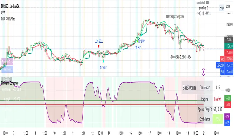
BioSwarm Imprinter™BioSwarm Imprinter™ — Agent-Based Consensus for Traders
What it is
BioSwarm Imprinter™ is a non-repainting, agent-based sentiment oscillator. It fuses many short-to-medium lookback “opinions” into one 0–100 consensus line that is easy to read at a glance (50 = neutral, >55 bullish bias, <45 bearish bias). The engine borrows from swarm intelligence: many simple voters (agents) adapt their influence over time based on how well they’ve been predicting price, so the crowd gets smarter as conditions change.
Use it to:
• Detect emerging trends sooner without overreacting to noise.
• Filter mean-reversion vs continuation opportunities.
• Gate entries with a confidence score that reflects both strength and persistence of the move.
• Combine with your execution tools (VWAP/ORB/levels) as a state filter rather than a trade signal by itself.
⸻
Why it’s different
• Swarm learning: Each agent improves or decays its “fitness” depending on whether its vote matched the next bar’s direction. High-fitness agents matter more; weak agents fade.
• Multi-horizon by design: The crowd is composed of fixed, simple lookbacks spread from lenMin to lenMax. You get a blended, robust view instead of a single fragile parameter.
• Two complementary lenses: Each agent evaluates RSI-style balance (via Wilder’s RMA) and momentum (EMA deviation). You decide the weight of each.
• No repaint, no MTF pitfalls: Everything runs on the chart’s timeframe with bar-close confirmation; no request.security() or forward references.
• Actionable UI: A clean consensus line, optional regime background, confidence heat, and triangle markers when thresholds are crossed.
⸻
What you see on the chart
• Consensus line (0–100): Smoothed to your preference; color/area makes bull/bear zones obvious.
• Regime coloring (optional): Light green in bull zone, light red in bear zone; neutral otherwise.
• Confidence heat: A small gauge/number (0–100) that combines distance from neutral and recent persistence.
• Markers (optional): Triangles when consensus crosses up through your bull threshold (e.g., 55) or down through your bear threshold (e.g., 45).
• Info panel (optional): Consensus value, regime, confidence, number of agents, and basic diagnostics.
⸻
How it works (under the hood)
1. Horizon bins: The range is divided into numBins. Each bin has a fixed, simple integer length (crucial for Pine’s safety rules).
2. Per-bin features (computed every bar):
• RSI-style balance using Wilder’s RMA (not ta.rsi()), then mapped to −1…+1.
• Momentum as (close − EMA(L)) / EMA(L) (dimensionless drift).
3. Agent vote: For its assigned bin, an agent forms a weighted score: score = wRSI*RSI_like + wMOM*Momentum. A small dead-band near zero suppresses chop; votes are +1/−1/0.
4. Fitness update (bar close): If the agent’s previous vote agreed with the next bar’s direction, multiply its fitness by learnGain; otherwise by learnPain. Fitness is clamped so it never explodes or dies.
5. Consensus: Weighted average of all votes using fitness as weights → map to 0–100 and smooth with EMA.
Why it doesn’t repaint:
• No future references, no MTF resampling, fitness updates only on confirmed bars.
• All TA primitives (RMA/EMA/deltas) are computed every bar unconditionally.
⸻
Signals & confidence
• Bullish bias: consensus ≥ bullThr (e.g., 55).
• Bearish bias: consensus ≤ bearThr (e.g., 45).
• Confidence (0–100):
• Distance score: how far consensus is from 50.
• Momentum score: how strong the recent change is versus its recent average.
• Combined into a single gate; start filtering entries at ≥60 for higher quality.
Tip: For range sessions, raise thresholds (60/40) and increase smoothing; for momentum sessions, lower smoothing and keep thresholds at 55/45.
⸻
Inputs you’ll actually tune
• Agents & horizons:
• N_agents (e.g., 64–128)
• lenMin / lenMax (e.g., 6–30 intraday, 10–60 swing)
• numBins (e.g., 12–24)
• Weights & smoothing:
• wRSI vs wMOM (e.g., 0.7/0.3 for FX & indices; 0.6/0.4 for crypto)
• deadBand (0.03–0.08)
• consSmooth (3–8)
• Thresholds & hygiene:
• bullThr/bearThr (55/45 default)
• cooldownBars to avoid signal spam
⸻
Playbooks (ready-to-use)
1) Breakout / Trend continuation
• Timeframe: 15m–1h for day/swing.
• Filter: Take longs only when consensus > 55 and confidence ≥ 60.
• Execution: Use your ORB/VWAP/pullback trigger for entry. Trail with swing lows or 1.5×ATR. Exit on a close back under 50 or when a bearish signal prints.
2) Mean reversion (fade)
• When: Sideways days or low-volatility clusters.
• Setup: Increase deadBand and consSmooth.
• Signal: Bearish fades when consensus rolls over below ≈55 but stays above 50; bullish fades when it rolls up above ≈45 but stays below 50.
• Targets: The neutral zone (~50) as the first take-profit.
3) Multi-TF alignment
• Keep BioSwarm on 1H for bias, execute on 5–15m:
• Only take entries in the direction of the 1H consensus.
• Skip counter-bias scalps unless confidence is very low (explicit mean-reversion plan).
⸻
Integrations that work
• DynamoSent Pro+ (macro bias): Only act when macro bias and swarm consensus agree.
• ORB + Session VWAP Pro: Trade London/NY ORB breakouts that retest while consensus >55 (long) or <45 (short).
• Levels/Orderflow: BioSwarm is your “go / no-go”; execution stays with your usual triggers.
⸻
Quick start
1. Drop the indicator on a 1H chart.
2. Start with: N_agents=64, lenMin=6, lenMax=30, numBins=16, deadBand=0.06, consSmooth=5, thresholds 55/45.
3. Trade only when confidence ≥ 60.
4. Add your favorite execution tool (VWAP/levels/OR) for entries & exits.
⸻
Non-repainting & safety notes
• No request.security(); no hidden lookahead.
• Bar-close confirmation for fitness and signals.
• All TA calls are unconditional (no “sometimes called” warnings).
• No series-length inputs to RSI/EMA — we use RMA/EMA formulas that accept fixed simple ints per bin.
⸻
Known limits & tips
• Too many signals? Raise deadBand, increase consSmooth, widen thresholds to 60/40.
• Too few signals? Lower deadBand, reduce consSmooth, narrow thresholds to 53/47.
• Over-fitting risk: Keep learnGain/learnPain modest (e.g., ×1.04 / ×0.96).
• Compute load: Large N_agents × numBins is heavier; scale to your device.
⸻
Example recipes
EURUSD 1H (swing):
lenMin=8, lenMax=34, numBins=16, wRSI=0.7, wMOM=0.3, deadBand=0.06, consSmooth=6, thr=55/45
Buy breakouts when consensus >55 and confidence ≥60; confirm with 5–15m pullback to VWAP or level.
SPY 15m (US session):
lenMin=6, lenMax=24, numBins=12, consSmooth=4, deadBand=0.05
On trend days, stay with longs as long as consensus >55; add on shallow pullbacks.
BTC 1H (24/7):
Increase momentum weight: wRSI=0.6, wMOM=0.4, extend lenMax to ~50. Use dynamic stops (ATR) and partials on strong verticals.
⸻
Final word
BioSwarm is a state engine: it tells you when the market is primed to continue or mean-revert. Pair it with your entries and risk framework to turn that state into trades. If you’d like, I can supply a companion strategy template that consumes the consensus and back-tests the three playbooks (Breakout/Fade/Flip) with standard risk management.
Small Business Economic Conditions - Statistical Analysis ModelThe Small Business Economic Conditions Statistical Analysis Model (SBO-SAM) represents an econometric approach to measuring and analyzing the economic health of small business enterprises through multi-dimensional factor analysis and statistical methodologies. This indicator synthesizes eight fundamental economic components into a composite index that provides real-time assessment of small business operating conditions with statistical rigor. The model employs Z-score standardization, variance-weighted aggregation, higher-order moment analysis, and regime-switching detection to deliver comprehensive insights into small business economic conditions with statistical confidence intervals and multi-language accessibility.
1. Introduction and Theoretical Foundation
The development of quantitative models for assessing small business economic conditions has gained significant importance in contemporary financial analysis, particularly given the critical role small enterprises play in economic development and employment generation. Small businesses, typically defined as enterprises with fewer than 500 employees according to the U.S. Small Business Administration, constitute approximately 99.9% of all businesses in the United States and employ nearly half of the private workforce (U.S. Small Business Administration, 2024).
The theoretical framework underlying the SBO-SAM model draws extensively from established academic research in small business economics and quantitative finance. The foundational understanding of key drivers affecting small business performance builds upon the seminal work of Dunkelberg and Wade (2023) in their analysis of small business economic trends through the National Federation of Independent Business (NFIB) Small Business Economic Trends survey. Their research established the critical importance of optimism, hiring plans, capital expenditure intentions, and credit availability as primary determinants of small business performance.
The model incorporates insights from Federal Reserve Board research, particularly the Senior Loan Officer Opinion Survey (Federal Reserve Board, 2024), which demonstrates the critical importance of credit market conditions in small business operations. This research consistently shows that small businesses face disproportionate challenges during periods of credit tightening, as they typically lack access to capital markets and rely heavily on bank financing.
The statistical methodology employed in this model follows the econometric principles established by Hamilton (1989) in his work on regime-switching models and time series analysis. Hamilton's framework provides the theoretical foundation for identifying different economic regimes and understanding how economic relationships may vary across different market conditions. The variance-weighted aggregation technique draws from modern portfolio theory as developed by Markowitz (1952) and later refined by Sharpe (1964), applying these concepts to economic indicator construction rather than traditional asset allocation.
Additional theoretical support comes from the work of Engle and Granger (1987) on cointegration analysis, which provides the statistical framework for combining multiple time series while maintaining long-term equilibrium relationships. The model also incorporates insights from behavioral economics research by Kahneman and Tversky (1979) on prospect theory, recognizing that small business decision-making may exhibit systematic biases that affect economic outcomes.
2. Model Architecture and Component Structure
The SBO-SAM model employs eight orthogonalized economic factors that collectively capture the multifaceted nature of small business operating conditions. Each component is normalized using Z-score standardization with a rolling 252-day window, representing approximately one business year of trading data. This approach ensures statistical consistency across different market regimes and economic cycles, following the methodology established by Tsay (2010) in his treatment of financial time series analysis.
2.1 Small Cap Relative Performance Component
The first component measures the performance of the Russell 2000 index relative to the S&P 500, capturing the market-based assessment of small business equity valuations. This component reflects investor sentiment toward smaller enterprises and provides a forward-looking perspective on small business prospects. The theoretical justification for this component stems from the efficient market hypothesis as formulated by Fama (1970), which suggests that stock prices incorporate all available information about future prospects.
The calculation employs a 20-day rate of change with exponential smoothing to reduce noise while preserving signal integrity. The mathematical formulation is:
Small_Cap_Performance = (Russell_2000_t / S&P_500_t) / (Russell_2000_{t-20} / S&P_500_{t-20}) - 1
This relative performance measure eliminates market-wide effects and isolates the specific performance differential between small and large capitalization stocks, providing a pure measure of small business market sentiment.
2.2 Credit Market Conditions Component
Credit Market Conditions constitute the second component, incorporating commercial lending volumes and credit spread dynamics. This factor recognizes that small businesses are particularly sensitive to credit availability and borrowing costs, as established in numerous Federal Reserve studies (Bernanke and Gertler, 1995). Small businesses typically face higher borrowing costs and more stringent lending standards compared to larger enterprises, making credit conditions a critical determinant of their operating environment.
The model calculates credit spreads using high-yield bond ETFs relative to Treasury securities, providing a market-based measure of credit risk premiums that directly affect small business borrowing costs. The component also incorporates commercial and industrial loan growth data from the Federal Reserve's H.8 statistical release, which provides direct evidence of lending activity to businesses.
The mathematical specification combines these elements as:
Credit_Conditions = α₁ × (HYG_t / TLT_t) + α₂ × C&I_Loan_Growth_t
where HYG represents high-yield corporate bond ETF prices, TLT represents long-term Treasury ETF prices, and C&I_Loan_Growth represents the rate of change in commercial and industrial loans outstanding.
2.3 Labor Market Dynamics Component
The Labor Market Dynamics component captures employment cost pressures and labor availability metrics through the relationship between job openings and unemployment claims. This factor acknowledges that labor market tightness significantly impacts small business operations, as these enterprises typically have less flexibility in wage negotiations and face greater challenges in attracting and retaining talent during periods of low unemployment.
The theoretical foundation for this component draws from search and matching theory as developed by Mortensen and Pissarides (1994), which explains how labor market frictions affect employment dynamics. Small businesses often face higher search costs and longer hiring processes, making them particularly sensitive to labor market conditions.
The component is calculated as:
Labor_Tightness = Job_Openings_t / (Unemployment_Claims_t × 52)
This ratio provides a measure of labor market tightness, with higher values indicating greater difficulty in finding workers and potential wage pressures.
2.4 Consumer Demand Strength Component
Consumer Demand Strength represents the fourth component, combining consumer sentiment data with retail sales growth rates. Small businesses are disproportionately affected by consumer spending patterns, making this component crucial for assessing their operating environment. The theoretical justification comes from the permanent income hypothesis developed by Friedman (1957), which explains how consumer spending responds to both current conditions and future expectations.
The model weights consumer confidence and actual spending data to provide both forward-looking sentiment and contemporaneous demand indicators. The specification is:
Demand_Strength = β₁ × Consumer_Sentiment_t + β₂ × Retail_Sales_Growth_t
where β₁ and β₂ are determined through principal component analysis to maximize the explanatory power of the combined measure.
2.5 Input Cost Pressures Component
Input Cost Pressures form the fifth component, utilizing producer price index data to capture inflationary pressures on small business operations. This component is inversely weighted, recognizing that rising input costs negatively impact small business profitability and operating conditions. Small businesses typically have limited pricing power and face challenges in passing through cost increases to customers, making them particularly vulnerable to input cost inflation.
The theoretical foundation draws from cost-push inflation theory as described by Gordon (1988), which explains how supply-side price pressures affect business operations. The model employs a 90-day rate of change to capture medium-term cost trends while filtering out short-term volatility:
Cost_Pressure = -1 × (PPI_t / PPI_{t-90} - 1)
The negative weighting reflects the inverse relationship between input costs and business conditions.
2.6 Monetary Policy Impact Component
Monetary Policy Impact represents the sixth component, incorporating federal funds rates and yield curve dynamics. Small businesses are particularly sensitive to interest rate changes due to their higher reliance on variable-rate financing and limited access to capital markets. The theoretical foundation comes from monetary transmission mechanism theory as developed by Bernanke and Blinder (1992), which explains how monetary policy affects different segments of the economy.
The model calculates the absolute deviation of federal funds rates from a neutral 2% level, recognizing that both extremely low and high rates can create operational challenges for small enterprises. The yield curve component captures the shape of the term structure, which affects both borrowing costs and economic expectations:
Monetary_Impact = γ₁ × |Fed_Funds_Rate_t - 2.0| + γ₂ × (10Y_Yield_t - 2Y_Yield_t)
2.7 Currency Valuation Effects Component
Currency Valuation Effects constitute the seventh component, measuring the impact of US Dollar strength on small business competitiveness. A stronger dollar can benefit businesses with significant import components while disadvantaging exporters. The model employs Dollar Index volatility as a proxy for currency-related uncertainty that affects small business planning and operations.
The theoretical foundation draws from international trade theory and the work of Krugman (1987) on exchange rate effects on different business segments. Small businesses often lack hedging capabilities, making them more vulnerable to currency fluctuations:
Currency_Impact = -1 × DXY_Volatility_t
2.8 Regional Banking Health Component
The eighth and final component, Regional Banking Health, assesses the relative performance of regional banks compared to large financial institutions. Regional banks traditionally serve as primary lenders to small businesses, making their health a critical factor in small business credit availability and overall operating conditions.
This component draws from the literature on relationship banking as developed by Boot (2000), which demonstrates the importance of bank-borrower relationships, particularly for small enterprises. The calculation compares regional bank performance to large financial institutions:
Banking_Health = (Regional_Banks_Index_t / Large_Banks_Index_t) - 1
3. Statistical Methodology and Advanced Analytics
The model employs statistical techniques to ensure robustness and reliability. Z-score normalization is applied to each component using rolling 252-day windows, providing standardized measures that remain consistent across different time periods and market conditions. This approach follows the methodology established by Engle and Granger (1987) in their cointegration analysis framework.
3.1 Variance-Weighted Aggregation
The composite index calculation utilizes variance-weighted aggregation, where component weights are determined by the inverse of their historical variance. This approach, derived from modern portfolio theory, ensures that more stable components receive higher weights while reducing the impact of highly volatile factors. The mathematical formulation follows the principle that optimal weights are inversely proportional to variance, maximizing the signal-to-noise ratio of the composite indicator.
The weight for component i is calculated as:
w_i = (1/σᵢ²) / Σⱼ(1/σⱼ²)
where σᵢ² represents the variance of component i over the lookback period.
3.2 Higher-Order Moment Analysis
Higher-order moment analysis extends beyond traditional mean and variance calculations to include skewness and kurtosis measurements. Skewness provides insight into the asymmetry of the sentiment distribution, while kurtosis measures the tail behavior and potential for extreme events. These metrics offer valuable information about the underlying distribution characteristics and potential regime changes.
Skewness is calculated as:
Skewness = E / σ³
Kurtosis is calculated as:
Kurtosis = E / σ⁴ - 3
where μ represents the mean and σ represents the standard deviation of the distribution.
3.3 Regime-Switching Detection
The model incorporates regime-switching detection capabilities based on the Hamilton (1989) framework. This allows for identification of different economic regimes characterized by distinct statistical properties. The regime classification employs percentile-based thresholds:
- Regime 3 (Very High): Percentile rank > 80
- Regime 2 (High): Percentile rank 60-80
- Regime 1 (Moderate High): Percentile rank 50-60
- Regime 0 (Neutral): Percentile rank 40-50
- Regime -1 (Moderate Low): Percentile rank 30-40
- Regime -2 (Low): Percentile rank 20-30
- Regime -3 (Very Low): Percentile rank < 20
3.4 Information Theory Applications
The model incorporates information theory concepts, specifically Shannon entropy measurement, to assess the information content of the sentiment distribution. Shannon entropy, as developed by Shannon (1948), provides a measure of the uncertainty or information content in a probability distribution:
H(X) = -Σᵢ p(xᵢ) log₂ p(xᵢ)
Higher entropy values indicate greater unpredictability and information content in the sentiment series.
3.5 Long-Term Memory Analysis
The Hurst exponent calculation provides insight into the long-term memory characteristics of the sentiment series. Originally developed by Hurst (1951) for analyzing Nile River flow patterns, this measure has found extensive application in financial time series analysis. The Hurst exponent H is calculated using the rescaled range statistic:
H = log(R/S) / log(T)
where R/S represents the rescaled range and T represents the time period. Values of H > 0.5 indicate long-term positive autocorrelation (persistence), while H < 0.5 indicates mean-reverting behavior.
3.6 Structural Break Detection
The model employs Chow test approximation for structural break detection, based on the methodology developed by Chow (1960). This technique identifies potential structural changes in the underlying relationships by comparing the stability of regression parameters across different time periods:
Chow_Statistic = (RSS_restricted - RSS_unrestricted) / RSS_unrestricted × (n-2k)/k
where RSS represents residual sum of squares, n represents sample size, and k represents the number of parameters.
4. Implementation Parameters and Configuration
4.1 Language Selection Parameters
The model provides comprehensive multi-language support across five languages: English, German (Deutsch), Spanish (Español), French (Français), and Japanese (日本語). This feature enhances accessibility for international users and ensures cultural appropriateness in terminology usage. The language selection affects all internal displays, statistical classifications, and alert messages while maintaining consistency in underlying calculations.
4.2 Model Configuration Parameters
Calculation Method: Users can select from four aggregation methodologies:
- Equal-Weighted: All components receive identical weights
- Variance-Weighted: Components weighted inversely to their historical variance
- Principal Component: Weights determined through principal component analysis
- Dynamic: Adaptive weighting based on recent performance
Sector Specification: The model allows for sector-specific calibration:
- General: Broad-based small business assessment
- Retail: Emphasis on consumer demand and seasonal factors
- Manufacturing: Enhanced weighting of input costs and currency effects
- Services: Focus on labor market dynamics and consumer demand
- Construction: Emphasis on credit conditions and monetary policy
Lookback Period: Statistical analysis window ranging from 126 to 504 trading days, with 252 days (one business year) as the optimal default based on academic research.
Smoothing Period: Exponential moving average period from 1 to 21 days, with 5 days providing optimal noise reduction while preserving signal integrity.
4.3 Statistical Threshold Parameters
Upper Statistical Boundary: Configurable threshold between 60-80 (default 70) representing the upper significance level for regime classification.
Lower Statistical Boundary: Configurable threshold between 20-40 (default 30) representing the lower significance level for regime classification.
Statistical Significance Level (α): Alpha level for statistical tests, configurable between 0.01-0.10 with 0.05 as the standard academic default.
4.4 Display and Visualization Parameters
Color Theme Selection: Eight professional color schemes optimized for different user preferences and accessibility requirements:
- Gold: Traditional financial industry colors
- EdgeTools: Professional blue-gray scheme
- Behavioral: Psychology-based color mapping
- Quant: Value-based quantitative color scheme
- Ocean: Blue-green maritime theme
- Fire: Warm red-orange theme
- Matrix: Green-black technology theme
- Arctic: Cool blue-white theme
Dark Mode Optimization: Automatic color adjustment for dark chart backgrounds, ensuring optimal readability across different viewing conditions.
Line Width Configuration: Main index line thickness adjustable from 1-5 pixels for optimal visibility.
Background Intensity: Transparency control for statistical regime backgrounds, adjustable from 90-99% for subtle visual enhancement without distraction.
4.5 Alert System Configuration
Alert Frequency Options: Three frequency settings to match different trading styles:
- Once Per Bar: Single alert per bar formation
- Once Per Bar Close: Alert only on confirmed bar close
- All: Continuous alerts for real-time monitoring
Statistical Extreme Alerts: Notifications when the index reaches 99% confidence levels (Z-score > 2.576 or < -2.576).
Regime Transition Alerts: Notifications when statistical boundaries are crossed, indicating potential regime changes.
5. Practical Application and Interpretation Guidelines
5.1 Index Interpretation Framework
The SBO-SAM index operates on a 0-100 scale with statistical normalization ensuring consistent interpretation across different time periods and market conditions. Values above 70 indicate statistically elevated small business conditions, suggesting favorable operating environment with potential for expansion and growth. Values below 30 indicate statistically reduced conditions, suggesting challenging operating environment with potential constraints on business activity.
The median reference line at 50 represents the long-term equilibrium level, with deviations providing insight into cyclical conditions relative to historical norms. The statistical confidence bands at 95% levels (approximately ±2 standard deviations) help identify when conditions reach statistically significant extremes.
5.2 Regime Classification System
The model employs a seven-level regime classification system based on percentile rankings:
Very High Regime (P80+): Exceptional small business conditions, typically associated with strong economic growth, easy credit availability, and favorable regulatory environment. Historical analysis suggests these periods often precede economic peaks and may warrant caution regarding sustainability.
High Regime (P60-80): Above-average conditions supporting business expansion and investment. These periods typically feature moderate growth, stable credit conditions, and positive consumer sentiment.
Moderate High Regime (P50-60): Slightly above-normal conditions with mixed signals. Careful monitoring of individual components helps identify emerging trends.
Neutral Regime (P40-50): Balanced conditions near long-term equilibrium. These periods often represent transition phases between different economic cycles.
Moderate Low Regime (P30-40): Slightly below-normal conditions with emerging headwinds. Early warning signals may appear in credit conditions or consumer demand.
Low Regime (P20-30): Below-average conditions suggesting challenging operating environment. Businesses may face constraints on growth and expansion.
Very Low Regime (P0-20): Severely constrained conditions, typically associated with economic recessions or financial crises. These periods often present opportunities for contrarian positioning.
5.3 Component Analysis and Diagnostics
Individual component analysis provides valuable diagnostic information about the underlying drivers of overall conditions. Divergences between components can signal emerging trends or structural changes in the economy.
Credit-Labor Divergence: When credit conditions improve while labor markets tighten, this may indicate early-stage economic acceleration with potential wage pressures.
Demand-Cost Divergence: Strong consumer demand coupled with rising input costs suggests inflationary pressures that may constrain small business margins.
Market-Fundamental Divergence: Disconnection between small-cap equity performance and fundamental conditions may indicate market inefficiencies or changing investor sentiment.
5.4 Temporal Analysis and Trend Identification
The model provides multiple temporal perspectives through momentum analysis, rate of change calculations, and trend decomposition. The 20-day momentum indicator helps identify short-term directional changes, while the Hodrick-Prescott filter approximation separates cyclical components from long-term trends.
Acceleration analysis through second-order momentum calculations provides early warning signals for potential trend reversals. Positive acceleration during declining conditions may indicate approaching inflection points, while negative acceleration during improving conditions may suggest momentum loss.
5.5 Statistical Confidence and Uncertainty Quantification
The model provides comprehensive uncertainty quantification through confidence intervals, volatility measures, and regime stability analysis. The 95% confidence bands help users understand the statistical significance of current readings and identify when conditions reach historically extreme levels.
Volatility analysis provides insight into the stability of current conditions, with higher volatility indicating greater uncertainty and potential for rapid changes. The regime stability measure, calculated as the inverse of volatility, helps assess the sustainability of current conditions.
6. Risk Management and Limitations
6.1 Model Limitations and Assumptions
The SBO-SAM model operates under several important assumptions that users must understand for proper interpretation. The model assumes that historical relationships between economic variables remain stable over time, though the regime-switching framework helps accommodate some structural changes. The 252-day lookback period provides reasonable statistical power while maintaining sensitivity to changing conditions, but may not capture longer-term structural shifts.
The model's reliance on publicly available economic data introduces inherent lags in some components, particularly those based on government statistics. Users should consider these timing differences when interpreting real-time conditions. Additionally, the model's focus on quantitative factors may not fully capture qualitative factors such as regulatory changes, geopolitical events, or technological disruptions that could significantly impact small business conditions.
The model's timeframe restrictions ensure statistical validity by preventing application to intraday periods where the underlying economic relationships may be distorted by market microstructure effects, trading noise, and temporal misalignment with the fundamental data sources. Users must utilize daily or longer timeframes to ensure the model's statistical foundations remain valid and interpretable.
6.2 Data Quality and Reliability Considerations
The model's accuracy depends heavily on the quality and availability of underlying economic data. Market-based components such as equity indices and bond prices provide real-time information but may be subject to short-term volatility unrelated to fundamental conditions. Economic statistics provide more stable fundamental information but may be subject to revisions and reporting delays.
Users should be aware that extreme market conditions may temporarily distort some components, particularly those based on financial market data. The model's statistical normalization helps mitigate these effects, but users should exercise additional caution during periods of market stress or unusual volatility.
6.3 Interpretation Caveats and Best Practices
The SBO-SAM model provides statistical analysis and should not be interpreted as investment advice or predictive forecasting. The model's output represents an assessment of current conditions based on historical relationships and may not accurately predict future outcomes. Users should combine the model's insights with other analytical tools and fundamental analysis for comprehensive decision-making.
The model's regime classifications are based on historical percentile rankings and may not fully capture the unique characteristics of current economic conditions. Users should consider the broader economic context and potential structural changes when interpreting regime classifications.
7. Academic References and Bibliography
Bernanke, B. S., & Blinder, A. S. (1992). The Federal Funds Rate and the Channels of Monetary Transmission. American Economic Review, 82(4), 901-921.
Bernanke, B. S., & Gertler, M. (1995). Inside the Black Box: The Credit Channel of Monetary Policy Transmission. Journal of Economic Perspectives, 9(4), 27-48.
Boot, A. W. A. (2000). Relationship Banking: What Do We Know? Journal of Financial Intermediation, 9(1), 7-25.
Chow, G. C. (1960). Tests of Equality Between Sets of Coefficients in Two Linear Regressions. Econometrica, 28(3), 591-605.
Dunkelberg, W. C., & Wade, H. (2023). NFIB Small Business Economic Trends. National Federation of Independent Business Research Foundation, Washington, D.C.
Engle, R. F., & Granger, C. W. J. (1987). Co-integration and Error Correction: Representation, Estimation, and Testing. Econometrica, 55(2), 251-276.
Fama, E. F. (1970). Efficient Capital Markets: A Review of Theory and Empirical Work. Journal of Finance, 25(2), 383-417.
Federal Reserve Board. (2024). Senior Loan Officer Opinion Survey on Bank Lending Practices. Board of Governors of the Federal Reserve System, Washington, D.C.
Friedman, M. (1957). A Theory of the Consumption Function. Princeton University Press, Princeton, NJ.
Gordon, R. J. (1988). The Role of Wages in the Inflation Process. American Economic Review, 78(2), 276-283.
Hamilton, J. D. (1989). A New Approach to the Economic Analysis of Nonstationary Time Series and the Business Cycle. Econometrica, 57(2), 357-384.
Hurst, H. E. (1951). Long-term Storage Capacity of Reservoirs. Transactions of the American Society of Civil Engineers, 116(1), 770-799.
Kahneman, D., & Tversky, A. (1979). Prospect Theory: An Analysis of Decision under Risk. Econometrica, 47(2), 263-291.
Krugman, P. (1987). Pricing to Market When the Exchange Rate Changes. In S. W. Arndt & J. D. Richardson (Eds.), Real-Financial Linkages among Open Economies (pp. 49-70). MIT Press, Cambridge, MA.
Markowitz, H. (1952). Portfolio Selection. Journal of Finance, 7(1), 77-91.
Mortensen, D. T., & Pissarides, C. A. (1994). Job Creation and Job Destruction in the Theory of Unemployment. Review of Economic Studies, 61(3), 397-415.
Shannon, C. E. (1948). A Mathematical Theory of Communication. Bell System Technical Journal, 27(3), 379-423.
Sharpe, W. F. (1964). Capital Asset Prices: A Theory of Market Equilibrium under Conditions of Risk. Journal of Finance, 19(3), 425-442.
Tsay, R. S. (2010). Analysis of Financial Time Series (3rd ed.). John Wiley & Sons, Hoboken, NJ.
U.S. Small Business Administration. (2024). Small Business Profile. Office of Advocacy, Washington, D.C.
8. Technical Implementation Notes
The SBO-SAM model is implemented in Pine Script version 6 for the TradingView platform, ensuring compatibility with modern charting and analysis tools. The implementation follows best practices for financial indicator development, including proper error handling, data validation, and performance optimization.
The model includes comprehensive timeframe validation to ensure statistical accuracy and reliability. The indicator operates exclusively on daily (1D) timeframes or higher, including weekly (1W), monthly (1M), and longer periods. This restriction ensures that the statistical analysis maintains appropriate temporal resolution for the underlying economic data sources, which are primarily reported on daily or longer intervals.
When users attempt to apply the model to intraday timeframes (such as 1-minute, 5-minute, 15-minute, 30-minute, 1-hour, 2-hour, 4-hour, 6-hour, 8-hour, or 12-hour charts), the system displays a comprehensive error message in the user's selected language and prevents execution. This safeguard protects users from potentially misleading results that could occur when applying daily-based economic analysis to shorter timeframes where the underlying data relationships may not hold.
The model's statistical calculations are performed using vectorized operations where possible to ensure computational efficiency. The multi-language support system employs Unicode character encoding to ensure proper display of international characters across different platforms and devices.
The alert system utilizes TradingView's native alert functionality, providing users with flexible notification options including email, SMS, and webhook integrations. The alert messages include comprehensive statistical information to support informed decision-making.
The model's visualization system employs professional color schemes designed for optimal readability across different chart backgrounds and display devices. The system includes dynamic color transitions based on momentum and volatility, professional glow effects for enhanced line visibility, and transparency controls that allow users to customize the visual intensity to match their preferences and analytical requirements. The clean confidence band implementation provides clear statistical boundaries without visual distractions, maintaining focus on the analytical content.

Synthetic Point & Figure on RSIHere is a detailed description and user guide for the Synthetic Point & Figure RSI indicator, including how to use it for long and short trade considerations:
*
## Synthetic Point & Figure RSI Indicator – User Guide
### What It Is
This indicator applies classic Point & Figure (P&F) charting logic to the Relative Strength Index (RSI) instead of price. It transforms the RSI into synthetic “P&F candles” that filter out noise and highlight significant momentum moves and reversals based on configurable box size and reversal settings.
### How It Works
- The RSI is calculated normally over the selected length.
- The P&F engine tracks movements in the RSI above or below a defined “box size,” creating columns that switch direction only after a larger reversal.
- The synthetic candles connect these filtered RSI values visually, reducing false noise and emphasizing strong RSI trends.
- Optional EMA and SMA overlays on the synthetic P&F RSI allow smoother trend signals.
- Reference RSI levels at 33, 40, 50, 60, and 66 provide further context for momentum strength.
### How to Use for Trading
#### Long (Buy) Considerations
- The synthetic P&F RSI candle direction flips to *up (green candles)* indicating strength in momentum.
- Look for the RSI P&F value moving above the *40 or 50 level*, suggesting increasing bullish momentum.
- Confirmation is stronger if the synthetic RSI is above the EMA or SMA overlays.
- Ideal entries are after a reversal from a synthetic P&F downtrend (red candles) to an uptrend (green candles) near or above these levels.
#### Short (Sell) Considerations
- The candle direction flips to *down (red candles)*, showing weakening momentum or bearish reversal.
- Monitor if the synthetic RSI falls below the *60 or 50 level*, signaling momentum loss.
- Confirm bearish bias if the price is below the EMA or SMA overlays.
- Exit or short positions are signaled when the synthetic candle reverses from green to red near or below these threshold levels.
### Important RSI Levels to Watch
- *Level 33*: Lower bound indicating deep oversold conditions.
- *Level 40*: Early bullish zone suggesting momentum improvement.
- *Level 50*: Neutral midpoint; crossing above often signals bullish strength, below signals weakness.
- *Level 60*: Advanced bullish momentum; breaking below signals potential reversal.
- *Level 66*: Strong overbought area warning of possible pullback.
### Tips
- Use in conjunction with price action analysis and other volume/trend indicators for higher conviction.
- Adjust box size and reversal settings based on instrument volatility and timeframe for ideal filtering.
- The P&F RSI is best for identifying sustained momentum trends and avoiding false RSI whipsaws.
- Combine this indicator’s signals with stop-loss and risk management strategies.
*
This indicator converts RSI momentum analysis into a simplified, noise-filtered P&F chart format, helping traders better visualize and trade momentum shifts. It is especially useful when RSI signal noise can cause confusion in volatile markets.
Let me know if you want me to generate a shorter summary or code alerts based on these levels!
Sources
Relative Strength Index (RSI) — Indicators and Strategies in.tradingview.com
Indicators and strategies in.tradingview.com
Relative Strength Index (RSI) Indicator: Tutorial www.youtube.com
Stochastic RSI (STOCH RSI) in.tradingview.com
RSI Strategy docs.algotest.in
Stochastic RSI Indicator: Tutorial www.youtube.com
Relative Strength Index (RSI): What It Is, How It Works, and ... www.investopedia.com
rsi — Indicators and Strategies in.tradingview.com
Relative Strength Index (RSI) in.tradingview.com
Relative Strength Index (RSI) — Indicators and Strategies www.tradingview.com
Candle Suite PRO – Engulf + Pin + Regime Filters + Trigger//@version=5
indicator("Candle Suite PRO – Engulf + Pin + Regime Filters + Trigger", overlay=true, max_labels_count=500)
//===================== Inputs =====================
grpPtn = "Patterns"
useEngulf = input.bool(true, "Enable Engulfing", group=grpPtn)
usePin = input.bool(true, "Enable Pin Bar", group=grpPtn)
pinRatio = input.float(2.0, "PinBar shadow >= body ×", group=grpPtn, step=0.1, minval=1)
minBodyP = input.float(0.15, "Min Body% of Range (0~1)", group=grpPtn, step=0.01, minval=0, maxval=1)
coolBars = input.int(3, "Cooldown bars", group=grpPtn, minval=0)
grpReg = "Regime Filters"
useHTF = input.bool(true, "Use HTF EMA50 Filter", group=grpReg)
htfTF = input.timeframe("60", "HTF timeframe", group=grpReg) // 5m/15m → 60 권장
useADX = input.bool(true, "Use ADX Trend Filter", group=grpReg)
adxLen = input.int(14, "ADX Length", group=grpReg, minval=5)
adxMin = input.int(18, "ADX Min Threshold", group=grpReg, minval=5)
useVOL = input.bool(true, "Use Volume Filter (> SMA×k)",group=grpReg)
volMult = input.float(1.10, "k for Volume", group=grpReg, step=0.05)
emaPinchPc = input.float(0.15, "No-Trade if |EMA20-50| < %", group=grpReg, step=0.05)/100.0
maxDistATR = input.float(1.5, "No-Trade if |Close-EMA20| > ATR×", group=grpReg, step=0.1)
useVWAP = input.bool(true, "Require close above/below VWAP", group=grpReg)
//===================== Helpers ====================
ema20 = ta.ema(close, 20)
ema50 = ta.ema(close, 50)
atr14 = ta.atr(14)
vwap = ta.vwap(hlc3)
rng = high - low
body = math.abs(close - open)
upper = high - math.max(open, close)
lower = math.min(open, close) - low
bull = close > open
bear = close < open
bodyOK = rng > 0 ? (body / rng) >= minBodyP : false
//===================== Patterns ===================
prevOpen = open
prevClose = close
prevBull = prevClose > prevOpen
prevBear = prevClose < prevOpen
bullEngulf_raw = useEngulf and prevBear and bull and (open <= prevClose) and (close >= prevOpen) and bodyOK
bearEngulf_raw = useEngulf and prevBull and bear and (open >= prevClose) and (close <= prevOpen) and bodyOK
bullPin_raw = usePin and (lower >= pinRatio * body) and (upper <= body) and bodyOK // Hammer
bearPin_raw = usePin and (upper >= pinRatio * body) and (lower <= body) and bodyOK // Shooting Star
//================= Regime & No-trade ===============
// HTF trend (EMA50 on higher TF)
emaHTF50 = request.security(syminfo.tickerid, htfTF, ta.ema(close, 50))
htfLong = not useHTF or close > emaHTF50
htfShort = not useHTF or close < emaHTF50
// ADX (manual, version-safe)
len = adxLen
upMove = high - high
downMove = low - low
plusDM = (upMove > downMove and upMove > 0) ? upMove : 0.0
minusDM = (downMove > upMove and downMove > 0) ? downMove : 0.0
trur = ta.rma(ta.tr(true), len)
plusDI = 100 * ta.rma(plusDM, len) / trur
minusDI = 100 * ta.rma(minusDM, len) / trur
dx = 100 * math.abs(plusDI - minusDI) / math.max(plusDI + minusDI, 1e-10)
adxVal = ta.rma(dx, len)
trendOK = not useADX or adxVal >= adxMin
// Volume
volOK = not useVOL or (volume >= ta.sma(volume, 20) * volMult)
// Alignment & slope
slopeUp = ema20 > ema20
slopeDown = ema20 < ema20
alignLong = ema20 > ema50 and slopeUp
alignShort = ema20 < ema50 and slopeDown
// Chop / distance / VWAP
pinch = math.abs(ema20 - ema50) / close < emaPinchPc
tooFar = math.abs(close - ema20) / atr14 > maxDistATR
vwapOKL = not useVWAP or close > vwap
vwapOKS = not useVWAP or close < vwap
//================= Final Setups ====================
longSetup_raw = bullEngulf_raw or bullPin_raw
shortSetup_raw = bearEngulf_raw or bearPin_raw
longSetup = longSetup_raw and alignLong and htfLong and trendOK and volOK and not pinch and not tooFar and vwapOKL
shortSetup = shortSetup_raw and alignShort and htfShort and trendOK and volOK and not pinch and not tooFar and vwapOKS
// Trigger: 다음 봉이 전봉의 고/저 돌파 + 종가 확인
longTrig = longSetup and high > high and close > ema20
shortTrig = shortSetup and low < low and close < ema20
// Cooldown & final signals
var int lastLong = na
var int lastShort = na
canLong = na(lastLong) or (bar_index - lastLong > coolBars)
canShort = na(lastShort) or (bar_index - lastShort > coolBars)
finalLong = longTrig and canLong
finalShort = shortTrig and canShort
if finalLong
lastLong := bar_index
if finalShort
lastShort := bar_index
//==================== Plots ========================
plot(ema20, "EMA 20", color=color.new(color.orange, 0))
plot(ema50, "EMA 50", color=color.new(color.blue, 0))
plot(useVWAP ? vwap : na, "VWAP", color=color.new(color.purple, 0))
plotshape(finalLong, title="LONG ▶", style=shape.labelup, location=location.belowbar, text="Long▶", color=color.new(color.blue, 0), size=size.tiny)
plotshape(finalShort, title="SHORT ▶", style=shape.labeldown, location=location.abovebar, text="Short▶", color=color.new(color.red, 0), size=size.tiny)
// Alerts
alertcondition(finalLong, "LONG ▶", "Long trigger")
alertcondition(finalShort, "SHORT ▶", "Short trigger")
// 시각적 노트레이드 힌트
bgcolor(pinch ? color.new(color.gray, 92) : na)

EMA Cross By Crypto collective Xეს ინდიკატორი გაძლევთ საშუალებას ნახოთ ყველაზე პოპულარული EMA წყვილები ერთ გრაფიკზე:
EMA 9/21
EMA 20/50
EMA 50/200
EMA 100/200
და საკუთარი, მომხმარებლის მიერ შერჩეული Custom წყვილი.
👉 თითოეულ წყვილს შეგიძლია ჩართო/გამორთო ინდიკატორის პარამეტრებიდან.
👉 შესაძლებელია ფერების შეცვლა, ასევე სურვილის შემთხვევაში EMA-ების higher timeframe-ზე გამოტანა (მაგ. 1D EMA 4H გრაფიკზე).
ეს ინსტრუმენტი განსაკუთრებით გამოსადეგია:
ტრენდების დადგენისთვის
გრძელვადიანი და მოკლევადიანი გადაკვეთების შესადარებლად
საკუთარი სტრატეგიის ტესტირებისთვის
This indicator lets you plot and compare the most commonly used EMA pairs on a single chart:
EMA 9/21
EMA 20/50
EMA 50/200
EMA 100/200
plus a fully customizable user-defined EMA pair.
👉 Each pair can be toggled on/off from the settings.
👉 Colors are customizable, and you can optionally display EMAs from a higher timeframe (e.g., show Daily EMAs on a 4H chart).
This tool is especially useful for:
Trend confirmation
Comparing short-term vs. long-term crosses
Backtesting your own strategies

Supertrend Channel Histogram OscillatorThis histogram is based on the script "Supertrend Channels "
The idea of the indicator is to visually represent the interaction of price with several different supertrend channels of various lengths in an oscillator in order to make it much more clear to the trader how the longer trends are interacting with shorter trends of the price movement of an asset. I got this idea from the "Kurutoga Cloud" and "Kurutoga Histogram" by D7R which is based on the centerlines of 3 Donchian Channels, however after I started using the Supertrend Channel by LuxAlgo I found that it was a more reliable price range channel than a standard Donchian Channel and I made this indicator to accompany it.
This indicator plots a positive value above 0 when the price is above the centerline of the supertrend channel and a negative value below 0 when the price is below the centerline.
The first supertrend's length and multiple can be adjusted in the settings.
The given supertrend input is then doubled and quadrupled in both length and multiplication so that a supertrend histogram with the values of 3, 3 will be accompanied by 2 additional supertrend histograms with the values of 6, 6 and 12, 12.
The larger price trend histograms are clearly visible behind the short term supertrend channel's histogram, giving traders a balanced view of short and long term trends interacting. The less visible columns of the larger trend remain above or below the 0 line behind the more visible short term channel trend, helping to spot pullbacks within a larger trend.
Additionally, when the 3 separate histograms are all positive or all negative but the histogram columns are separating from each other this can indicate a potential trend exhaustion leading to reversal or pullback about to happen.
The overbought and oversold lines at 50 and -50 are representative primarily of the short term trend with above 50 or below -50 indicating that the price is pushing the boundary and potentially beginning a new short term supertrend in the opposite direction. If values do not noticably exceed these levels, then the current short term trend movement can be viewed as a pullback within a larger trend, with continuation potentially to follow.
I have had troubles converting the original code to v6 so this will be published here in v5 of pinescript to be used in conjunction with the original. I was intending to create a companion indicator for this oscillator that represents 3 supertrends with corresponding 2x and 4x calculations based on LuxAlgo's script, but I can't seem to get it to work correctly in v5.
For best visualization of the trends 3 LuxAlgo Supertrend channels with 2x and 4x values should be used in conjunction with each other to fully visualize the histogram.
Used in conjunction with other indicators this can be a very effective strategy to capture larger trend moves and pullbacks within trends, as well as warn of potential price trend exhaustion.