Donchian Predictive Channel (Zeiierman)█ Overview
Donchian Predictive Channel (Zeiierman) extends the classic Donchian framework into a predictive structure. It does not just track where the range has been; it projects where the Donchian mid, high, and low boundaries are statistically likely to move based on recent directional bias and volatility regime.
By quantifying the linear drift of the Donchian midline and the expansion or compression rate of the Donchian range, the indicator generates a forward propagation cone that reflects the prevailing trend and volatility state. This produces a cleaner, more analytically grounded projection of future price corridors, and it remains fully aligned with the signal precision of the underlying Donchian logic.
█ How It Works
⚪ Donchian Core
The script first computes a standard Donchian Channel over a configurable Length:
Upper Band (dcHi) – highest high over the lookback.
Lower Band (dcLo) – lowest low over the lookback.
Midline (dcMd) – simple midpoint of upper and lower: (dcHi + dcLo)/ 2.
f_getDonchian(length) =>
hi = ta.highest(high, length)
lo = ta.lowest(low, length)
md = (hi + lo) * 0.5
= f_getDonchian(lenDC)
⚪ Slope Estimation & Range Dynamics
To turn the Donchian Channel into a predictive model, the script measures how both the midline and the range are changing over time:
Midline Slope (mSl) – derived from a 1-bar difference in linear regression of the midline.
Range Slope (rSl) – derived from a 1-bar difference in linear regression of the Donchian range (dcHi − dcLo).
This pair describes both directional drift (uptrend vs. downtrend) and range expansion/compression (volatility regime).
f_getSlopes(midLine, rngVal, length) =>
mSl = ta.linreg(midLine, length, 0) - ta.linreg(midLine, length, 1)
rSl = ta.linreg(rngVal, length, 0) - ta.linreg(rngVal, length, 1)
⚪ Forward Projection Engine
At the last bar, the indicator constructs a set of forward points for the mid, upper, and lower projections over Forecast Bars:
The midline is projected linearly using the midline slope per bar.
The range is adjusted using the range slope per bar, creating either a widening cone (expansion) or a tightening cone (compression).
Upper and lower projections are then anchored around the projected midline, with logic that keeps the structure consistent and prevents pathological flips when slope changes sign.
f_generatePoints(hi0, md0, lo0, steps, midSlp, rngSlp) =>
upPts = array.new()
mdPts = array.new()
dnPts = array.new()
fillPts = array.new()
hi_vals = array.new_float()
md_vals = array.new_float()
lo_vals = array.new_float()
curHiLocal = hi0
curLoLocal = lo0
curMidLocal = md0
segBars = math.floor(steps / 3)
segBars := segBars < 1 ? 1 : segBars
for b = 0 to steps
mdProj = md0 + midSlp * b
prevRange = curHiLocal - curLoLocal
rngProj = prevRange + rngSlp * b
hiTemp = 0.0
loTemp = 0.0
if midSlp >= 0
hiTemp := math.max(curHiLocal, mdProj + rngProj * 0.5)
loTemp := math.max(curLoLocal, mdProj - rngProj * 0.5)
else
hiTemp := math.min(curHiLocal, mdProj + rngProj * 0.5)
loTemp := math.min(curLoLocal, mdProj - rngProj * 0.5)
hiProj = hiTemp < mdProj ? curHiLocal : hiTemp
loProj = loTemp > mdProj ? curLoLocal : loTemp
if b % segBars == 0
curHiLocal := hiProj
curLoLocal := loProj
curMidLocal := mdProj
array.push(hi_vals, curHiLocal)
array.push(md_vals, curMidLocal)
array.push(lo_vals, curLoLocal)
array.push(upPts, chart.point.from_index(bar_index + b, curHiLocal))
array.push(mdPts, chart.point.from_index(bar_index + b, curMidLocal))
array.push(dnPts, chart.point.from_index(bar_index + b, curLoLocal))
ptSet.new(upPts, mdPts, dnPts)
⚪ Rejection Signals
The script also tracks failed Donchian breakouts and marks them as potential reversal/reversion cues:
Signal Down: Triggered when price makes an attempt above the upper Donchian band but then pulls back inside and closes above the midline, provided enough bars have passed since the last signal.
Signal Up: Triggered when price makes an attempt below the lower Donchian band but then snaps back inside and closes below the midline, also requiring sufficient spacing from the previous signal.
// Base signal conditions (unfiltered)
bearCond = high < dcHi and high >= dcHi and close > dcMd and bar_index - lastMarker >= lenDC
bullCond = low > dcLo and low <= dcLo and close < dcMd and bar_index - lastMarker >= lenDC
// Apply MA filter if enabled
if signalfilter
bearCond := bearCond and close < ma // Bearish only below MA
bullCond := bullCond and close > ma // Bullish only above MA
signalUp := false
signalDn := false
if bearCond
lastMarker := bar_index
signalDn := true
if bullCond
lastMarker := bar_index
signalUp := true
█ How to Use
The Donchian Predictive Channel is designed to outline possible future price trajectories. Treat it as a directional guide, not a fixed prediction tool.
⚪ Map Future Support & Resistance
Use the projected upper and lower paths as dynamic future reference levels:
Projected upper band ≈ is likely a resistance corridor if the current trend and volatility persist.
Projected lower band ≈ likely support corridor or expected downside range.
⚪ Trend Path & Volatility Cone
Because the projection is driven by midline and range slopes, the channel behaves like a trend + volatility cone:
Steep positive midline slope + expanding range → accelerating, high-volatility trend.
Flat midline + compressing range → coiling/contracting regime ahead of potential expansion.
This helps you distinguish between a gentle drift and an aggressive move that likely needs more risk buffer.
⚪ Reversion & Rejection Signals
The Donchian-based signals are especially useful for mean-reversion and fade-style trades.
A Signal Down near the upper band can mark a failed breakout and a potential rotation back toward the midline or the lower projected band.
A Signal Up near the lower band can flag a failed breakdown and a potential snap-back up the channel.
When Filter Signals is enabled, these signals are only generated when they align with the chart’s directional bias as defined by the moving average. Bullish signals are allowed only when the price is above the MA, and bearish signals only when the price is below it.
This reduces noise and helps ensure that reversions occur in harmony with the prevailing trend environment.
█ Settings
Length – Donchian lookback length. Higher values produce a smoother channel with fewer but more stable signals. Lower values make the channel more reactive and increase sensitivity at the cost of more noise.
Forecast Bars – Number of bars used for projecting the Donchian channel forward.
Higher values create a broader, longer-term projection. Lower values focus on short-horizon price path scenarios.
Filter Signals – Enables directional filtering of Donchian signals using the selected moving average. When ON, bullish signals only trigger when the price is above the MA, and bearish signals only trigger when the price is below it. This helps reduce noise and aligns reversions with the broader trend context.
Moving Average Type – The type of moving average used for signal filtering and optional plotting.
Choose between SMA, EMA, WMA, or HMA depending on desired responsiveness. Faster averages (EMA, HMA) react quickly, while slower ones (SMA, WMA) smooth out short-term noise.
Moving Average Length – Lookback length of the moving average. Higher values create a slower, more stable trend filter. Lower values track price more tightly and can flip the directional bias more frequently.
-----------------
Disclaimer
The content provided in my scripts, indicators, ideas, algorithms, and systems is for educational and informational purposes only. It does not constitute financial advice, investment recommendations, or a solicitation to buy or sell any financial instruments. I will not accept liability for any loss or damage, including without limitation any loss of profit, which may arise directly or indirectly from the use of or reliance on such information.
All investments involve risk, and the past performance of a security, industry, sector, market, financial product, trading strategy, backtest, or individual's trading does not guarantee future results or returns. Investors are fully responsible for any investment decisions they make. Such decisions should be based solely on an evaluation of their financial circumstances, investment objectives, risk tolerance, and liquidity needs.
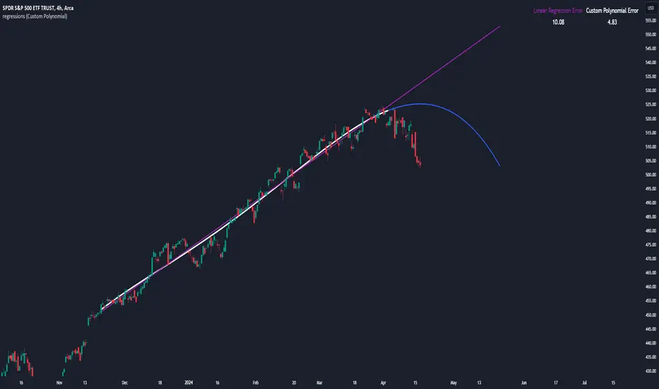
Predictivemodeling

regressionsLibrary "regressions"
This library computes least square regression models for polynomials of any form for a given data set of x and y values.
fit(X, y, reg_type, degrees)
Takes a list of X and y values and the degrees of the polynomial and returns a least square regression for the given polynomial on the dataset.
Parameters:
X (array) : (float ) X inputs for regression fit.
y (array) : (float ) y outputs for regression fit.
reg_type (string) : (string) The type of regression. If passing value for degrees use reg.type_custom
degrees (array) : (int ) The degrees of the polynomial which will be fit to the data. ex: passing array.from(0, 3) would be a polynomial of form c1x^0 + c2x^3 where c2 and c1 will be coefficients of the best fitting polynomial.
Returns: (regression) returns a regression with the best fitting coefficients for the selecected polynomial
regress(reg, x)
Regress one x input.
Parameters:
reg (regression) : (regression) The fitted regression which the y_pred will be calulated with.
x (float) : (float) The input value cooresponding to the y_pred.
Returns: (float) The best fit y value for the given x input and regression.
predict(reg, X)
Predict a new set of X values with a fitted regression. -1 is one bar ahead of the realtime
Parameters:
reg (regression) : (regression) The fitted regression which the y_pred will be calulated with.
X (array)
Returns: (float ) The best fit y values for the given x input and regression.
generate_points(reg, x, y, left_index, right_index)
Takes a regression object and creates chart points which can be used for plotting visuals like lines and labels.
Parameters:
reg (regression) : (regression) Regression which has been fitted to a data set.
x (array) : (float ) x values which coorispond to passed y values
y (array) : (float ) y values which coorispond to passed x values
left_index (int) : (int) The offset of the bar farthest to the realtime bar should be larger than left_index value.
right_index (int) : (int) The offset of the bar closest to the realtime bar should be less than right_index value.
Returns: (chart.point ) Returns an array of chart points
plot_reg(reg, x, y, left_index, right_index, curved, close, line_color, line_width)
Simple plotting function for regression for more custom plotting use generate_points() to create points then create your own plotting function.
Parameters:
reg (regression) : (regression) Regression which has been fitted to a data set.
x (array)
y (array)
left_index (int) : (int) The offset of the bar farthest to the realtime bar should be larger than left_index value.
right_index (int) : (int) The offset of the bar closest to the realtime bar should be less than right_index value.
curved (bool) : (bool) If the polyline is curved or not.
close (bool) : (bool) If true the polyline will be closed.
line_color (color) : (color) The color of the line.
line_width (int) : (int) The width of the line.
Returns: (polyline) The polyline for the regression.
series_to_list(src, left_index, right_index)
Convert a series to a list. Creates a list of all the cooresponding source values
from left_index to right_index. This should be called at the highest scope for consistency.
Parameters:
src (float) : (float ) The source the list will be comprised of.
left_index (int) : (float ) The left most bar (farthest back historical bar) which the cooresponding source value will be taken for.
right_index (int) : (float ) The right most bar closest to the realtime bar which the cooresponding source value will be taken for.
Returns: (float ) An array of size left_index-right_index
range_list(start, stop, step)
Creates an from the start value to the stop value.
Parameters:
start (int) : (float ) The true y values.
stop (int) : (float ) The predicted y values.
step (int) : (int) Positive integer. The spacing between the values. ex: start=1, stop=6, step=2:
Returns: (float ) An array of size stop-start
regression
Fields:
coeffs (array__float)
degrees (array__float)
type_linear (series__string)
type_quadratic (series__string)
type_cubic (series__string)
type_custom (series__string)
_squared_error (series__float)
X (array__float)
even_better_sinewave_mod
Description:
Even better sinewave was an indicator developed by John F. Ehlers (see Cycle Analytics for Trader, pg. 159), in which improvement to cycle measurements completely relies on strong normalization of the waveform. The indicator aims to create an artificially predictive indicator by transferring the cyclic data swings into a sine wave. In this indicator, the modified is on the weighted moving average as a smoothing function, instead of using the super smoother, aim to be more adaptive, and the default length is set to 55 bars.
Sinewave
smoothing = (7*hp + 6*hp_1 + 5*hp_2+ 4*hp_3 + 3*hp_4 + 2*hp5 + hp_6) /28
normalize = wave/sqrt(power)
Notes:
sinewave indicator crossing over -0.9 is considered to beginning of the cycle while crossing under 0.9 is considered as an end of the cycle
line color turns to green considered as a confirmation of an uptrend, while turns red as a confirmation of a downtrend
confidence of using indicator will be much in confirmation paired with another indicator such dynamic trendline e.g. moving average
as cited within Ehlers book Cycle Analytic for Traders, the indicator will be useful if the satisfied market cycle mode and the period of the dominant cycle must be estimated with reasonable accuracy
Other Example