Volume Conviction Index v1.0Volume Conviction Index V1 (VCI V1)
A robust, outlier-resistant volume oscillator designed to reveal real market participation and conviction behind price moves.
- Brief explainer -
v1.0 : Added a median line to show the movement and ultimate conviction of current price waves irrespective of current conviction. conviction can be extremely low (below zero line), yet price can be pumping, which shows the end of the current trend may be exhausting. divergence happens with this indicator is VERY FAST when tuned into it.
Core features:
• Median + MAD-based Z-score on volume (ignores extreme spikes/noise)
• Weighted blend: 60% robust deviation + 40% directional conviction (recent change % + relative volume %)
• Aggressive low-TF filter: optional rolling median line around zero to slice through 1min/3min chop
• Positive bars (teal) = unusual upward participation / conviction
• Negative bars (orange) = unusual weakness or drying volume
Use cases:
• Confirm breakouts, reversals, or exhaustion (e.g., spike on neckline breach)
• Filter false moves in low-liquidity or noisy periods
• Pair with Median Anchor Oscillator (MAO), Real Deviation Strength (RDS), and Anchor Pulse Wave (APW) for full conviction suite
V1 is raw and minimal — no signals, labels, or alerts yet. Feedback welcome for V2!
Companion suite:
• Median Anchor Oscillator
• Real Deviation Strength (RDS)
• Anchor Pulse Wave
© RU55IANROUL3TT3
Outlier

Moment-Based Adaptive DetectionMBAD (Moment-Based Adaptive Detection) : a method applicable to a wide range of purposes, like outlier or novelty detection, that requires building a sensible interval/set of thresholds. Unlike other methods that are static and rely on optimizations that inevitably lead to underfitting/overfitting, it dynamically adapts to your data distribution without any optimizations, MLE, or stuff, and provides a set of data-driven adaptive thresholds, based on closed-form solution with O(n) algo complexity.
1.5 years ago, when I was still living in Versailles at my friend's house not knowing what was gonna happen in my life tomorrow, I made a damn right decision not to give up on one idea and to actually R&D it and see what’s up. It allowed me to create this one.
The Method Explained
I’ve been wandering about z-values, why exactly 6 sigmas, why 95%? Who decided that? Why would you supersede your opinion on data? Based on what? Your ego?
Then I consciously noticed a couple of things:
1) In control theory & anomaly detection, the popular threshold is 3 sigmas (yet nobody can firmly say why xD). If your data is Laplace, 3 sigmas is not enough; you’re gonna catch too many values, so it needs a higher sigma.
2) Yet strangely, the normal distribution has kurtosis of 3, and 6 for Laplace.
3) Kurtosis is a standardized moment, a moment scaled by stdev, so it means "X amount of something measured in stdevs."
4) You generate synthetic data, you check on real data (market data in my case, I am a quant after all), and you see on both that:
lower extension = mean - standard deviation * kurtosis ≈ data minimum
upper extension = mean + standard deviation * kurtosis ≈ data maximum
Why not simply use max/min?
- Lower info gain: We're not using all info available in all data points to estimate max/min; we just pick the current higher and lower values. Lol, it’s the same as dropping exponential smoothing with alpha = 0 on stationary data & calling it a day.
You can’t update the estimates of min and max when new data arrives containing info about the matter. All you can do is just extend min and max horizontally, so you're not using new info arriving inside new data.
- Mixing order and non-order statistics is a bad idea; we're losing integrity and coherence. That's why I don't like the Hurst exponent btw (and yes, I came up with better metrics of my own).
- Max & min are not even true order statistics, unlike a percentile (finding which requires sorting, which requires multiple passes over your data). To find min or max, you just need to do one traversal over your data. Then with or without any weighting, 100th percentile will equal max. So unlike a weighted percentile, you can’t do weighted max. Then while you can always check max and min of a geometric shape, now try to calculate the 56th percentile of a pentagram hehe.
TL;DR max & min are rather topological characteristics of data, just as the difference between starting and ending points. Not much to do with statistics.
Now the second part of the ballet is to work with data asymmetry:
1) Skewness is also scaled by stdev -> so it must represent a shift from the data midrange measured in stdevs -> given asymmetric data, we can include this info in our models. Unlike kurtosis, skewness has a sign, so we add it to both thresholds:
lower extension = mean - standard deviation * kurtosis + standard deviation * skewness
upper extension = mean + standard deviation * kurtosis + standard deviation * skewness
2) Now our method will work with skewed data as well, omg, ain’t it cool?
3) Hold up, but what about 5th and 6th moments (hyperskewness & hyperkurtosis)? They should represent something meaningful as well.
4) Perhaps if extensions represent current estimated extremums, what goes beyond? Limits, beyond which we expect data not to be able to pass given the current underlying process generating the data?
When you extend this logic to higher-order moments, i.e., hyperskewness & hyperkurtosis (5th and 6th moments), they measure asymmetry and shape of distribution tails, not its core as previous moments -> makes no sense to mix 4th and 3rd moments (skewness and kurtosis) with 5th & 6th, so we get:
lower limit = mean - standard deviation * hyperkurtosis + standard deviation * hyperskewness
upper limit = mean + standard deviation * hyperkurtosis + standard deviation * hyperskewness
While extensions model your data’s natural extremums based on current info residing in the data without relying on order statistics, limits model your data's maximum possible and minimum possible values based on current info residing in your data. If a new data point trespasses limits, it means that a significant change in the data-generating process has happened, for sure, not probably—a confirmed structural break.
And finally we use time and volume weighting to include order & process intensity information in our model.
I can't stress it enough: despite the popularity of these non-weighted methods applied in mainstream open-access time series modeling, it doesn’t make ANY sense to use non-weighted calculations on time series data . Time = sequence, it matters. If you reverse your time series horizontally, your means, percentiles, whatever, will stay the same. Basically, your calculations will give the same results on different data. When you do it, you disregard the order of data that does have order naturally. Does it make any sense to you? It also concerns regressions applied on time series as well, because even despite the slope being opposite on your reversed data, the centroid (through which your regression line always comes through) will be the same. It also might concern Fourier (yes, you can do weighted Fourier) and even MA and AR models—might, because I ain’t researched it extensively yet.
I still can’t believe it’s nowhere online in open access. No chance I’m the first one who got it. It’s literally in front of everyone’s eyes for centuries—why no one tells about it?
How to use
That’s easy: can be applied to any, even non-stationary and/or heteroscedastic time series to automatically detect novelties, outliers, anomalies, structural breaks, etc. In terms of quant trading, you can try using extensions for mean reversion trades and limits for emergency exits, for example. The market-making application is kinda obvious as well.
The only parameter the model has is length, and it should NOT be optimized but picked consciously based on the process/system you’re applying it to and based on the task. However, this part is not about sharing info & an open-access instrument with the world. This is about using dem instruments to do actual business, and we can’t talk about it.
∞

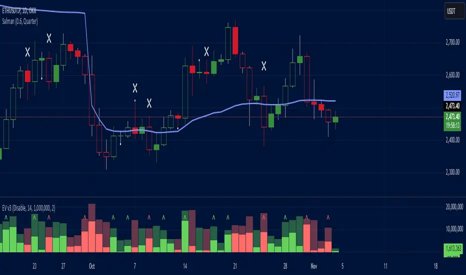
Effective Volume (ADV) v3Effective Volume (ADV) v3: Enhanced Accumulation/Distribution Analysis Tool
This indicator is an updated version of the original script by cI8DH, now upgraded to Pine Script v5 with added functionality, including the Volume Multiple feature. The tool is designed for analyzing Accumulation/Distribution (A/D) volume, referred to here as "Effective Volume," which represents the volume impact in alignment with price direction, providing insights into bullish or bearish trends through volume.
Accumulation/Distribution Volume Analysis : The script calculates and visualizes Effective Volume (ADV), helping traders assess volume strength in relation to price action. By factoring in bullish or bearish alignment, Effective Volume highlights points where volume strongly supports price movements.
Volume Multiple Feature for Volume Multiplication : The Volume Multiple setting (default value 2) allows you to set a multiplier to identify bars where Effective Volume exceeds the previous bar’s volume by a specified factor. This feature aids in pinpointing significant shifts in volume intensity, often associated with potential trend changes.
Customizable Aggregation Types : Users can choose from three volume aggregation types:
Simple - Standard SMA (Simple Moving Average) for averaging Effective Volume
Smoothed - RMA (Recursive Moving Average) for a less volatile, smoother line
Cumulative - Accumulated Effective Volume for ongoing trend analysis
Volume Divisor : The “Divide Vol by” setting (default 1 million) scales down the Effective Volume value for easier readability. This allows Effective Volume data to be aligned with the scale of the price chart.
Visualization Elements
Effective Volume Columns : The Effective Volume bar plot changes color based on volume direction:
Green Bars : Bullish Effective Volume (volume aligns with price movement upwards)
Red Bars : Bearish Effective Volume (volume aligns with price movement downwards)
Moving Average Lines :
Volume Moving Average - A gray line representing the moving average of total volume.
A/D Moving Average - A blue line showing the moving average of Accumulation/Distribution (A/D) Effective Volume.
High ADV Indicator : A “^” symbol appears on bars where the Effective Volume meets or exceeds the Volume Multiple threshold, highlighting bars with significant volume increase.
How to Use
Analyze Accumulation/Distribution Trends : Use Effective Volume to observe if bullish or bearish volume aligns with price direction, offering insights into the strength and sustainability of trends.
Identify Volume Multipliers with Volume Multiple : Adjust Volume Multiple to track when Effective Volume has notably increased, signaling potential shifts or strengthening trends.
Adjust Volume Display : Use the volume divisor setting to scale Effective Volume for clarity, especially when viewing alongside price data on higher timeframes.
With customizable parameters, this script provides a flexible, enhanced perspective on Effective Volume for traders analyzing volume-based trends and reversals.
Outlier changes alertAn indicator that calculates click (price change), percentage change, and Z-score changes while displaying outliers based on defined ranges.
Outlier Detection:
Mark outliers (for price, percentage, Z-score) based on user-defined thresholds. For example, any price movement exceeding a certain Z-score or percentage change could be marked as an outlier and displayed on chart.
Indicator Overview:
1. Click (Price Change):
Calculate the absolute price change from one period to another (e.g., from the current closing price to the previous closing price).
2. Percentage Change:
Calculate the percentage price change over a specific period, showing how much the price has changed in relative terms compared to the previous price.
3. Z-Score:
Compute the Z-score to standardize the price change relative to its historical average and standard deviation. The Z-score helps in detecting whether a price movement is an outlier or falls within a normal range of volatility.

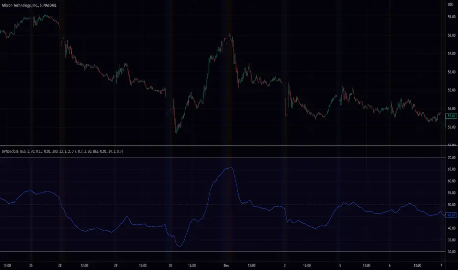
Band Pass Normalized Suite (BPNS)Outlier-Free Normalization and Band Pass Filtering
We present a technique for normalizing and filtering a given time series, source, in order to improve its stationarity and enhance its features. The technique includes two stages: outlier-free normalization and band pass filtering.
Outlier-Free Normalization:
In order to normalize source and reduce the impact of outliers, we first smooth the time series using an exponential moving average with a smoothing factor of alpha. The smoothed time series is then normalized by subtracting the minimum value within a given lookback period, dev_lookback, and dividing the result by the range (maximum - minimum) within the same lookback period. Outliers are detected and excluded from the normalization process by identifying values that are more than outlier_level standard deviations away from the exponentially smoothed average.
Band Pass Filtering:
After normalization, the time series is passed through a band pass filter to remove low and high frequency components. The specifics of the band pass filter implementation are not provided.
Code snippet:
bes(float source = close, float alpha = 0.7) =>
var float smoothed = na
smoothed := na(smoothed) ? source : alpha * source + (1 - alpha) * nz(smoothed )
max(source, outlier_level, dev_lookback)=>
var float max = na
src = array.new()
stdev = math.abs((source - bes(source, 0.1))/ta.stdev(source, dev_lookback))
array.push(src, stdev < outlier_level ? source : -1.7976931348623157e+308)
max := math.max(nz(max ), array.get(src, 0))
min(source, outlier_level, dev_lookback) =>
var float min = na
src = array.new()
stdev = math.abs((source - bes(source, 0.1))/ta.stdev(source, dev_lookback))
array.push(src, stdev < outlier_level ? source : 1.7976931348623157e+308)
min := math.min(nz(min ), array.get(src, 0))
min_max(src, outlier_level, dev_lookback) =>
(src - min(src, outlier_level, dev_lookback))/(max(src, outlier_level, dev_lookback) - min(src, outlier_level, dev_lookback)) * 100
To apply the outlier-free normalization and band pass filter to a given time series, source, the min_max() function can be called with the desired values for outlier_level and dev_lookback as arguments. For example:
normalized_source = min_max(source, 2, 50)
This will apply the outlier-free normalization and band pass filter to source, using an outlier_level of 2 standard deviations and a lookback period of 50 data points for both the normalization and outlier detection steps. The resulting normalized and filtered time series will be stored in normalized_source.
It is important to note that the choice of values for outlier_level and dev_lookback will have a significant impact on the resulting normalized and filtered time series. These values should be chosen carefully based on the characteristics of the input time series and the desired properties of the normalized and filtered output.
In conclusion, the outlier-free normalization and band pass filtering technique presented here provides a useful tool for preprocessing time series data and improving its stationarity and feature content. The flexibility of the method, through the choice of outlier_level and dev_lookback values, allows it to be tailored to the specific characteristics of the input time series.
Outliers Detector with N-Sigma Confidence Intervals (TG fork)Display outliers in either value change, volume or volume change that significantly deviate from the past.
This uses the standard deviation calculation and the n-sigmas statistical rule of significance, with 2-sigma (a value of 2) signifying that the observed value is stronger than 95% of past values, and 3-sigma 98.5% of past values, and so on for higher sigma values.
Outliers in price action or in volume can indicate a strong support for the move, and hence potentially more moves in the same direction in the future. Inversely, an insignificant move is less likely to be supported. And of course the stronger, the more support.
This indicator also doubles as a standard volume indicator if volume is selected as the source, but with the option of highlighting outliers.
Bars below significance can be uncolored (gray) to unclutter the visuals.
Differently to almost all other similar indicators, the background highlighting is dynamical, so that all values will be highlighted differently, not just 2-sigma or 3-sigma, but also 4-sigma, 5-sigma, etc, with a different value of transparency.
The dynamical transparency value can be calculated in two ways: either statically proportionally to the n-sigma but capped at 10-sigma, or either as a ratio relative to the highest observed sigma value over the defined lookback period (default: 300).
If you like this indicator, which is an extension of previously published indicators, please give some love to the original authors:
* tvjvzl :
* vnhilton :
This extension, authored by Tartigradia, extends tvjvzl's indi, implements vnhilton's idea of highlighting the background, and go further by adding dynamical background highlighting for any value of sigma, add support for volume and volume change (VolumeDiff) as inputs, add option to uncolor insignificant bars, allow plotting in both directions and more.

Median Absolute Deviation Filtered SMA & BBMedian Absolute Deviation (MAD) is a robust measurement of variability and more resilient against outliers and small samples.
This experiment uses MAD as a means of filtering outliers from an SMA calculation. First we construct the equivalent of a Bollinger Band, but based on the median as the basis and a multiple( k ) of MAD as the outlier cutoff.
k can be set a number of ways. As a simple multiple (3 - very conservative / 2.5 - moderately conservative / 2 - poorly conservative). Alternatively MAD can be used as an estimator of standard deviation by using a multiple of 1.4826 (SD1 - 1.4826 / SD2 - 2.9652 / SD3 - 4.4478).
Once we have a cutoff range an SMA is calculated with the outliers filtered out. Additionally a Bollinger band can be output using the filtered SMA as the basis and a multiple of the MAD instead of SD for the bands.
