ConeCastConeCast is a forward-looking projection indicator that visualizes a future price range (or "cone") based on recent trend momentum and adaptive volatility. Unlike lagging bands or reactive channels, this tool plots a predictive zone 3–50 bars ahead, allowing traders to anticipate potential price behavior rather than merely react to it.
How It Works
The core of ConeCast is a dynamic trend-slope engine derived from a Linear Regression line fitted over a user-defined lookback window. The slope of this trend is projected forward, and the cone’s width adapts based on real-time market volatility. In calm markets, the cone is narrow and focused. In volatile regimes, it expands proportionally, using an ATR-based % of price to scale.
Key Features
📈 Predictive Cone Zone: Visualizes a forward range using trend slope × volatility width.
🔄 Auto-Adaptive Volatility Scaling: Expands or contracts based on market quiet/chaotic states.
📊 Regime Detection: Identifies Bull, Bear, or Neutral states using a tunable slope threshold.
🧭 Multi-Timeframe Compatible: Slope and volatility can be calculated from higher timeframes.
🔔 Smart Alerts: Detects price entering the cone, and signals trend regime changes in real time.
🖼️ Clean Visual Output: Optionally includes outer cones, trend-trail marker, and dashboard label.
How to Use It
Use on 15m–4H charts for best forward visibility.
Look for price entering the cone as a potential trend continuation setup.
Monitor regime changes and volatility expansion to filter choppy market zones.
Tune the slope sensitivity and ATR multiplier to match your symbol's behavior.
Use outer cones to anticipate aggressive swings and wick traps.
What Makes It Unique
ConeCast doesn’t follow price — it predicts a possible future price envelope using trend + volatility math, without relying on lagging indicators or repainting logic. It's a hybrid of regression-based forecasting and dynamic risk zoning, designed for swing traders, scalpers, and algo developers alike.
Limitations
ConeCast projects based on current trend and volatility — it does not "know" future price. Like all projection tools, accuracy depends on trend persistence and market conditions. Use this in combination with confirmation signals and risk management.
Forward

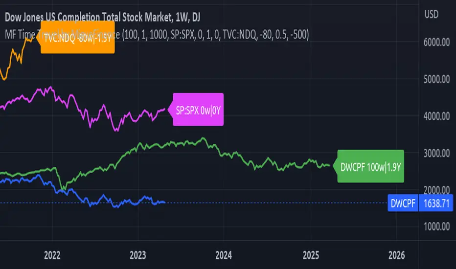
MF Time Travel (Delay or Forward Charts) by MigueFinanceThis indicator allows you to "Time Travel" aka. delay or advance (or forward) the on-screen chart/indicator as well as well as to do the same with other additional charts that can be configured in the settings.
This might be very useful when comparing with other (or the same) indicator in time, if you consider probably an incoming move based on another time performance.
About the Settings:
The moved in time charts can also be expanded or contracted, as well as they can be moved vertically (offset).
To Delay put positive values on the weeks settings, to Advance put Negative values on the same.
The Expansion or Contraction Factor is simply a multiplier of amplitude so you can multiply by number like 0.5, 2, etc
The Vertical Offset simply moves up and down the indicator.
The Labels will also tell you the number of weeks and years that were changed so as to have a reference, as well as the indicator being used.
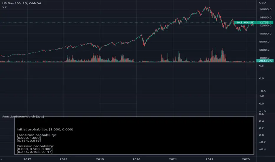
FunctionBaumWelchLibrary "FunctionBaumWelch"
Baum-Welch Algorithm, also known as Forward-Backward Algorithm, uses the well known EM algorithm
to find the maximum likelihood estimate of the parameters of a hidden Markov model given a set of observed
feature vectors.
---
### Function List:
> `forward (array pi, matrix a, matrix b, array obs)`
> `forward (array pi, matrix a, matrix b, array obs, bool scaling)`
> `backward (matrix a, matrix b, array obs)`
> `backward (matrix a, matrix b, array obs, array c)`
> `baumwelch (array observations, int nstates)`
> `baumwelch (array observations, array pi, matrix a, matrix b)`
---
### Reference:
> en.wikipedia.org
> github.com
> en.wikipedia.org
> www.rdocumentation.org
> www.rdocumentation.org
forward(pi, a, b, obs)
Computes forward probabilities for state `X` up to observation at time `k`, is defined as the
probability of observing sequence of observations `e_1 ... e_k` and that the state at time `k` is `X`.
Parameters:
pi (float ) : Initial probabilities.
a (matrix) : Transmissions, hidden transition matrix a or alpha = transition probability matrix of changing
states given a state matrix is size (M x M) where M is number of states.
b (matrix) : Emissions, matrix of observation probabilities b or beta = observation probabilities. Given
state matrix is size (M x O) where M is number of states and O is number of different
possible observations.
obs (int ) : List with actual state observation data.
Returns: - `matrix _alpha`: Forward probabilities. The probabilities are given on a logarithmic scale (natural logarithm). The first
dimension refers to the state and the second dimension to time.
forward(pi, a, b, obs, scaling)
Computes forward probabilities for state `X` up to observation at time `k`, is defined as the
probability of observing sequence of observations `e_1 ... e_k` and that the state at time `k` is `X`.
Parameters:
pi (float ) : Initial probabilities.
a (matrix) : Transmissions, hidden transition matrix a or alpha = transition probability matrix of changing
states given a state matrix is size (M x M) where M is number of states.
b (matrix) : Emissions, matrix of observation probabilities b or beta = observation probabilities. Given
state matrix is size (M x O) where M is number of states and O is number of different
possible observations.
obs (int ) : List with actual state observation data.
scaling (bool) : Normalize `alpha` scale.
Returns: - #### Tuple with:
> - `matrix _alpha`: Forward probabilities. The probabilities are given on a logarithmic scale (natural logarithm). The first
dimension refers to the state and the second dimension to time.
> - `array _c`: Array with normalization scale.
backward(a, b, obs)
Computes backward probabilities for state `X` and observation at time `k`, is defined as the probability of observing the sequence of observations `e_k+1, ... , e_n` under the condition that the state at time `k` is `X`.
Parameters:
a (matrix) : Transmissions, hidden transition matrix a or alpha = transition probability matrix of changing states
given a state matrix is size (M x M) where M is number of states
b (matrix) : Emissions, matrix of observation probabilities b or beta = observation probabilities. given state
matrix is size (M x O) where M is number of states and O is number of different possible observations
obs (int ) : Array with actual state observation data.
Returns: - `matrix _beta`: Backward probabilities. The probabilities are given on a logarithmic scale (natural logarithm). The first dimension refers to the state and the second dimension to time.
backward(a, b, obs, c)
Computes backward probabilities for state `X` and observation at time `k`, is defined as the probability of observing the sequence of observations `e_k+1, ... , e_n` under the condition that the state at time `k` is `X`.
Parameters:
a (matrix) : Transmissions, hidden transition matrix a or alpha = transition probability matrix of changing states
given a state matrix is size (M x M) where M is number of states
b (matrix) : Emissions, matrix of observation probabilities b or beta = observation probabilities. given state
matrix is size (M x O) where M is number of states and O is number of different possible observations
obs (int ) : Array with actual state observation data.
c (float ) : Array with Normalization scaling coefficients.
Returns: - `matrix _beta`: Backward probabilities. The probabilities are given on a logarithmic scale (natural logarithm). The first dimension refers to the state and the second dimension to time.
baumwelch(observations, nstates)
**(Random Initialization)** Baum–Welch algorithm is a special case of the expectation–maximization algorithm used to find the
unknown parameters of a hidden Markov model (HMM). It makes use of the forward-backward algorithm
to compute the statistics for the expectation step.
Parameters:
observations (int ) : List of observed states.
nstates (int)
Returns: - #### Tuple with:
> - `array _pi`: Initial probability distribution.
> - `matrix _a`: Transition probability matrix.
> - `matrix _b`: Emission probability matrix.
---
requires: `import RicardoSantos/WIPTensor/2 as Tensor`
baumwelch(observations, pi, a, b)
Baum–Welch algorithm is a special case of the expectation–maximization algorithm used to find the
unknown parameters of a hidden Markov model (HMM). It makes use of the forward-backward algorithm
to compute the statistics for the expectation step.
Parameters:
observations (int ) : List of observed states.
pi (float ) : Initial probaility distribution.
a (matrix) : Transmissions, hidden transition matrix a or alpha = transition probability matrix of changing states
given a state matrix is size (M x M) where M is number of states
b (matrix) : Emissions, matrix of observation probabilities b or beta = observation probabilities. given state
matrix is size (M x O) where M is number of states and O is number of different possible observations
Returns: - #### Tuple with:
> - `array _pi`: Initial probability distribution.
> - `matrix _a`: Transition probability matrix.
> - `matrix _b`: Emission probability matrix.
---
requires: `import RicardoSantos/WIPTensor/2 as Tensor`
Never Going Back AgainDraws lines for each of up to 500 prices that have never been revisited at the present moment in time, as time progresses these levels may or may not hodl.
Adaptation of "Never Look Back Price" originally described by Timothy Peterson in his research paper entitled "Why Bitcoin's Price Is Never Looking Back".
For more information see: static1.squarespace.com
