Vinicius Setup ATR
Description:
This script is a strategy based on the Supertrend indicator combined with volume analysis, candle strength, and RSI. Its goal is to identify potential entry points for buy and sell trades based on technical criteria, without promising profitability or guaranteed results.
Script Components:
Supertrend: Used as the main trend compass. When the trend is positive (direction = 1), buy signals are considered; when negative (direction = -1), sell signals are considered.
Volume: Entries are only validated if the volume is above the average of the last 20 candles, adjusted with a 1.2 multiplier.
Candle Body: The candle body must be larger than a certain percentage of the ATR, ensuring sufficient strength and volatility.
RSI: Used as a filter to avoid trades in extreme overbought or oversold zones.
Support and Resistance: Identified based on simple pivots (5 periods before and after).
Customizable Parameters:
ATR Length and Multiplier: Controls the sensitivity of the Supertrend.
RSI Period: Adjusts the relative strength filter.
Minimum Volume and Candle Body: Settings to validate entry signals.
Entry Conditions:
Buy: Positive trend + strong candle + high volume + RSI below 70.
Sell: Negative trend + strong candle + high volume + RSI above 30.
Exit Conditions:
The trade is closed upon the appearance of an opposite signal.
Notes:
This is a technical system with no profit guarantees.
It is recommended to test with realistic capital values and parameters suited to your risk management.
The script is not optimized for specific profitability, but rather to support study and the construction of setups with objective criteria.
Bandas e Canais

TASC 2025.05 Trading The Channel█ OVERVIEW
This script implements channel-based trading strategies based on the concepts explained by Perry J. Kaufman in the article "A Test Of Three Approaches: Trading The Channel" from the May 2025 edition of TASC's Traders' Tips . The script explores three distinct trading methods for equities and futures using information from a linear regression channel. Each rule set corresponds to different market behaviors, offering flexibility for trend-following, breakout, and mean-reversion trading styles.
█ CONCEPTS
Linear regression
Linear regression is a model that estimates the relationship between a dependent variable and one or more independent variables by fitting a straight line to the observed data. In the context of financial time series, traders often use linear regression to estimate trends in price movements over time.
The slope of the linear regression line indicates the strength and direction of the price trend. For example, a larger positive slope indicates a stronger upward trend, and a larger negative slope indicates the opposite. Traders can look for shifts in the direction of a linear regression slope to identify potential trend trading signals, and they can analyze the magnitude of the slope to support trading decisions.
One caveat to linear regression is that most financial time series data does not follow a straight line, meaning a regression line cannot perfectly describe the relationships between values. Prices typically fluctuate around a regression line to some degree. As such, analysts often project ranges above and below regression lines, creating channels to model the expected extent of the data's variability. This strategy constructs a channel based on the method used in Kaufman's article. It measures the maximum distances from points on the linear regression line to historical price values, then adds those distances and the current slope to the regression points.
Depending on the trading style, traders might look for prices to move outside an established channel for breakout signals, or they might look for price action to reach extremes within the channel for potential mean reversion opportunities.
█ STRATEGY CALCULATIONS
Primary trade rules
This strategy implements three distinct sets of rules for trend, breakout, and mean-reversion trades based on the methods Kaufman describes in his article:
Trade the trend (Rule 1) : Open new positions when the sign of the slope changes, indicating a potential trend reversal. Close short trades and enter a long trade when the slope changes from negative to positive, and do the opposite when the slope changes from positive to negative.
Trade channel breakouts (Rule 2) : Open new positions when prices cross outside the linear regression channel for the current sample. Close short trades and enter a long trade when the price moves above the channel, and do the opposite when the price moves below the channel.
Trade within the channel (Rule 3) : Open new positions based on price values within the channel's range. Close short trades and enter a long trade when the price is near the channel's low, within a specified percentage of the channel's range, and do the opposite when the price is near the channel's high. With this rule, users can also filter the trades based on the channel's slope. When the filter is active, long positions are allowed only when the slope is positive, and short positions are allowed only when it is negative.
Position sizing
Kaufman's strategy uses specific trade sizes for equities and futures markets:
For an equities symbol, the number of shares traded is $10,000 divided by the current price.
For a futures symbol, the number of contracts traded is based on a volatility-adjusted formula that divides $25,000 by the product of the 20-bar average true range and the instrument's point value.
By default, this script automatically uses these sizes for its trade simulation on equities and futures symbols and does not simulate trading on other symbols. However, users can control position sizes from the "Settings/Properties" tab and enable trade simulation on other symbol types by selecting the "Manual" option in the script's "Position sizing" input.
Stop-loss
This strategy includes the option to place an accompanying stop-loss order for each trade, which users can enable from the "SL %" input in the "Settings/Inputs" tab. When enabled, the strategy places a stop-loss order at a specified percentage distance from the closing price where the entry order occurs, allowing users to compare how the strategy performs with added loss protection.
█ USAGE
This strategy adapts its display logic for the three trading approaches based on the rule selected in the "Trade rule" input:
For all rules, the script plots the linear regression slope in a separate pane. The plot is color-coded to indicate whether the current slope is positive or negative.
When the selected rule is "Trade the trend", the script plots triangles in the separate pane to indicate when the slope's direction changes from positive to negative or vice versa. Additionally, it plots a color-coded SMA on the main chart pane, allowing visual comparison of the slope to directional changes in a moving average.
When the rule is "Trade channel breakouts" or "Trade within the channel", the script draws the current period's linear regression channel on the main chart pane, and it plots bands representing the history of the channel values from the specified start time onward.
When the rule is "Trade within the channel", the script plots overbought and oversold zones between the bands based on a user-specified percentage of the channel range to indicate the value ranges where new trades are allowed.
Users can customize the strategy's calculations with the following additional inputs in the "Settings/Inputs" tab:
Start date : Sets the date and time when the strategy begins simulating trades. The script marks the specified point on the chart with a gray vertical line. The plots for rules 2 and 3 display the bands and trading zones from this point onward.
Period : Specifies the number of bars in the linear regression channel calculation. The default is 40.
Linreg source : Specifies the source series from which to calculate the linear regression values. The default is "close".
Range source : Specifies whether the script uses the distances from the linear regression line to closing prices or high and low prices to determine the channel's upper and lower ranges for rules 2 and 3. The default is "close".
Zone % : The percentage of the channel's overall range to use for trading zones with rule 3. The default is 20, meaning the width of the upper and lower zones is 20% of the range.
SL% : If the checkbox is selected, the strategy adds a stop-loss to each trade at the specified percentage distance away from the closing price where the entry order occurs. The checkbox is deselected by default, and the default percentage value is 5.
Position sizing : Determines whether the strategy uses Kaufman's predefined trade sizes ("Auto") or allows user-defined sizes from the "Settings/Properties" tab ("Manual"). The default is "Auto".
Long trades only : If selected, the strategy does not allow short positions. It is deselected by default.
Trend filter : If selected, the strategy filters positions for rule 3 based on the linear regression slope, allowing long positions only when the slope is positive and short positions only when the slope is negative. It is deselected by default.
NOTE: Because of this strategy's trading rules, the simulated results for a specific symbol or channel configuration might have significantly fewer than 100 trades. For meaningful results, we recommend adjusting the start date and other parameters to achieve a reasonable number of closed trades for analysis.
Additionally, this strategy does not specify commission and slippage amounts by default, because these values can vary across market types. Therefore, we recommend setting realistic values for these properties in the "Cost simulation" section of the "Settings/Properties" tab.

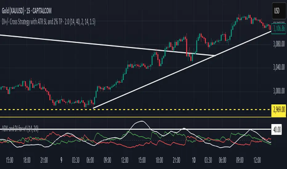
DI+/- Cross Strategy with ATR SL and 2% TPDI+/- Cross Strategy with ATR Stop Loss and 2% Take Profit
📝 Script Description for Publishing:
This strategy is based on the directional movement of the market using the Average Directional Index (ADX) components — DI+ and DI- — to generate entry signals, with clearly defined risk and reward targets using ATR-based Stop Loss and Fixed Percentage Take Profit.
🔍 How it works:
Buy Signal: When DI+ crosses above 40, signaling strong bullish momentum.
Sell Signal: When DI- crosses above 40, indicating strong bearish momentum.
Stop Loss: Dynamically calculated using ATR × 1.5, to account for market volatility.
Take Profit: Fixed at 2% above/below the entry price, for consistent reward targeting.
🧠 Why it’s useful:
Combines momentum breakout logic with volatility-based risk management.
Works well on trending assets, especially when combined with higher timeframe filters.
Clean BUY and SELL visual labels make it easy to interpret and backtest.
✅ Tips for Use:
Use on assets with clear trends (e.g., major forex pairs, trending stocks, crypto).
Best on 30m – 4H timeframes, but can be customized.
Consider combining with other filters (e.g., EMA trend direction or Bollinger Bands) for even better accuracy.
Donchian Breakout Strategy📈 Donchian Breakout Strategy (Inspired by Way of the Turtle)
This strategy is a modern adaptation of the legendary Turtle Trading system as taught in Way of the Turtle by Curtis Faith — re-engineered for the crypto market’s volatility, 24/7 nature, and frequent fakeouts.
⸻
🐢 Original Inspiration
The original Turtle system, created by Richard Dennis and William Eckhardt, used:
• Breakouts of Donchian Channels (20-day for entry, 10-day for exit)
• Volatility-based position sizing using ATR (N)
• Simple rules, big trend exposure, and pyramiding to grow winners
It was built for futures and commodities, trading daily bars, assuming stable trading hours and regulated markets.
⸻
🚀 What’s Different in This Strategy?
✅ Optimized for Crypto
• Adapts to constant volatility and price manipulation common in crypto
• Adds commission modeling for realistic results (0.045% default)
✅ Improved Entry Filtering
• Uses EMA filter to align with trend direction
• Adds RSI momentum check to avoid early or weak breakouts
• Optional volatility and volume filters to reduce false signals
✅ Smarter Exits
• ATR-based volatility stop loss, not just Donchian reversal
• Avoids pyramiding to reduce risk from sudden reversals
✅ Backtest-Friendly
• Default backtest window starts from 2025-01-01
• Fully configurable: long/short toggle, filter control, stop loss multiplier
⸻
🧪 Use Case
• Best on trending coins with strong directional moves
• Avoids chop via filters, preserving capital
• Can be tuned for aggressive or conservative setups with just a few tweaks

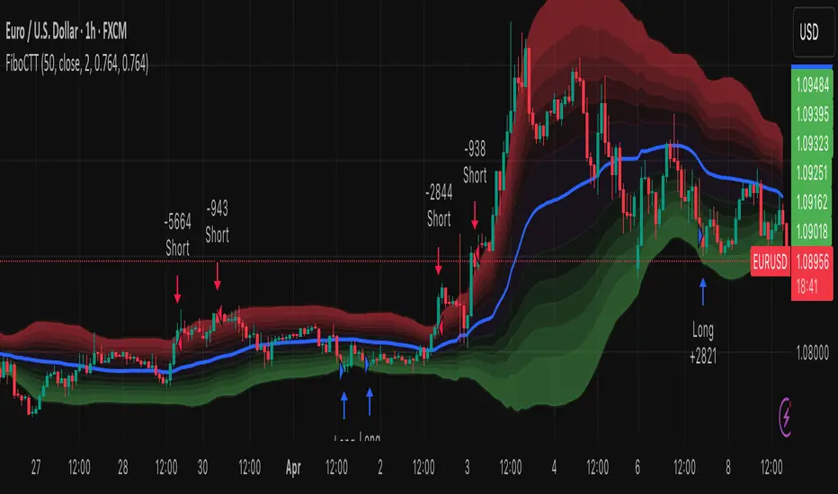
Fibonacci Counter-Trend TradingOverview:
The Fibonacci Counter-Trend Trading strategy is designed to capitalize on price reversals by utilizing Fibonacci levels calculated from the standard deviation of price movements. This strategy opens a sell order when the closing price crosses above a specified upper Fibonacci level and a buy order when the closing price crosses below a specified lower Fibonacci level. By leveraging the principles of Fibonacci retracement and volatility, this strategy aims to identify potential reversal points in the market.
How It Works:
Fibonacci Levels Calculation:
The strategy calculates upper and lower Fibonacci levels based on the standard deviation of the price over a specified moving average length. These levels are derived from the Fibonacci sequence, which is widely used in technical analysis to identify potential support and resistance levels.
The upper levels are calculated by adding specific Fibonacci ratios (0.236, 0.382, 0.5, 0.618, 0.764, and 1.0) multiplied by the standard deviation to the basis (the volume-weighted moving average).
The lower levels are calculated by subtracting the same Fibonacci ratios multiplied by the standard deviation from the basis.
Trade Entry Rules:
Sell Order: A sell order is triggered when the closing price crosses above the selected upper Fibonacci level. This indicates a potential reversal point where the price may start to decline.
Buy Order: A buy order is initiated when the closing price crosses below the selected lower Fibonacci level. This suggests a potential reversal point where the price may begin to rise.
Trade Management:
The strategy includes stop-losses based on the Fibonacci levels to protect against adverse price movements.
How to Use:
Users can customize the moving average length and the multiplier for the standard deviation to suit their trading preferences and market conditions.
The strategy can be applied to various financial instruments, including stocks, forex, and cryptocurrencies, making it versatile for different trading environments.
Pros:
The Fibonacci Counter-Trend Trading strategy combines the mathematical principles of the Fibonacci sequence with the statistical measure of standard deviation, providing a unique approach to identifying potential market reversals.
This strategy is particularly useful in volatile markets where price swings can lead to significant trading opportunities.
The use of Fibonacci levels can help traders identify key support and resistance areas, enhancing decision-making.
Cons:
The strategy may generate false signals in choppy or sideways markets, leading to potential losses if the price does not reverse as anticipated.
Relying solely on Fibonacci levels without considering other technical indicators or market conditions may result in missed opportunities or increased risk.
The effectiveness of the strategy can vary depending on the chosen parameters (e.g., moving average length and standard deviation multiplier), requiring users to spend time optimizing these settings for different market conditions.
As with any counter-trend strategy, there is a risk of significant drawdowns during strong trending markets, where the price continues to move in one direction without reversing.
By understanding the mechanics of the Fibonacci Counter-Trend Trading strategy, along with its pros and cons, traders can effectively implement it in their trading routines and potentially enhance their trading performance.
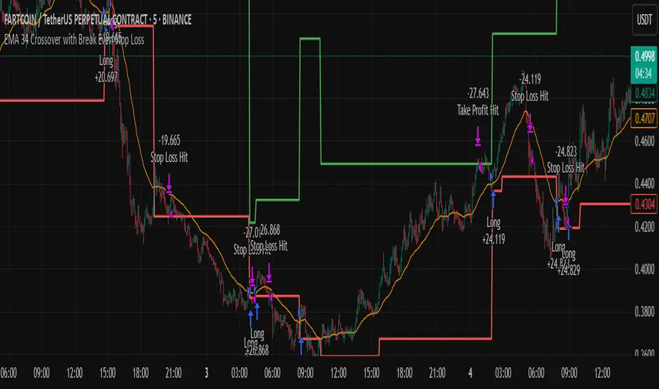
EMA 34 Crossover with Break Even Stop LossEMA 34 Crossover with Break Even Stop Loss Strategy
This trading strategy is based on the 34-period Exponential Moving Average (EMA) and aims to enter long positions when the price crosses above the EMA 34. The strategy is designed to manage risk effectively with a dynamic stop loss and take-profit mechanism.
Key Features:
EMA 34 Crossover:
The strategy generates a long entry signal when the closing price of the current bar crosses above the 34-period EMA, with the condition that the previous closing price was below the EMA. This crossover indicates a potential upward trend.
Risk Management:
Upon entering a trade, the strategy sets a stop loss at the low of the previous bar. This helps in controlling the downside risk.
A take profit level is set at a 10:1 risk-to-reward ratio, meaning the potential profit is ten times the amount risked on the trade.
Break-even Stop Loss:
As the price moves in favor of the trade and reaches a 3:1 risk-to-reward ratio, the strategy moves the stop loss to the entry price (break-even). This ensures that no loss will be incurred if the market reverses, effectively protecting profits.
Exit Conditions:
The strategy exits the trade when either the stop loss is hit (if the price drops below the stop loss level) or the take profit target is reached (if the price rises to the take profit level).
If the price reaches the break-even level (entry price), the stop loss is adjusted to lock in profits and prevent any loss.
Visualization:
The stop loss and take profit levels are plotted on the chart for easy visualization, helping traders track the status of their trade.
Trade Management Summary:
Long Entry: When price crosses above the 34-period EMA.
Stop Loss: Set to the low of the previous candle.
Take Profit: Set to a 10:1 risk-to-reward ratio.
Break-even: Stop loss is moved to entry price when a 3:1 risk-to-reward ratio is reached.
Exit: The trade is closed either when the stop loss or take profit levels are hit.
This strategy is designed to minimize losses by employing a dynamic stop loss and to maximize gains by setting a favorable risk-to-reward ratio, making it suitable for traders who prefer a structured, automated approach to risk management and trend-following.
Adaptive Fibonacci Pullback System -FibonacciFluxAdaptive Fibonacci Pullback System (AFPS) - FibonacciFlux
This work is licensed under a Attribution-NonCommercial-ShareAlike 4.0 International (CC BY-NC-SA 4.0). Original concepts by FibonacciFlux.
Abstract
The Adaptive Fibonacci Pullback System (AFPS) presents a sophisticated, institutional-grade algorithmic strategy engineered for high-probability trend pullback entries. Developed by FibonacciFlux, AFPS uniquely integrates a proprietary Multi-Fibonacci Supertrend engine (0.618, 1.618, 2.618 ratios) for harmonic volatility assessment, an Adaptive Moving Average (AMA) Channel providing dynamic market context, and a synergistic Multi-Timeframe (MTF) filter suite (RSI, MACD, Volume). This strategy transcends simple indicator combinations through its strict, multi-stage confluence validation logic. Historical simulations suggest that specific MTF filter configurations can yield exceptional performance metrics, potentially achieving Profit Factors exceeding 2.6 , indicative of institutional-level potential, while maintaining controlled risk under realistic trading parameters (managed equity risk, commission, slippage).
4 hourly MTF filtering
1. Introduction: Elevating Pullback Trading with Adaptive Confluence
Traditional pullback strategies often struggle with noise, false signals, and adapting to changing market dynamics. AFPS addresses these challenges by introducing a novel framework grounded in Fibonacci principles and adaptive logic. Instead of relying on static levels or single confirmations, AFPS seeks high-probability pullback entries within established trends by validating signals through a rigorous confluence of:
Harmonic Volatility Context: Understanding the trend's stability and potential turning points using the unique Multi-Fibonacci Supertrend.
Adaptive Market Structure: Assessing the prevailing trend regime via the AMA Channel.
Multi-Dimensional Confirmation: Filtering signals with lower-timeframe Momentum (RSI), Trend Alignment (MACD), and Market Conviction (Volume) using the MTF suite.
The objective is to achieve superior signal quality and adaptability, moving beyond conventional pullback methodologies.
2. Core Methodology: Synergistic Integration
AFPS's effectiveness stems from the engineered synergy between its core components:
2.1. Multi-Fibonacci Supertrend Engine: Utilizes specific Fibonacci ratios (0.618, 1.618, 2.618) applied to ATR, creating a multi-layered volatility envelope potentially resonant with market harmonics. The averaged and EMA-smoothed result (`smoothed_supertrend`) provides a robust, dynamic trend baseline and context filter.
// Key Components: Multi-Fibonacci Supertrend & Smoothing
average_supertrend = (supertrend1 + supertrend2 + supertrend3) / 3
smoothed_supertrend = ta.ema(average_supertrend, st_smooth_length)
2.2. Adaptive Moving Average (AMA) Channel: Provides dynamic market context. The `ama_midline` serves as a key filter in the entry logic, confirming the broader trend bias relative to adaptive price action. Extended Fibonacci levels derived from the channel width offer potential dynamic S/R zones.
// Key Component: AMA Midline
ama_midline = (ama_high_band + ama_low_band) / 2
2.3. Multi-Timeframe (MTF) Filter Suite: An optional but powerful validation layer (RSI, MACD, Volume) assessed on a lower timeframe. Acts as a **validation cascade** – signals must pass all enabled filters simultaneously.
2.4. High-Confluence Entry Logic: The core innovation. A pullback entry requires a specific sequence and validation:
Price interaction with `average_supertrend` and recovery above/below `smoothed_supertrend`.
Price confirmation relative to the `ama_midline`.
Simultaneous validation by all enabled MTF filters.
// Simplified Long Entry Logic Example (incorporates key elements)
long_entry_condition = enable_long_positions and
(low < average_supertrend and close > smoothed_supertrend) and // Pullback & Recovery
(close > ama_midline and close > ama_midline) and // AMA Confirmation
(rsi_filter_long_ok and macd_filter_long_ok and volume_filter_ok) // MTF Validation
This strict, multi-stage confluence significantly elevates signal quality compared to simpler pullback approaches.
1hourly filtering
3. Realistic Implementation and Performance Potential
AFPS is designed for practical application, incorporating realistic defaults and highlighting performance potential with crucial context:
3.1. Realistic Default Strategy Settings:
The script includes responsible default parameters:
strategy('Adaptive Fibonacci Pullback System - FibonacciFlux', shorttitle = "AFPS", ...,
initial_capital = 10000, // Accessible capital
default_qty_type = strategy.percent_of_equity, // Equity-based risk
default_qty_value = 4, // Default 4% equity risk per initial trade
commission_type = strategy.commission.percent,
commission_value = 0.03, // Realistic commission
slippage = 2, // Realistic slippage
pyramiding = 2 // Limited pyramiding allowed
)
Note: The default 4% risk (`default_qty_value = 4`) requires careful user assessment and adjustment based on individual risk tolerance.
3.2. Historical Performance Insights & Institutional Potential:
Backtesting provides insights into historical behavior under specific conditions (always specify Asset/Timeframe/Dates when sharing results):
Default Performance Example: With defaults, historical tests might show characteristics like Overall PF ~1.38, Max DD ~1.16%, with potential Long/Short performance variance (e.g., Long PF 1.6+, Short PF < 1).
Optimized MTF Filter Performance: Crucially, historical simulations demonstrate that meticulous configuration of the MTF filters (particularly RSI and potentially others depending on market) can significantly enhance performance. Under specific, optimized MTF filter settings combined with appropriate risk management (e.g., 7.5% risk), historical tests have indicated the potential to achieve **Profit Factors exceeding 2.6**, alongside controlled drawdowns (e.g., ~1.32%). This level of performance, if consistently achievable (which requires ongoing adaptation), aligns with metrics often sought in institutional trading environments.
Disclaimer Reminder: These results are strictly historical simulations. Past performance does not guarantee future results. Achieving high performance requires careful parameter tuning, adaptation to changing markets, and robust risk management.
3.3. Emphasizing Risk Management:
Effective use of AFPS mandates active risk management. Utilize the built-in Stop Loss, Take Profit, and Trailing Stop features. The `pyramiding = 2` setting requires particularly diligent oversight. Do not rely solely on default settings.
4. Conclusion: Advancing Trend Pullback Strategies
The Adaptive Fibonacci Pullback System (AFPS) offers a sophisticated, theoretically grounded, and highly adaptable framework for identifying and executing high-probability trend pullback trades. Its unique blend of Fibonacci resonance, adaptive context, and multi-dimensional MTF filtering represents a significant advancement over conventional methods. While requiring thoughtful implementation and risk management, AFPS provides discerning traders with a powerful tool potentially capable of achieving institutional-level performance characteristics under optimized conditions.
Acknowledgments
Developed by FibonacciFlux. Inspired by principles of Fibonacci analysis, adaptive averaging, and multi-timeframe confirmation techniques explored within the trading community.
Disclaimer
Trading involves substantial risk. AFPS is an analytical tool, not a guarantee of profit. Past performance is not indicative of future results. Market conditions change. Users are solely responsible for their decisions and risk management. Thorough testing is essential. Deploy at your own considered risk.

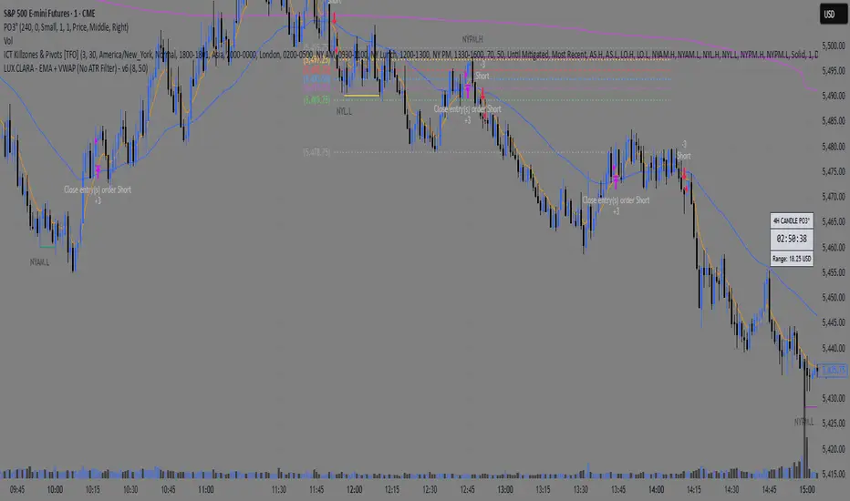
LUX CLARA - EMA + VWAP (No ATR Filter) - v6EMA STRAT SHOUT OUTOUTLIERSSSSS
Overview:
an intraday strategy built around two core principles:
Trend Confirmation using the 50 EMA (Exponential Moving Average) in relation to the VWAP (Volume-Weighted Average Price).
Entry Signals triggered by the 8 EMA crossing the 50 EMA in the direction of that confirmed trend.
Key Logic:
Bullish Trend if the 50 EMA is above VWAP. Only long entries are allowed when the 8 EMA crosses above the 50 EMA during that bullish phase.
Bearish Trend if the 50 EMA is below VWAP. Only short entries are allowed when the 8 EMA crosses below the 50 EMA during that bearish phase.
Intraday Focus: Trades are restricted to a user-defined session window (default 7:30 AM–11:30 AM), aligning entries/exits with peak intraday liquidity.
Exit Rule: Positions close automatically when the 8 EMA crosses back in the opposite direction of the entry.
Why It Works:
EMA + VWAP helps detect both immediate momentum (EMAs) and overall institutional bias (VWAP).
By confining trades to a set intraday window, the strategy aims to capture morning volatility while avoiding choppy afternoon or overnight sessions.
Customization:
Users can adjust EMA lengths, session times, or incorporate stops/targets for additional risk management.
It can be tested on various symbols and intraday timeframes to gauge performance and robustness.
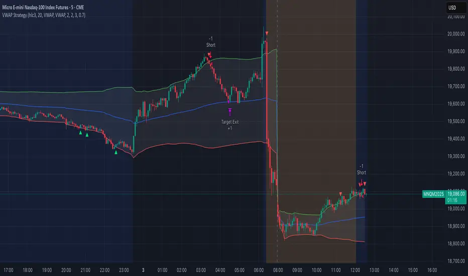
VWAP StrategyVWAP and volatility filters for structured intraday trades.
How the Strategy Works
1. VWAP Anchored to Session
VWAP is calculated from the start of each trading day.
Standard deviations are used to create bands above/below the VWAP.
2. Entry Triggers: Al Brooks H1/H2 and L1/L2
H1/H2 (Long Entry): Opens below 2nd lower deviation, closes above it.
L1/L2 (Short Entry): Opens above 2nd upper deviation, closes below it.
3. Volatility Filter (ATR)
Skips trades when deviation bands are too tight (< 3 ATRs).
4. Stop Loss
Based on the signal bar’s high/low ± stop buffer.
Longs: signalBarLow - stopBuffer
Shorts: signalBarHigh + stopBuffer
5. Take Profit / Exit Target
Exit logic is customizable per side:
VWAP, Deviation Band, or None
6. Safety Exit
Exits early if X consecutive bars go against the trade.
Longs: X red bars
Shorts: X green bars
Explanation of Strategy Inputs
- Stop Buffer: Distance from signal bar for stop-loss.
- Long/Short Exit Rule: VWAP, Deviation Band, or None
- Long/Short Target Deviation: Standard deviation for target exit.
- Enable Safety Exit: Toggle emergency exit.
- Opposing Bars: Number of opposing candles before safety exit.
- Allow Long/Short Trades: Enable or disable entry side.
- Show VWAP/Entry Bands: Toggle visual aids.
- Highlight Low Vol Zones: Orange shading for low volatility skips.
Tuning Tips
- Stop buffer: Use 1–5 points.
- Target deviation: Start with VWAP. In strong trends use 2nd deviation and turn off the counter-trend entry.
- Safety exit: 3 bars recommended.
- Disable short/long side to focus on one type of reversal.
Backtest Setup Suggestions
- initial_capital = 2000
- default_qty_value = 1 (fixed contracts or percent-of-equity)
Box Chart Overlay StrategyExploring the Box Chart Overlay Strategy with RSI & Bollinger Confirmation
The “Box Chart Overlay Strategy by BD” is a sophisticated TradingView strategy script written in Pine Script (version 5). It combines a box charting method with two widely used technical indicators—Relative Strength Index (RSI) and Bollinger Bands—to generate trade entries. In this article, we break down the strategy’s components, its logic, and how it visually represents trading signals on the chart.
1. Strategy Setup and User Inputs
Strategy Declaration
At the top of the script, the strategy is declared with key parameters:
Overlay: The indicator is plotted directly on the price chart.
Initial Capital & Position Sizing: It uses a simulated trading account with an initial capital of 10,000 and positions sized as a percentage of equity (10% by default).
Commission: A commission of 0.1% is factored into trades.
Input Parameters
The strategy is highly customizable. Users can adjust various inputs such as:
Box Settings:
Box Size (RSboxSize): Defines the size of each price “box.”
Box Options: Choose from three modes:
Standard: Boxes are calculated continuously from the start of the chart.
Anchored: The first box is fixed at a specified time and price.
Daily Reset: The boxes reset each day based on a defined session time.
Color Customizations:
Options to customize the appearance of boxes, borders, labels, and even repainting the candles based on the current price’s relation to box levels.
RSI Settings:
Length, overbought, and oversold levels are set to filter trades.
Bollinger Bands Settings:
Users can set the length of the moving average and the multiplier for standard deviation, which will be used to compute the upper and lower bands.
2. The Box Chart Mechanism
Box Construction
The core idea of a box chart is to group price movement into discrete blocks—or boxes—of a fixed size. In this strategy:
Standard Mode:
The script calculates boxes starting at a rounded price level. When the price moves sufficiently above or below the current box’s boundaries, a new box is drawn.
Anchored and Daily Reset Modes:
These modes allow traders to control where the box calculations begin or to reset them during a specific intraday session.
Visual Elements
Several custom functions handle the visual components:
drawBoxUp() and drawBoxDn():
These functions create boxes in bullish or bearish directions respectively, based on whether the price has exceeded the current box’s high or low.
drawLines() and drawLabels():
Lines are drawn to extend the current box levels, and labels are updated to display key levels or the “remainder” (the difference needed to trigger a new box).
Projected Boxes:
A “projected” box is drawn to indicate potential upcoming box levels, providing an additional visual cue about the price action.
3. Integrating RSI and Bollinger Bands for Trade Confirmation
RSI Integration
The strategy computes the RSI using a user-defined length. It then uses the following conditions to validate entries:
Long Trades (Box Up):
The strategy waits for the RSI to be at or below the oversold level before considering a long entry.
Short Trades (Box Down):
It requires the RSI to be at or above the overbought level before triggering a short entry.
Bollinger Bands Confirmation
In addition to the RSI filter:
For Long Entries:
The price must be at or below the lower Bollinger Band.
For Short Entries:
The price must be at or above the upper Bollinger Band.
By combining these filters with the box breakout logic, the strategy aims to enhance the quality of its trade signals.
4. Dynamic Trade Entries and Alerts
Box Logic and Entry Functions
Two key functions—BoxUpFunc() and BoxDownFunc()—handle the creation of new boxes and also check if trade conditions are met:
When a new box is drawn, the script evaluates if the RSI and Bollinger conditions align.
If conditions are satisfied, the script places an entry order:
Long Entry: Initiated when the price moves upward, RSI indicates oversold, and the price touches or falls below the lower Bollinger Band.
Short Entry: Triggered when the price falls downward, RSI signals overbought, and the price touches or exceeds the upper Bollinger Band.
Alerts
Built-in alert functions notify traders when a new box level is reached. Users can set custom alert messages to ensure they are aware of potential trade opportunities as soon as the conditions are met.
5. Visual Enhancements and Candle Repainting
The script also includes options for repainting candles based on their relation to the current box’s boundaries:
Above, Below, or Within the Box:
Candles are color-coded using user-defined colors, making it easier to visually assess where the price is in relation to the box levels.
Labels and Lines:
These continuously update to reflect current levels and provide an immediate visual reference for potential breakout points.
Conclusion
The Box Chart Overlay Strategy by BD is a multi-faceted approach that marries the traditional box chart technique with modern technical indicators—RSI and Bollinger Bands—to refine entry signals. By offering various customization options for box creation, visual styling, and confirmation criteria, the strategy allows traders to adapt it to different market conditions and personal trading styles. Whether you prefer a continuously running “Standard” mode or a more controlled “Anchored” or “Daily Reset” approach, this strategy provides a robust framework for integrating price action with momentum and volatility measures.

Qullamaggie [Modified] | FractalystWhat's the purpose of this strategy?
The strategy aims to identify high-probability breakout setups in trending markets, inspired by Kristjan "Qullamaggie" Kullamägi’s approach.
It focuses on capturing explosive price moves after periods of consolidation, using technical criteria like moving averages, breakouts, trailing stop-loss and momentum confirmation.
Ideal for swing traders seeking to ride strong trends while managing risk.
----
How does the strategy work?
The strategy follows a systematic process to capture high-momentum breakouts:
Pre-Breakout Criteria:
Prior Price Surge: Identifies stocks that have rallied 30-100%+ in recent month(s), signaling strong underlying momentum (per Qullamaggie’s volatility expansion principles).
Consolidation Phase: Looks for a tightening price range (e.g., flag, pennant, or tight base), indicating a potential "coiling" before continuation.
Trend Confirmation: Uses moving averages (e.g., 20/50/200 EMA) to ensure the stock is trading above key averages on the daily chart, confirming an uptrend.
Price Break: Enters when price clears the consolidation high with conviction.
Risk Management:
Initial Stop Loss: Placed below the consolidation low or a recent swing point to limit downside.
Break-Even Adjustment: Moves stop loss to breakeven once the trade reaches 1.5x risk-to-reward (RR), securing a "free trade" while letting winners run.
Trailing Stop (Unique Edge):
Market Structure Trailing: Instead of trailing via moving averages, the stop is dynamically adjusted using structural invalidation level. This adapts to price action, allowing the trade to stay open during volatile retracements while locking in gains as new structure forms.
Why This Matters: Most strategies use rigid trailing stops (e.g., below the 10EMA), which often exit prematurely in choppy markets. By trailing based on structure, this strategy avoids "noise" and captures larger trends, directly boosting overall returns.
----
What markets or timeframes is this suited for?
This is a long-only strategy designed for trending markets, and it performs best in:
Markets: Stocks (especially high-growth, liquid equities), cryptocurrencies (major pairs with strong volatility), commodities (e.g., oil, gold), and futures (index/commodity futures).
Timeframes: Primarily daily charts for swing trades (1-30 day holds), though weekly charts can help confirm broader trends.
Key Advantage: The TradingView script allows instant backtesting with adjustable parameters
You can:
- Test historical performance across multiple markets to identify which assets align best with the strategy.
- Optimize settings (e.g., trailing stop sensitivity, moving averages etc.) to match a market’s volatility profile.
Build a diversified portfolio by filtering for markets that show consistent profitability in backtests.
For example, you might discover cryptos require tighter trailing stops due to volatility, while stocks thrive with wider structural stops. The script automates this analysis, letting you to trade confidently.
----
What indicators or tools does the strategy use?
The strategy combines customizable technical tools with strict anti-lookahead safeguards:
Core Indicators:
Moving Averages: Adjustable periods (e.g., 20/50/200 EMA or SMA) and timeframes (daily/weekly) to confirm trend alignment. Users can test combinations (e.g., 10EMA vs. 20EMA) to optimize for specific markets.
Breakout Parameters:
Consolidation Length: Adjustable window to define the "tightness" of the pre-breakout pattern.
Entry Models: Flexible entry logics (Breakouts and fractals)
Anti-Lookahead Design:
All calculations (e.g., moving averages, consolidation ranges, volume averages) use only closed/confirmed data available at the time of the signal.
----
How do I manage risk with this strategy?
The strategy prioritizes customizable risk controls to align with your trading style and account size:
User-Defined Risk Inputs:
Risk Per Trade: Set a % of Equity (e.g., 1-2%) to determine position size. The strategy auto-calculates shares/contracts to match your selected risk per trade.
Flexibility: Choose between fixed risk or equity-based scaling.
The script adjusts position sizing dynamically based on your selection.
Pyramiding Feature:
Customizable Entries: Adjust the number of pyramiding trades allowed (e.g., 1-3 additional positions) in the strategy settings. Each new entry is triggered only if the prior trade hits its 1.5x RR target and the trend remains intact.
Risk-Scaled Additions: New positions use profits from prior trades, compounding gains without increasing initial risk.
Risk-Free Trade Mechanic:
Once a trade reaches 1.5x RR, the stop loss is moved to breakeven, eliminating downside risk.
The strategy then opens a new position (if pyramiding is enabled) using a portion of the locked-in profit. This "snowballs" winners while keeping total capital exposure stable.
Impact on Net Profit & Drawdown:
Net Profit Boost: Pyramiding lets you ride multi-leg trends aggressively. For example, a 100% runner could generate 2-3x more profit vs. a single-entry approach.
Controlled Drawdowns: Since new positions are funded by profits (not initial capital), max drawdown stays anchored to your original risk per trade (e.g., 1-2% of account). Even if later entries fail, the breakeven stop on prior trades protects overall equity.
Why This Works: Most strategies either over-leverage (increasing drawdowns) or exit too early. By recycling profits into new positions only after securing risk-free capital, this approach mimics hedge fund "scaling in" tactics while staying retail-trader friendly.
----
How does the strategy identify market structure for its trailing stoploss?
The strategy identifies market structure by utilizing an efficient logic with for loops to pinpoint the first swing candle that features a pivot of 2. This marks the beginning of the break of structure, where the market's previous trend or pattern is considered invalidated or changed.
----
What are the underlying calculations?
The underlying calculations involve:
Identifying Swing Points: The strategy looks for swing highs (marked with blue Xs) and swing lows (marked with red Xs). A swing high is identified when a candle's high is higher than the highs of the candles before and after it. Conversely, a swing low is when a candle's low is lower than the lows of the candles before and after it.
Break of Structure (BOS):
Bullish BOS: This occurs when the price breaks above the swing high level of the previous structure, indicating a potential shift to a bullish trend.
Bearish BOS: This happens when the price breaks below the swing low level of the previous structure, signaling a potential shift to a bearish trend.
Structural Liquidity and Invalidation:
Structural Liquidity: After a break of structure, liquidity levels are updated to the first swing high in a bullish BOS or the first swing low in a bearish BOS.
Structural Invalidation: If the price moves back to the level of the first swing low before the bullish BOS or the first swing high before the bearish BOS, it invalidates the break of structure, suggesting a potential reversal or continuation of the previous trend.
This method provides users with a technical approach to filter market regimes, offering an advantage by minimizing the risk of overfitting to historical data, which is often a concern with traditional indicators like moving averages.
By focusing on identifying pivotal swing points and the subsequent breaks of structure, the strategy maintains a balance between sensitivity to market changes and robustness against historical data anomalies, ensuring a more adaptable and potentially more reliable market analysis tool.
----
What entry criteria are used in this script?
The script uses two entry models for trading decisions: BreakOut and Fractal.
Underlying Calculations:
Breakout: The script records the most recent swing high by storing it in a variable. When the price closes above this recorded level, and all other predefined conditions are satisfied, the script triggers a breakout entry. This approach is considered conservative because it waits for the price to confirm a breakout above the previous high before entering a trade. As shown in the image, as soon as the price closes above the new candle (first tick), the long entry gets taken. The stop-loss is initially set and then moved to break-even once the price moves in favor of the trade.
Fractal: This method involves identifying a swing low with a period of 2, which means it looks for a low point where the price is lower than the two candles before and after it. Once this pattern is detected, the script executes the trade. This is an aggressive approach since it doesn't wait for further price confirmation. In the image, this is represented by the 'Fractal 2' label where the script identifies and acts on the swing low pattern.
----
What type of stop-loss identification method are used in this strategy?
This strategy employs two types of stop-loss methods: Initial Stop-loss and Trailing Stop-Loss.
Underlying Calculations:
Initial Stop-loss:
ATR Based: The strategy uses the Average True Range (ATR) to set an initial stop-loss, which helps in accounting for market volatility without predicting price direction.
Calculation:
- First, the True Range (TR) is calculated for each period, which is the greatest of:
- Current Period High - Current Period Low
- Absolute Value of Current Period High - Previous Period Close
- Absolute Value of Current Period Low - Previous Period Close
- The ATR is then the moving average of these TR values over a specified period, typically 14 periods by default. This ATR value can be used to set the stop-loss at a distance from the entry price that reflects the current market volatility.
Swing Low Based:
For this method, the stop-loss is set based on the most recent swing low identified in the market structure analysis. This approach uses the lowest point of the recent price action as a reference for setting the stop-loss.
Trailing Stop-Loss:
The strategy uses structural liquidity and structural invalidation levels across multiple timeframes to adjust the stop-loss once the trade is profitable. This method involves:
Detecting Structural Liquidity: After a break of structure, the liquidity levels are updated to the first swing high in a bullish scenario or the first swing low in a bearish scenario. These levels serve as potential areas where the price might find support or resistance, allowing the stop-loss to trail the price movement.
Detecting Structural Invalidation: If the price returns to the level of the first swing low before a bullish break of structure or the first swing high before a bearish break of structure, it suggests the trend might be reversing or invalidating, prompting the adjustment of the stop-loss to lock in profits or minimize losses.
By using these methods, the strategy dynamically adjusts the initial stop-loss based on market volatility, helping to protect against adverse price movements while allowing for enough room for trades to develop. The ATR-based stop-loss adapts to the current market conditions by considering the volatility, ensuring that the stop-loss is not too tight during volatile periods, which could lead to premature exits, nor too loose during calm markets, which might result in larger losses. Similarly, the swing low based stop-loss provides a logical exit point if the market structure changes unfavorably.
Each market behaves differently across various timeframes, and it is essential to test different parameters and optimizations to find out which trailing stop-loss method gives you the desired results and performance. This involves backtesting the strategy with different settings for the ATR period, the distance from the swing low, and how the trailing stop-loss reacts to structural liquidity and invalidation levels.
Through this process, you can tailor the strategy to perform optimally in different market environments, ensuring that the stop-loss mechanism supports the trade's longevity while safeguarding against significant drawdowns.
----
What type of break-even method is used in this strategy? What are the underlying calculations?
Moves the initial stop-loss to the entry price when the price reaches a certain RR ratio.
Calculation:
Break-even level = Entry Price + (Initial Risk * RR Ratio)
----
What tables are available in this script?
- Summary: Provides a general overview, displaying key performance parameters such as Net Profit, Profit Factor, Max Drawdown, Average Trade, Closed Trades and more.
Total Commission: Displays the cumulative commissions incurred from all trades executed within the selected backtesting window. This value is derived by summing the commission fees for each trade on your chart.
Average Commission: Represents the average commission per trade, calculated by dividing the Total Commission by the total number of closed trades. This metric is crucial for assessing the impact of trading costs on overall profitability.
Avg Trade: The sum of money gained or lost by the average trade generated by a strategy. Calculated by dividing the Net Profit by the overall number of closed trades. An important value since it must be large enough to cover the commission and slippage costs of trading the strategy and still bring a profit.
MaxDD: Displays the largest drawdown of losses, i.e., the maximum possible loss that the strategy could have incurred among all of the trades it has made. This value is calculated separately for every bar that the strategy spends with an open position.
Profit Factor: The amount of money a trading strategy made for every unit of money it lost (in the selected currency). This value is calculated by dividing gross profits by gross losses.
Avg RR: This is calculated by dividing the average winning trade by the average losing trade. This field is not a very meaningful value by itself because it does not take into account the ratio of the number of winning vs losing trades, and strategies can have different approaches to profitability. A strategy may trade at every possibility in order to capture many small profits, yet have an average losing trade greater than the average winning trade. The higher this value is, the better, but it should be considered together with the percentage of winning trades and the net profit.
Winrate: The percentage of winning trades generated by a strategy. Calculated by dividing the number of winning trades by the total number of closed trades generated by a strategy. Percent profitable is not a very reliable measure by itself. A strategy could have many small winning trades, making the percent profitable high with a small average winning trade, or a few big winning trades accounting for a low percent profitable and a big average winning trade. Most mean-reversion successful strategies have a percent profitability of 40-80% but are profitable due to risk management control.
BE Trades: Number of break-even trades, excluding commission/slippage.
Losing Trades: The total number of losing trades generated by the strategy.
Winning Trades: The total number of winning trades generated by the strategy.
Total Trades: Total number of taken traders visible your charts.
Net Profit: The overall profit or loss (in the selected currency) achieved by the trading strategy in the test period. The value is the sum of all values from the Profit column (on the List of Trades tab), taking into account the sign.
- Monthly: Displays performance data on a month-by-month basis, allowing users to analyze performance trends over each month and year.
- Weekly: Displays performance data on a week-by-week basis, helping users to understand weekly performance variations.
- UI Table: A user-friendly table that allows users to view and save the selected strategy parameters from user inputs. This table enables easy access to key settings and configurations, providing a straightforward solution for saving strategy parameters by simply taking a screenshot with Alt + S or ⌥ + S.
User-input styles and customizations:
Please note that all background colors in the style are disabled by default to enhance visualization.
How to Use This Strategy to Create a Profitable Edge and Systems?
Choose Your Strategy mode:
- Decide whether you are creating an investing strategy or a trading strategy.
Select a Market:
- Choose a one-sided market such as stocks, indices, or cryptocurrencies.
Historical Data:
- Ensure the historical data covers at least 10 years of price action for robust backtesting.
Timeframe Selection:
- Choose the timeframe you are comfortable trading with. It is strongly recommended to use a timeframe above 15 minutes to minimize the impact of commissions/slippage on your profits.
Set Commission and Slippage:
- Properly set the commission and slippage in the strategy properties according to your broker/prop firm specifications.
Parameter Optimization:
- Use trial and error to test different parameters until you find the performance results you are looking for in the summary table or, preferably, through deep backtesting using the strategy tester.
Trade Count:
- Ensure the number of trades is 200 or more; the higher, the better for statistical significance.
Positive Average Trade:
- Make sure the average trade is above zero.
(An important value since it must be large enough to cover the commission and slippage costs of trading the strategy and still bring a profit.)
Performance Metrics:
- Look for a high profit factor, and net profit with minimum drawdown.
- Ideally, aim for a drawdown under 20-30%, depending on your risk tolerance.
Refinement and Optimization:
- Try out different markets and timeframes.
- Continue working on refining your edge using the available filters and components to further optimize your strategy.
What Makes This Strategy Unique?
This strategy combines flexibility, smart risk management, and momentum focus in a way that’s rare and practical:
1. Adapts to Any Market Rhythm
Works on daily, weekly, or intraday charts without code changes.
Uses two entry types: classic breakouts (like trending stocks) or fractal patterns (to avoid false starts).
2. Smarter Stop-Loss System
No rigid rules: Stops adjust based on price structure (e.g., new “higher lows”), not fixed percentages.
Avoids whipsaws: Tightens stops only when the trend strengthens, not in choppy markets.
3. Safe Profit-Boosting Pyramiding
Adds new positions only after prior trades are risk-free (stops moved above breakeven).
Scales up using locked-in profits, not new capital, to grow gains safely.
4. Built-In Momentum Check
Tracks 1/3/6-month price growth to spotlight stocks with strong, lasting momentum.
Terms and Conditions | Disclaimer
Our charting tools are provided for informational and educational purposes only and should not be construed as financial, investment, or trading advice. They are not intended to forecast market movements or offer specific recommendations. Users should understand that past performance does not guarantee future results and should not base financial decisions solely on historical data.
Built-in components, features, and functionalities of our charting tools are the intellectual property of @Fractalyst Unauthorized use, reproduction, or distribution of these proprietary elements is prohibited.
- By continuing to use our charting tools, the user acknowledges and accepts the Terms and Conditions outlined in this legal disclaimer and agrees to respect our intellectual property rights and comply with all applicable laws and regulations.

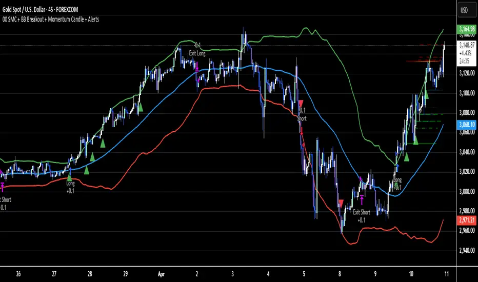
02 SMC + BB Breakout (Improved)This strategy combines Smart Money Concepts (SMC) with Bollinger Band breakouts to identify potential trading opportunities. SMC focuses on identifying key price levels and market structure shifts, while Bollinger Bands help pinpoint overbought/oversold conditions and potential breakout points. The strategy also incorporates higher timeframe trend confirmation to filter out trades that go against the prevailing trend.
Key Components:
Bollinger Bands:
Calculated using a Simple Moving Average (SMA) of the closing price and a standard deviation multiplier.
The strategy uses the upper and lower bands to identify potential breakout points.
The SMA (basis) acts as a centerline and potential support/resistance level.
The fill between the upper and lower bands can be toggled by the user.
Higher Timeframe Trend Confirmation:
The strategy allows for optional confirmation of the current trend using a higher timeframe (e.g., daily).
It calculates the SMA of the higher timeframe's closing prices.
A bullish trend is confirmed if the higher timeframe's closing price is above its SMA.
This helps filter out trades that go against the prevailing long-term trend.
Smart Money Concepts (SMC):
Order Blocks:
Simplified as recent price clusters, identified by the highest high and lowest low over a specified lookback period.
These levels are considered potential areas of support or resistance.
Liquidity Zones (Swing Highs/Lows):
Identified by recent swing highs and lows, indicating areas where liquidity may be present.
The Swing highs and lows are calculated based on user defined lookback periods.
Market Structure Shift (MSS):
Identifies potential changes in market structure.
A bullish MSS occurs when the closing price breaks above a previous swing high.
A bearish MSS occurs when the closing price breaks below a previous swing low.
The swing high and low values used for the MSS are calculated based on the user defined swing length.
Entry Conditions:
Long Entry:
The closing price crosses above the upper Bollinger Band.
If higher timeframe confirmation is enabled, the higher timeframe trend must be bullish.
A bullish MSS must have occurred.
Short Entry:
The closing price crosses below the lower Bollinger Band.
If higher timeframe confirmation is enabled, the higher timeframe trend must be bearish.
A bearish MSS must have occurred.
Exit Conditions:
Long Exit:
The closing price crosses below the Bollinger Band basis.
Or the Closing price falls below 99% of the order block low.
Short Exit:
The closing price crosses above the Bollinger Band basis.
Or the closing price rises above 101% of the order block high.
Position Sizing:
The strategy calculates the position size based on a fixed percentage (5%) of the strategy's equity.
This helps manage risk by limiting the potential loss per trade.
Visualizations:
Bollinger Bands (upper, lower, and basis) are plotted on the chart.
SMC elements (order blocks, swing highs/lows) are plotted as lines, with user-adjustable visibility.
Entry and exit signals are plotted as shapes on the chart.
The Bollinger band fill opacity is adjustable by the user.
Trading Logic:
The strategy aims to capitalize on Bollinger Band breakouts that are confirmed by SMC signals and higher timeframe trend. It looks for breakouts that align with potential market structure shifts and key price levels (order blocks, swing highs/lows). The higher timeframe filter helps avoid trades that go against the overall trend.
In essence, the strategy attempts to identify high-probability breakout trades by combining momentum (Bollinger Bands) with structural analysis (SMC) and trend confirmation.
Key User-Adjustable Parameters:
Bollinger Bands Length
Standard Deviation Multiplier
Higher Timeframe
Higher Timeframe Confirmation (on/off)
SMC Elements Visibility (on/off)
Order block lookback length.
Swing lookback length.
Bollinger band fill opacity.
This detailed description should provide a comprehensive understanding of the strategy's logic and components.
***DISCLAIMER: This strategy is for educational purposes only. It is not financial advice. Past performance is not indicative of future results. Use at your own risk. Always perform thorough backtesting and forward testing before using any strategy in live trading.***
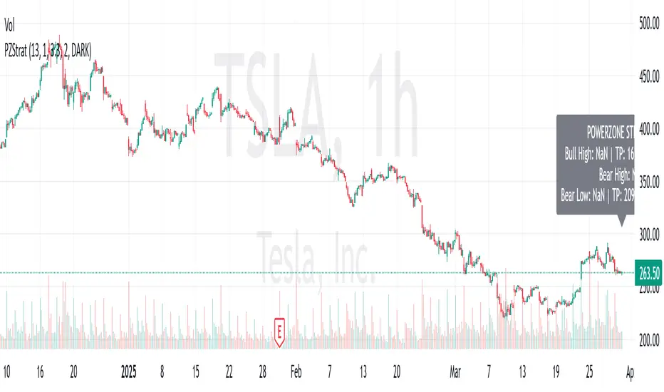
PowerZone Trading StrategyExplanation of the PowerZone Trading Strategy for Your Users
The PowerZone Trading Strategy is an automated trading strategy that detects strong price movements (called "PowerZones") and generates signals to enter a long (buy) or short (sell) position, complete with predefined take profit and stop loss levels. Here’s how it works, step by step:
1. What is a PowerZone?
A "PowerZone" (PZ) is a zone on the chart where the price has shown a significant and consistent movement over a specific number of candles (bars). There are two types:
Bullish PowerZone (Bullish PZ): Occurs when the price rises consistently over several candles after an initial bearish candle.
Bearish PowerZone (Bearish PZ): Occurs when the price falls consistently over several candles after an initial bullish candle.
The code analyzes:
A set number of candles (e.g., 5, adjustable via "Periods").
A minimum percentage move (adjustable via "Min % Move for PowerZone") to qualify as a strong zone.
Whether to use the full candle range (highs and lows) or just open/close prices (toggle with "Use Full Range ").
2. How Does It Detect PowerZones?
Bullish PowerZone:
Looks for an initial bearish candle (close below open).
Checks that the next candles (e.g., 5) are all bullish (close above open).
Ensures the total price movement exceeds the minimum percentage set.
Defines a range: from the high (or open) to the low of the initial candle.
Bearish PowerZone:
Looks for an initial bullish candle (close above open).
Checks that the next candles are all bearish (close below open).
Ensures the total price movement exceeds the minimum percentage.
Defines a range: from the high to the low (or close) of the initial candle.
These zones are drawn on the chart with lines: green or white for bullish, red or blue for bearish, depending on the color scheme ("DARK" or "BRIGHT").
3. When Does It Enter a Trade?
The strategy waits for a breakout from the PowerZone range to enter a trade:
Buy (Long): When the price breaks above the high of a Bullish PowerZone.
Sell (Short): When the price breaks below the low of a Bearish PowerZone.
The position size is set to 100% of available equity (adjustable in the code).
4. Take Profit and Stop Loss
Take Profit (TP): Calculated as a multiple (adjustable via "Take Profit Factor," default 1.5) of the PowerZone height. For example:
For a buy, TP = Entry price + (PZ height × 1.5).
For a sell, TP = Entry price - (PZ height × 1.5).
Stop Loss (SL): Calculated as a multiple (adjustable via "Stop Loss Factor," default 1.0) of the PZ height, placed below the range for buys or above for sells.
5. Visualization on the Chart
PowerZones are displayed with lines on the chart (you can hide them with "Show Bullish Channel" or "Show Bearish Channel").
An optional info panel ("Show Info Panel") displays key levels: PZ high and low, TP, and SL.
You can also enable brief documentation on the chart ("Show Documentation") explaining the basic rules.
6. Alerts
The code generates automatic alerts in TradingView:
For a bullish breakout: "Bullish PowerZone Breakout - LONG!"
For a bearish breakdown: "Bearish PowerZone Breakdown - SHORT!"
7. Customization
You can tweak:
The number of candles to detect a PZ ("Periods").
The minimum percentage move ("Min % Move").
Whether to use highs/lows or just open/close ("Use Full Range").
The TP and SL factors.
The color scheme and what elements to display on the chart.
Practical Example
Imagine you set "Periods = 5" and "Min % Move = 2%":
An initial bearish candle appears, followed by 5 consecutive bullish candles.
The total move exceeds 2%.
A Bullish PowerZone is drawn with a high and low.
If the price breaks above the high, you enter a long position with a TP 1.5 times the PZ height and an SL equal to the height below.
The system executes the trade and exits automatically at TP or SL.
Conclusion
This strategy is great for capturing strong price movements after consolidation or momentum zones. It’s automated, visual, and customizable, making it useful for both beginner and advanced traders. Try it out and adjust it to fit your trading style!
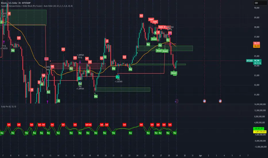
Supply & Demand Zones + Order Block (Pro Fusion) - Auto Order Strategy Title:
Smart Supply & Demand Zones + Order Block Auto Strategy with ScalpPro (Buy-Focused)
📄 Strategy Description:
This strategy combines the power of Supply & Demand Zone analysis, Order Block detection, and an enhanced Scalp Pro momentum filter, specifically designed for automated decision-making based on high-volume breakouts.
✅ Key Features:
Auto Entry (Buy Only) Based on Breakouts
Automatically enters a Buy position when the price breaks out of a valid demand zone, confirmed by EMA 50 trend and volume spike.
Order Block Logic
Identifies bullish and bearish order blocks using consecutive candle structures and significant price movement.
Dynamic Stop Loss & Trailing Stop
Implements a trailing stop once price moves in profit, along with static initial stop loss for risk management.
Clear Visual Labels & Alerts
Displays BUY/SELL, Demand/Supply, and Order Block labels directly on the chart. Alerts trigger on valid breakout signals.
Scalp Pro Momentum Filter (Optimized)
Uses a modified MACD-style momentum indicator to confirm trend strength and filter out weak signals.
Dual Keltner Channels Strategy [Eastgate3194]This strategy utilised 2 Keltner Channels to perform counter trade.
The strategy have 2 steps:
Long Position:
Step 1. Close price must cross under Outer Lower band of Keltner Channel.
Step 2. Close price cross over Inner Lower band of Keltner Channel.
Short Position:
Step 1. Close price must cross over Outer Upper band of Keltner Channel.
Step 2. Close price cross under Inner Upper band of Keltner Channel.

Keltner Channel StrategyOverview
The Keltner Channel Strategy is a powerful trend-following and mean-reversion system that leverages the Keltner Channels, EMA crossovers, and ATR-based stop-losses to optimize trade entries and exits. This strategy has proven to be highly effective, particularly when applied to Gold (XAUUSD) and other commodities with strong trend characteristics.
📈 How It Works
This strategy incorporates two trading approaches: 1️⃣ Keltner Channel Reversal Trades – Identifies overbought and oversold conditions when price touches the outer bands.
2️⃣ Trend Following Trades – Uses the 9 EMA & 21 EMA crossover, with confirmation from the 50 EMA, to enter trades in the direction of the trend.
🔍 Entry & Exit Criteria
📊 Keltner Channel Entries (Reversal Strategy)
✅ Long Entry: When the price crosses below the lower Keltner Band (potential reversal).
✅ Short Entry: When the price crosses above the upper Keltner Band (potential reversal).
⏳ Exit Conditions:
Long positions close when price crosses back above the mid-band (EMA-based).
Short positions close when price crosses back below the mid-band (EMA-based).
📈 Trend Following Entries (Momentum Strategy)
✅ Long Entry: When the 9 EMA crosses above the 21 EMA, and price is above the 50 EMA (bullish momentum).
✅ Short Entry: When the 9 EMA crosses below the 21 EMA, and price is below the 50 EMA (bearish momentum).
⏳ Exit Conditions:
Long positions close when the 9 EMA crosses back below the 21 EMA.
Short positions close when the 9 EMA crosses back above the 21 EMA.
📌 Risk Management & Profit Targeting
ATR-based Stop-Losses:
Long trades: Stop set at 1.5x ATR below entry price.
Short trades: Stop set at 1.5x ATR above entry price.
Take-Profit Levels:
Long trades: Profit target 2x ATR above entry price.
Short trades: Profit target 2x ATR below entry price.
🚀 Why Use This Strategy?
✅ Works exceptionally well on Gold (XAUUSD) due to high volatility.
✅ Combines reversal & trend strategies for improved adaptability.
✅ Uses ATR-based risk management for dynamic position sizing.
✅ Fully automated alerts for trade entries and exits.
🔔 Alerts
This script includes automated TradingView alerts for:
🔹 Keltner Band touches (Reversal signals).
🔹 EMA crossovers (Momentum trades).
🔹 Stop-loss & Take-profit activations.
📊 Ideal Markets & Timeframes
Best for: Gold (XAUUSD), NASDAQ (NQ), Crude Oil (CL), and trending assets.
Recommended Timeframes: 15m, 1H, 4H, Daily.
⚡️ How to Use
1️⃣ Add this script to your TradingView chart.
2️⃣ Select a 15m, 1H, or 4H timeframe for optimal results.
3️⃣ Enable alerts to receive trade notifications in real time.
4️⃣ Backtest and tweak ATR settings to fit your trading style.
🚀 Optimize your Gold trading with this Keltner Channel Strategy! Let me know how it performs for you. 💰📊

[3Commas] Turtle StrategyTurtle Strategy
🔷 What it does: This indicator implements a modernized version of the Turtle Trading Strategy, designed for trend-following and automated trading with webhook integration. It identifies breakout opportunities using Donchian channels, providing entry and exit signals.
Channel 1: Detects short-term breakouts using the highest highs and lowest lows over a set period (default 20).
Channel 2: Acts as a confirmation filter by applying an offset to the same period, reducing false signals.
Exit Channel: Functions as a dynamic stop-loss (wait for candle close), adjusting based on market structure (default 10 periods).
Additionally, traders can enable a fixed Take Profit level, ensuring a systematic approach to profit-taking.
🔷 Who is it for:
Trend Traders: Those looking to capture long-term market moves.
Bot Users: Traders seeking to automate entries and exits with bot integration.
Rule-Based Traders: Operators who prefer a structured, systematic trading approach.
🔷 How does it work: The strategy generates buy and sell signals using a dual-channel confirmation system.
Long Entry: A buy signal is generated when the close price crosses above the previous high of Channel 1 and is confirmed by Channel 2.
Short Entry: A sell signal occurs when the close price falls below the previous low of Channel 1, with confirmation from Channel 2.
Exit Management: The Exit Channel acts as a trailing stop, dynamically adjusting to price movements. To exit the trade, wait for a full bar close.
Optional Take Profit (%): Closes trades at a predefined %.
🔷 Why it’s unique:
Modern Adaptation: Updates the classic Turtle Trading Strategy, with the possibility of using a second channel with an offset to filter the signals.
Dynamic Risk Management: Utilizes a trailing Exit Channel to help protect gains as trades move favorably.
Bot Integration: Automates trade execution through direct JSON signal communication with your DCA Bots.
🔷 Considerations Before Using the Indicator:
Market & Timeframe: Best suited for trending markets; higher timeframes (e.g., H4, D1) are recommended to minimize noise.
Sideways Markets: In choppy conditions, breakouts may lead to false signals—consider using additional filters.
Backtesting & Demo Testing: It is crucial to thoroughly backtest the strategy and run it on a demo account before risking real capital.
Parameter Adjustments: Ensure that commissions, slippage, and position sizes are set accurately to reflect real trading conditions.
🔷 STRATEGY PROPERTIES
Symbol: BINANCE:ETHUSDT (Spot).
Timeframe: 4h.
Test Period: All historical data available.
Initial Capital: 10000 USDT.
Order Size per Trade: 1% of Capital, you can use a higher value e.g. 5%, be cautious that the Max Drawdown does not exceed 10%, as it would indicate a very risky trading approach.
Commission: Binance commission 0.1%, adjust according to the exchange being used, lower numbers will generate unrealistic results. By using low values e.g. 5%, it allows us to adapt over time and check the functioning of the strategy.
Slippage: 5 ticks, for pairs with low liquidity or very large orders, this number should be increased as the order may not be filled at the desired level.
Margin for Long and Short Positions: 100%.
Indicator Settings: Default Configuration.
Period Channel 1: 20.
Period Channel 2: 20.
Period Channel 2 Offset: 20.
Period Exit: 10.
Take Profit %: Disable.
Strategy: Long & Short.
🔷 STRATEGY RESULTS
⚠️Remember, past results do not guarantee future performance.
Net Profit: +516.87 USDT (+5.17%).
Max Drawdown: -100.28 USDT (-0.95%).
Total Closed Trades: 281.
Percent Profitable: 40.21%.
Profit Factor: 1.704.
Average Trade: +1.84 USDT (+1.80%).
Average # Bars in Trades: 29.
🔷 How to Use It:
🔸 Adjust Settings:
Select your asset and timeframe suited for trend trading.
Adjust the periods for Channel 1, Channel 2, and the Exit Channel to align with the asset’s historical behavior. You can visualize these channels by going to the Style tab and enabling them.
For example, if you set Channel 2 to 40 with an offset of 40, signals will take longer to appear but will aim for a more defined trend.
Experiment with different values, a possible exit configuration is using 20 as well. Compare the results and adjust accordingly.
Enable the Take Profit (%) option if needed.
🔸Results Review:
It is important to check the Max Drawdown. This value should ideally not exceed 10% of your capital. Consider adjusting the trade size to ensure this threshold is not surpassed.
Remember to include the correct values for commission and slippage according to the symbol and exchange where you are conducting the tests. Otherwise, the results will not be realistic.
If you are satisfied with the results, you may consider automating your trades. However, it is strongly recommended to use a small amount of capital or a demo account to test proper execution before committing real funds.
🔸Create alerts to trigger the DCA Bot:
Verify Messages: Ensure the message matches the one specified by the DCA Bot.
Multi-Pair Configuration: For multi-pair setups, enable the option to add the symbol in the correct format.
Signal Settings: Enable the option to receive long or short signals (Entry | TP | SL), copy and paste the messages for the DCA Bots configured.
Alert Setup:
When creating an alert, set the condition to the indicator and choose "alert() function call only".
Enter any desired Alert Name.
Open the Notifications tab, enable Webhook URL, and paste the Webhook URL.
For more details, refer to the section: "How to use TradingView Custom Signals".
Finalize Alerts: Click Create, you're done! Alerts will now be sent automatically in the correct format.
🔷 INDICATOR SETTINGS
Period Channel 1: Period of highs and lows to trigger signals
Period Channel 2: Period of highs and lows to filter signals
Offset: Move Channel 2 to the right x bars to try to filter out the favorable signals.
Period Exit: It is the period of the Donchian channel that is used as trailing for the exits.
Strategy: Order Type direction in which trades are executed.
Take Profit %: When activated, the entered value will be used as the Take Profit in percentage from the entry price level.
Use Custom Test Period: When enabled signals only works in the selected time window. If disabled it will use all historical data available on the chart.
Test Start and End: Once the Custom Test Period is enabled, here you select the start and end date that you want to analyze.
Check Messages: Check Messages: Enable this option to review the messages that will be sent to the bot.
Entry | TP | SL: Enable this options to send Buy Entry, Take Profit (TP), and Stop Loss (SL) signals.
Deal Entry and Deal Exit: Copy and paste the message for the deal start signal and close order at Market Price of the DCA Bot. This is the message that will be sent with the alert to the Bot, you must verify that it is the same as the bot so that it can process properly.
DCA Bot Multi-Pair: You must activate it if you want to use the signals in a DCA Bot Multi-pair in the text box you must enter (using the correct format) the symbol in which you are creating the alert, you can check the format of each symbol when you create the bot.
👨🏻💻💭 We hope this tool helps enhance your trading. Your feedback is invaluable, so feel free to share any suggestions for improvements or new features you'd like to see implemented.
__
The information and publications within the 3Commas TradingView account are not meant to be and do not constitute financial, investment, trading, or other types of advice or recommendations supplied or endorsed by 3Commas and any of the parties acting on behalf of 3Commas, including its employees, contractors, ambassadors, etc.

Bollinger Bands by Abu ElyasBollinger Bands with Adjustable Stop Loss (Long-Only)
This strategy uses a Bollinger Band breakout approach to enter long positions and incorporates an adjustable stop loss for risk management.
Below is an overview of the logic, parameters, and usage instructions.
1. Bollinger Bands Logic
Basis (Middle Band): A moving average (type selectable by the user) of the chosen source, typically the closing price.
Upper Band: The basis plus a specified number of standard deviations (user-defined multiplier).
Lower Band: The basis minus the same number of standard deviations.
2. Entry Triggers
The strategy enters a long position when the close price rises above the upper Bollinger Band , suggesting a potential bullish breakout.
This logic is only applied within a user-specified date range (adjustable in the strategy’s inputs).
3. Exit Triggers
1. Bollinger Band Exit:
If the close price drops below the lower Bollinger Band , the strategy closes the position, indicating a loss of bullish momentum.
2. Stop Loss Exit:
A default 8% stop loss is set, which automatically exits the trade if the close falls 8% below the entry price.
This stop-loss percentage is adjustable from the strategy’s settings, allowing users to tailor risk based on their preferences.
3. Date Range:
If the current bar is outside of the specified start/end dates, the strategy will also exit any open positions.
4. Position Sizing & Other Settings
1- Position Size:
By default, the script uses 100% of account equity for each trade.
2- Commissions & Slippage:
Commission is set to 0%, and slippage is set to 3 ticks.
3- Timeframe Handling:
You can select a custom timeframe or leave it blank to use the chart’s timeframe.
5. Customization
1. Bollinger Bands Parameters:
Length of the moving average, type of moving average (SMA, EMA, etc.), and the standard deviation multiplier can be adjusted.
2. Stop Loss (%)
The default stop loss of 8% can be changed in the script’s input settings to any percentage you prefer.
3. Date Filter:
Modify the start/end dates to control the historical period over which the strategy executes trades.
6. Notes & Best Practices
1- No Short Trades:
This is a long‐only strategy. It will either be in a long position or flat (no open position).
2- Risk Management:
An 8% stop loss may or may not align with your personal risk tolerance. Always adjust according to market conditions and your own trading style.
3- Market Gaps & Volatility:
In highly volatile markets, slippage or gaps can cause the actual exit price to be worse than the intended stop-loss level.
4- Test Thoroughly:
Backtest on different timeframes and market conditions. No single strategy works in all scenarios.
7. Disclaimer
Educational Use Only: This script is for informational and illustrative purposes and should not be considered financial advice.
No Guarantee of Profit: Past performance does not guarantee future results. Trading involves substantial risk, and it is possible to lose more than your initial investment.
Consult a Professional: Always consult a qualified financial advisor before making investment decisions.
Use this script as a foundation and personalize it based on your trading style, tolerance for drawdowns, and market conditions.

Dynamic Breakout Master by tradingbauhaus 🌟 Code Description:
This Pine Script implements a trading strategy called "Dynamic Breakout Master" 💥. The core idea of the strategy is to identify breakouts (price movements) at key support 💙 and resistance 🔴 levels, through a dynamic channel that adapts to the market’s conditions. Here's how it works:
🔧 Customizable Input Parameters:
🧭 Pivot Period: This defines the number of bars (candles) to the left and right used to detect pivots (highs and lows) that mark the support and resistance zones.
📊 Data Source: You can choose whether to use highs and lows or closes and opens of the candles to identify the pivots.
📏 Max Channel Width: Specifies the maximum width allowed for the support/resistance channel, expressed as a percentage over the last 300 bars.
💪 Minimum Pivot Strength: This defines the minimum number of pivots needed for a support or resistance level to be considered valid.
🏔 Max Support/Resistance Zones: Limits the number of key zones displayed on the chart.
📅 Lookback Period: Adjusts how many bars back the system should check to find and validate support and resistance levels.
🎨 Custom Colors: You can choose colors for the support, resistance, and in-channel zones.
📉 Moving Averages (MA): The strategy allows adding up to two moving averages (SMA or EMA) to assist in making trading decisions.
📊 Calculating Support/Resistance Levels:
The system uses an algorithm to identify pivots from prices and calculates dynamic support and resistance zones 🔒🔓.
The closer the pivots are and the stronger their influence, the more relevant the zone becomes for the strategy.
The dynamic channel is drawn on the chart, with a maximum width limit for these zones defined by the input parameter.
📈 Trading Logic:
🚀 Identifying Breakouts:
The strategy looks for when the price breaks (breakouts) a resistance or support level.
If the price breaks upward through the resistance level, a buy order 📈 is triggered.
If the price breaks downward through the support level, a sell order 📉 is triggered.
🔔 Alerts:
Resistance Break (ResBreak) and Support Break (SupBreak) alerts are configured to notify users when a significant breakout occurs.
💰 Commissions:
The strategy includes a commission (0.1%) to simulate transaction costs for each trade.
📊 Chart Visualization:
The support and resistance zones are displayed as colored rectangles:
🔴 Resistance (red) and
🔵 Support (blue).
Pivots of support and resistance can be labeled as P (for resistance) and V (for support).
Breakouts of support or resistance levels are marked with triangles that appear on the chart 🔺🔻.
📈 Trading Strategy:
If the price breaks upward through the resistance level, a long position (buy) 📈 is opened.
If the price breaks downward through the support level, a short position (sell) 📉 is opened.
🏆 Conclusion:
This script is a dynamic breakout strategy 💥 that allows traders to capture significant price movements when support or resistance channels break. The customizable parameters let users fine-tune the strategy according to their preferences, while the visual alerts on the chart make it easier to follow trading opportunities. The inclusion of moving averages and key price zones adds an extra layer of analysis to improve decision-making 💡.
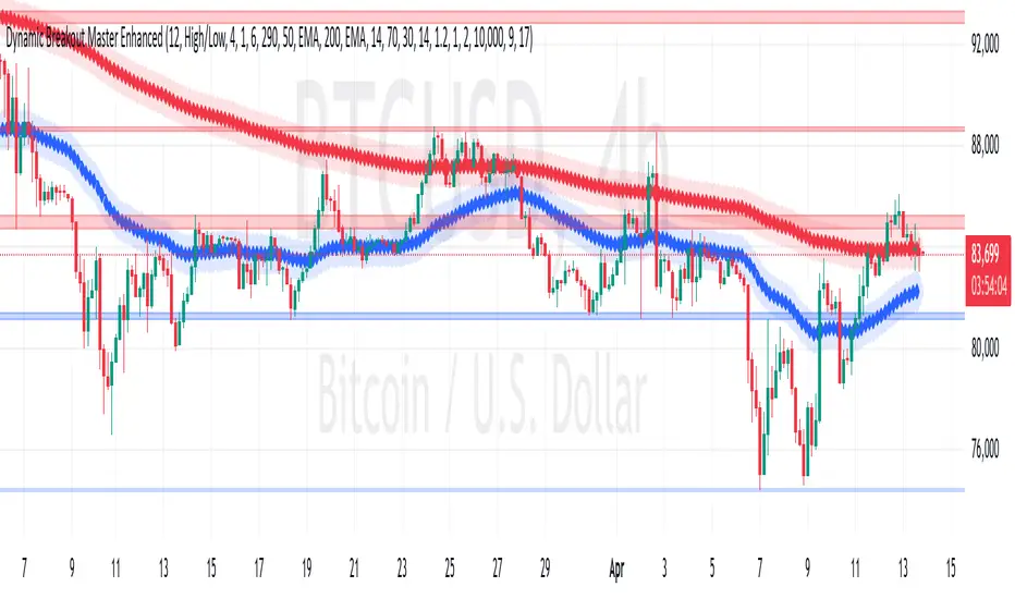
FVG Breakout Lite by tradingbauhausExplanation of "FVG Breakout Lite by tradingbauhaus"
This script is a trading strategy built for TradingView that helps you spot and trade "Fair Value Gaps" (FVGs)—price areas where the market moved quickly, leaving a gap that might act as support or resistance later. It’s designed to catch breakout opportunities when the price moves strongly in one direction, with extra filters to make trades more reliable. Here’s how it works and how you can use it:
What It Does
1. Finds Fair Value Gaps (FVGs):
A "Bullish FVG" happens when the price jumps up quickly, leaving a gap below where it didn’t trade much (e.g., today’s low is higher than the high from two bars ago).
A "Bearish FVG" is the opposite: the price drops fast, leaving a gap above (e.g., today’s high is lower than the low from two bars ago).
The script draws colored boxes on your chart to show these gaps: green for bullish, red for bearish.
2. Spots Breakouts:
It looks for "strong" FVGs by comparing them to a trend (based on the highest highs and lowest lows over a set period).
If a bullish gap forms above the recent highs, or a bearish gap below the recent lows, it’s marked as a breakout opportunity.
3. Adds a Volume Check:
Trades only happen if the market’s volume is higher than usual (e.g., 1.2x the average volume over the last 20 bars). This helps ensure the breakout has real momentum behind it.
4. Trades Automatically:
Long Trades (Buy): If a bullish breakout FVG forms and volume is high, it buys at the current price.
Short Trades (Sell): If a bearish breakout FVG forms with high volume, it sells short.
Each trade comes with a stop loss (to limit losses) and a take profit (to lock in gains), both adjustable by you.
5. Shows Mitigation Lines (Optional):
If you turn on "Display Mitigation Zones," it draws lines at the edge of each breakout FVG. These lines show where the price might return to "fill" the gap later, helping you see key levels.
6. Includes Webull Costs:
The script factors in real trading fees from Webull, like tiny SEC and FINRA fees for selling, and a daily margin cost if you’re borrowing money to trade. These don’t show up on the chart but affect the strategy’s performance in backtesting.
How to Use It
1. Add to Your Chart:
Copy the script into TradingView’s Pine Editor, click "Add to Chart," and it’ll start drawing FVGs and running the strategy.
2. Customize Settings:
Trend Period (Default: 25): How many bars it looks back to define the trend. Longer periods mean fewer but stronger signals.
Volume Lookback (Default: 20) & Volume Threshold (Default: 1.2): Adjust how it measures "high volume." Increase the threshold for stricter trades.
Stop Loss % (Default: 1.5%) & Take Profit % (Default: 3%): Set how much you’re willing to lose or aim to gain per trade.
Margin Rate % (Default: 8.74%): Webull’s rate for borrowing money—lower it if your account qualifies for a better rate.
Display Mitigation Zones (Default: On): Toggle this to see or hide the gap lines.
Colors: Change the green (bullish) and red (bearish) shades to suit your chart.
3. Backtest It:
Go to the "Strategy Tester" tab in TradingView to see how it performs on past data. It’ll show trades, profits, losses, and Webull fees included.
4. Watch It Work:
Green boxes mean bullish FVGs; red boxes mean bearish FVGs. If volume spikes and the price breaks out, you’ll see trades happen automatically.
What to Expect
Visuals: You’ll see colored boxes for FVGs and optional lines showing where they start. These help you spot key price zones even if you’re not trading.
Trades: It’s selective—only trades when FVGs align with a breakout and volume confirms it. Expect fewer trades but with higher potential.
Risk: The stop loss keeps losses in check, while the take profit aims for a 2:1 reward-to-risk ratio by default (3% gain vs. 1.5% loss).
Costs: Webull’s fees are small but baked into the results, so you’re seeing a realistic picture of profits.
Tips for Users
Test it on a small timeframe (like 5-minute charts) for day trading or a larger one (like daily) for swing trading.
Play with the volume threshold—if you get too few trades, lower it (e.g., 1.1); if too many, raise it (e.g., 1.5).
Watch how price reacts to the mitigation lines—they’re often support or resistance zones traders target.
This strategy is lightweight, focused, and built for traders who like breakouts with a bit of confirmation. It’s not foolproof (no strategy is!), but it gives you a clear way to trade FVGs with some smart filters.
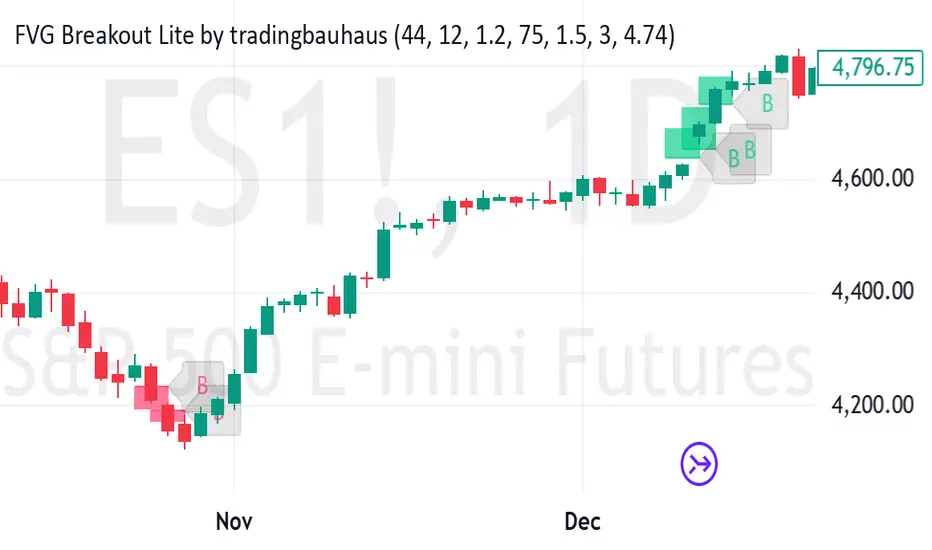
Slark Signal XtremeStrategy Description: Slark Signal Xtreme
The Slark Signal Xtreme is an innovative trading strategy designed to identify and capitalize on market opportunities by leveraging pivots, trend breakouts, and dynamic risk management. This strategy combines day-of-week and time filters with a ticks-based Stop Loss (SL) and Take Profit (TP) system, delivering customized signals and real-time alerts. Ideal for traders seeking a structured and highly customizable approach, Slark Signal Xtreme also incorporates advanced visual tools for efficient trade management.
Key Features:
Pivot- and Breakout-Based Signals: Utilizes pivot detection (highs/lows) combined with an ATR-based slope calculation to pinpoint trend changes and potential entry or exit points.
Dynamic Stop-Loss (SL) and Take-Profit (TP) Levels: Automatically calculates SL and TP based on the entry price and user-defined tick settings, adapting to volatility and optimizing risk management.
Time and Day Filters: Allows you to select specific days of the week and trading sessions during which signals are generated, avoiding low-liquidity periods or unwanted high volatility.
Customizable Risk Management: Lets you define the number of ticks for SL and TP, trading hours, initial capital, pyramiding, and commissions, tailoring the strategy to various risk profiles and assets.
Enhanced Visualization:
- SL and TP Boxes: Displays rectangular boxes on the chart indicating SL and TP levels, streamlining trade management.
- Candle Color Changes: Candles can be colored according to price position relative to pivot lines (bullish, bearish, or neutral).
- Session Highlight: Shades the chart background during the selected trading hours, providing immediate context on when the strategy is active.
Automated Alerts: Generates customizable alerts in TradingView whenever a buy or sell signal is triggered, detailing the timing, instrument, and SL/TP levels.
How the Strategy Works:
Technical Indicator Calculations:
- Pivot High/Low and Slope: Identifies price pivot points and calculates slope (based on ATR) to measure trend strength.
- Time and Day Filters: Signals only trigger within the specified days and hours, helping avoid undesirable market conditions.
Generating Buy and Sell Signals:
- Buy Signal (Long): Activated when price breaks above a downward pivot-based trendline or meets the condition for higher pivots.
- Sell Signal (Short): Activated when price breaks below an upward pivot-based trendline or meets the condition for lower pivots.
- Operation Conditions: Signals are only generated on selected days and during chosen trading hours, avoiding periods of low liquidity or excessive volatility.
Dynamic SL and TP Calculation:
- Stop-Loss (SL) and Take-Profit (TP): Determined by the entry price ± a user-defined number of ticks.
- SL and TP Visualization: Boxes are drawn on the chart from the entry price to SL/TP levels, enabling clear visual reference for trade management.
Order Execution and Alerts:
- Order Execution: When a signal is generated, Slark Signal Xtreme automatically opens a long or short position in TradingView’s backtesting environment.
- Alerts: Customizable alerts can be set up to provide real-time notifications (via TradingView or third-party integrations), offering essential details like instrument, time, SL/TP, etc.
Trade Management and Monitoring:
- Automatic Closure: Each trade is automatically closed upon reaching its SL or TP, ensuring disciplined risk control.
- Trade Summary: TradingView’s built-in reporting tools list all trades with cumulative results, simplifying performance evaluation.
Additional Visualization:
- Candle Coloring by Trend: Candles can be colored bullish, bearish, or neutral based on the pivot-driven trend detection.
- Operational Range Highlighting: The chart background is shaded during the permitted trading hours, clarifying when the strategy is active and enhancing visibility.
---
Strategy Properties (Important)
This backtest was conducted in TradingView under the following configuration:
Initial Capital: 1000 USD
Order Size: 10,000 contracts (adjust according to the traded asset)
Commission: 0.05 USD per order
Slippage: 1 tick
Pyramiding: 1 order
Price Verification for Limit Orders: 0 ticks
Recalculate on Every Tick & On Bar Close: Enabled
Bar Magnifier for Backtesting Precision: Enabled
These properties provide a realistic view of the strategy’s performance. However, default parameters may vary depending on each user or market:
Order Size: Should be calculated according to the asset traded and your desired risk level.
Commission and Slippage: Costs can vary by market and instrument; there is no universal default that guarantees realistic results.
All users are strongly recommended to adjust these properties within the script settings to match their own trading accounts and platforms, ensuring the most accurate backtest results.
---
Backtesting Results:
- Net Profit: +28.70
- Total Trades: 397
- Winning Trades: 138
- Win Rate: 34.76%
- Profit Factor: 1.07
- Sharpe Ratio: 1.25
- Sortino Ratio: 1.45
- Average Bars per Trade: 24
- Average Profit per Trade: 1.45
These numbers provide an overview of the strategy’s historical performance, demonstrating its potential for profitability given appropriate risk management.
---
Interpretation of Results:
- The strategy can be profitable despite a relatively modest win rate, thanks to a suitable risk-reward ratio.
- A profit factor of 1.07 indicates that total profits slightly exceed total losses.
- It is essential to monitor drawdown and ensure it aligns with your personal risk tolerance.
---
Risk Warning:
Trading leveraged financial instruments carries a high level of risk and may not be suitable for all investors. Before trading, carefully consider your investment objectives, experience level, and risk tolerance. Past performance does not guarantee future results. Always perform additional testing and adjust the strategy to your specific needs.
---
What Makes This Strategy Original?
Focus on Pivots and Time/Day Filters: Rather than purely relying on momentum indicators, Slark Signal Xtreme uses pivot-based signals and scheduling filters to capture higher-liquidity, directional market moves.
Dynamic Risk Management: Ticks-based SL/TP and customizable trading sessions enable precise adaptation to various markets and trading styles.
Advanced Visualization Tools: SL/TP boxes, candle coloring, and session highlights streamline market interpretation and facilitate real-time decision-making.
Seamless Alert Integration: Although native TradingView alerts are provided, it can be integrated with third-party messaging services (Telegram, Discord, etc.) for enhanced automation.
---
Additional Considerations
Continuous Testing and Optimization: Regularly backtest and fine-tune parameters (SL, TP, time filters, etc.) to accommodate changing market conditions.
Complementary Analysis: Combine this strategy with other technical or fundamental tools to confirm signals.
Rigorous Risk Management: Ensure SL/TP levels and position sizes conform to your overall risk management plan.
Updates and Support: Future updates and improvements may be released based on community feedback. For questions or suggestions, feel free to reach out.
---
Example Configuration
Assume you want to run Slark Signal Xtreme with these settings:
Trading Days: Monday to Friday
Trading Hours: 8:00 to 11:00 (exchange or broker time)
Stop Loss (SL) in Ticks: 100
Take Profit (TP) in Ticks: 300
SL/TP Box Extension: 20 bars
Initial Capital: 1000 USD
Risk per Trade: 1% of capital
Commissions & Slippage: 0.05 USD commission, 1 tick slippage
---
Conclusion
The Slark Signal Xtreme strategy delivers a robust and adaptable solution by merging pivots, time/day filters, flexible risk parameters, and advanced visualization. Its distinctive and customizable design makes it a powerful resource for traders aiming to diversify their methods and exploit trend breakouts under specific conditions. Fully compatible with TradingView, Slark Signal Xtreme can enhance your trading toolkit and foster a more systematic approach to your operations.
---
Final Disclaimer:
Financial markets are inherently volatile and pose significant risks. This strategy should be employed as part of a comprehensive trading plan and does not guarantee positive outcomes. Always consult a qualified financial advisor before making investment decisions. The use of Slark Signal Xtreme is solely at the user’s discretion, who must evaluate personal risk tolerance and financial objectives.
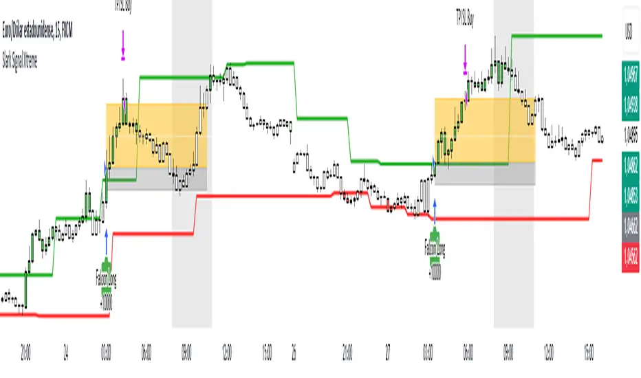
NSE Index Strategy with Entry/Exit MarkersExplanation of the Code
Trend Filter (200 SMA):
The line trendSMA = ta.sma(close, smaPeriod) calculates the 200‑period simple moving average. By trading only when the current price is above this SMA (inUptrend = close > trendSMA), we aim to trade in the direction of the dominant trend.
RSI Entry Signal:
The RSI is calculated with rsiValue = ta.rsi(close, rsiPeriod). The script checks for an RSI crossover above the oversold threshold using ta.crossover(rsiValue, rsiOversold). This helps capture a potential reversal from a minor pullback in an uptrend.
ATR-Based Exits:
ATR is computed by atrValue = ta.atr(atrPeriod) and is used to set the stop loss and take profit levels:
Stop Loss: stopLossPrice = close - atrMultiplier * atrValue
Take Profit: takeProfitPrice = close + atrMultiplier * atrValue
This dynamic approach allows the exit levels to adjust according to the current market volatility.
Risk and Money Management:
The strategy uses a fixed percentage of equity (10% by default) for each trade. The built‑in commission parameter helps simulate real-world trading costs.
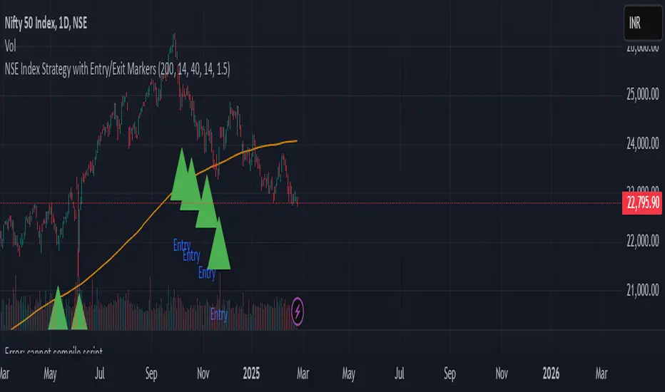
GM+For a Short Trade:
When a bullish candle (close > open) is larger than the previous candle and the MACD histogram for the past three bars is consecutively lower (suggesting weakening upward momentum), the script enters a short position.
For a Long Trade:
When a bearish candle (close < open) is larger (in body size) than the previous candle and the MACD histogram for the past three bars is consecutively higher (suggesting the downward move is losing strength), the script enters a long position.
Position Management:
There are no stop loss or take profit levels. The position is closed only when an opposite signal appears.
