Pattern Match & Forward Projection – Weekly (EN)
Overview
This indicator searches for recurring price patterns in weekly data and projects their average forward performance.
The logic is based on historical pattern repetition: it scans past price sequences similar to the most recent one, then aggregates their forward returns to estimate potential outcomes.
⚠️ Important: The indicator is designed for weekly timeframe only. Using it on daily or intraday charts will trigger an error message.
Settings (Inputs)
Pattern Settings
Pattern length (weeks): Number of weeks used to define the reference pattern.
Forward length (weeks): Number of weeks into the future to evaluate after each pattern match.
Lookback (weeks): Historical window to scan for past pattern matches.
Normalize by shape (z-score): If enabled, patterns are normalized by z-score, focusing on shape similarity rather than absolute values.
Distance threshold (Euclidean): Maximum allowed Euclidean distance between the reference pattern and historical candidates. Smaller values = stricter matching.
Min. required matches: Minimum number of valid matches needed for analysis.
Quality Filters
Min required Hit%: Minimum percentage of positive outcomes (upside forward returns) required for the pattern to be considered valid.
Return filter mode:
Either: absolute average return ≥ threshold
Long only: average return ≥ threshold
Short only: average return ≤ -threshold
Min avg return (%): Minimum average forward return threshold for validation.
Visual Options
Highlight historical matches (labels): Marks where in history similar patterns occurred.
Max match labels to draw: Caps the number of match markers shown to avoid clutter.
Draw average projection: Displays the average projected forward curve if conditions are met.
Show summary panel: Enables/disables the information panel.
Show weekly avg curve in panel: Adds a breakdown of average returns week by week.
Projection color: Choose the color of the projected forward curve.
What the Screen Shows
Summary Panel (top-left by default)
Total matches found in history
Matches with valid forward data
Average, minimum, and maximum distance (similarity measure)
Average forward return and Hit%
Distance threshold and normalization setting
Weekly average forward curve (if enabled)
Quality filter results (pass/fail)
Projection Curve (dotted line on price chart)
Drawn only if enough valid matches are found and filters are satisfied
Represents the average forward performance of historical matches, anchored at the current bar
Historical Match Labels (▲ markers)
Small arrows below past bars where similar patterns occurred
Tooltip: “Historical match”
Forecast Logic
The indicator does not predict the future in a deterministic way.
Instead, it relies on a pattern-matching algorithm:
The most recent N weeks (defined by Pattern length) are taken as the reference.
The algorithm scans the last Lookback (weeks) for segments with similar shape and magnitude.
Similarity is measured using Euclidean distance (optionally z-score normalized).
For each valid match, the subsequent Forward length weeks are collected.
These forward paths are averaged to generate a composite forward projection.
The summary panel reports whether the current setup passes the quality filters (Hit% and minimum average return).
Usage Notes
Best used as a contextual tool, not a standalone trading system.
Works only on weekly timeframe.
Quality filters help distinguish between noisy and statistically meaningful patterns.
A higher number of matches usually improves reliability, but very strict thresholds may reduce sample size.
📊 This tool is useful for traders who want to evaluate how similar historical setups have behaved and to visualize potential forward paths in a statistically aggregated way.
Pesquisar nos scripts por "algo"

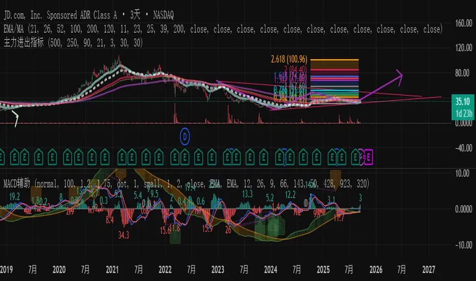
主力资金进出监控器Main Capital Flow Monitor-MEWINSIGHTMain Capital Flow Monitor Indicator
Indicator Description
This indicator utilizes a multi-cycle composite weighting algorithm to accurately capture the movement of main capital in and out of key price zones. The core logic is built upon three dimensions:
Multi-Cycle Pressure/Support System
Using triple timeframes (500-day/250-day/90-day) to calculate:
Long-term resistance lines (VAR1-3): Monitoring historical high resistance zones
Long-term support lines (VAR4-6): Identifying historical low support zones
EMA21 smoothing is applied to eliminate short-term fluctuations
Dynamic Capital Activity Engine
Proprietary VARD volatility algorithm:
VARD = EMA
Automatically amplifies volatility sensitivity by 10x when price approaches the safety margin (VARA×1.35), precisely capturing abnormal main capital movements
Capital Inflow Trigger Mechanism
Capital entry signals require simultaneous fulfillment of:
Price touching 30-day low zone (VARE)
Capital activity breaking recent peaks (VARF)
Weighted capital flow verified through triple EMA:
Capital Entry = EMA / 618
Visualization:
Green histogram: Continuous main capital inflow
Red histogram: Abnormal daily capital movement intensity
Column height intuitively displays capital strength
Application Scenarios:
Consecutive green columns → Main capital accumulation at bottom
Sudden expansion of red columns → Abnormal main capital rush
Continuous fluctuations near zero axis → Main capital washing phase
Core Value:
Provides 1-3 trading days early warning of main capital movements, suitable for:
Medium/long-term investors identifying main capital accumulation zones
Short-term traders capturing abnormal main capital breakouts
Risk control avoiding main capital distribution phases
Parameter Notes: Default parameters are optimized through historical A-share market backtesting. Users can adjust cycle parameters according to different market characteristics (suggest extending cycles by 20% for European/American markets).
Formula Features:
Multi-timeframe weighted synthesis technology
Dynamic sensitivity adjustment mechanism
Main capital activity intensity quantification
Early warning function for capital movements
Suitable Markets:
Stocks, futures, cryptocurrencies and other financial markets with obvious main capital characteristics.
指标名称:主力资金进出监控器
指标描述:
本指标通过多周期复合加权算法,精准捕捉主力资金在关键价格区域的进出动向。核心逻辑基于三大维度构建:
多周期压力/支撑体系
通过500日/250日/90日三重时间框架,分别计算:
长期压力线(VAR1-3):监控历史高位阻力区
长期支撑线(VAR4-6):识别历史低位承接区
采用EMA21平滑处理,消除短期波动干扰
动态资金活跃度引擎
独创VARD波动率算法:
当价格接近安全边际(VARA×1.35)时自动放大波动敏感度10倍,精准捕捉主力异动
资金进场触发机制
资金入场信号需同时满足:
价格触及30日最低区域(VARE)
资金活跃度突破近期峰值(VARF)
通过三重EMA验证的加权资金流:
资金入场 = EMA / 618
可视化呈现:
绿色柱状图:主力资金持续流入
红色柱状图:当日资金异动量级
柱体高度直观显示资金强度
使用场景:
绿色柱体连续出现 → 主力底部吸筹
红色柱体突然放大 → 主力异动抢筹
零轴附近持续波动 → 主力洗盘阶段
核心价值:
提前1-3个交易日预警主力资金动向,适用于:
中长线投资者识别主力建仓区间
短线交易者捕捉主力异动突破
风险控制规避主力出货阶段
参数说明:默认参数经A股历史数据回测优化,用户可根据不同市场特性调整周期参数(建议欧美市场延长周期20%)
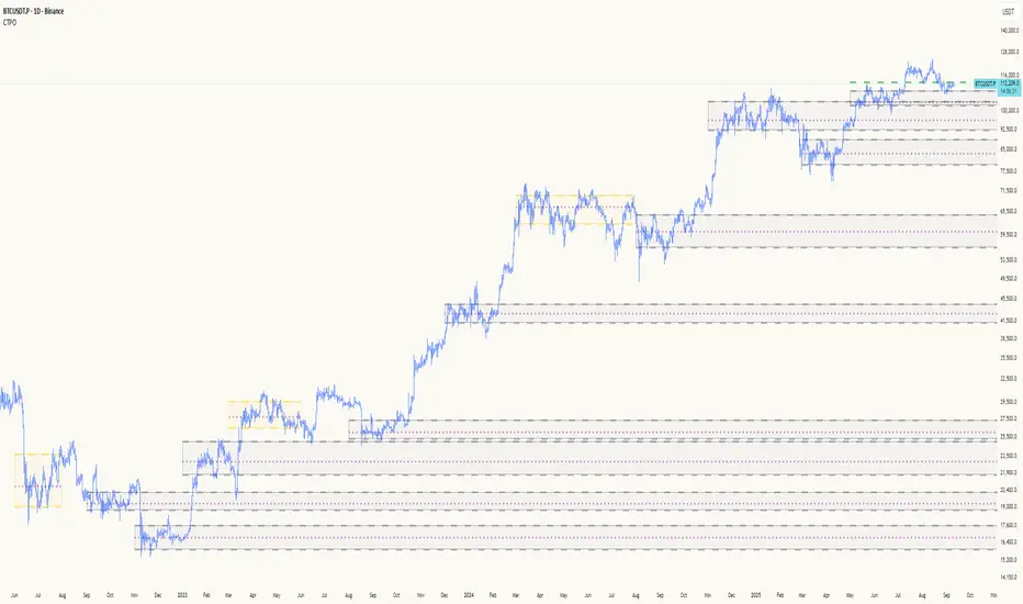
Composite Time ProfileComposite Time Profile Overlay (CTPO) - Market Profile Compositing Tool
Automatically composite multiple time periods to identify key areas of balance and market structure
What is the Composite Time Profile Overlay?
The Composite Time Profile Overlay (CTPO) is a Pine Script indicator that automatically composites multiple time periods to identify key areas of balance and market structure. It's designed for traders who use market profile concepts and need to quickly identify where price is likely to find support or resistance.
The indicator analyzes TPO (Time Price Opportunity) data across different timeframes and merges overlapping profiles to create composite levels that represent the most significant areas of balance. This helps you spot where institutional traders are likely to make decisions based on accumulated price action.
Why Use CTPO for Market Profile Trading?
Eliminate Manual Compositing Work
Instead of manually drawing and compositing profiles across different timeframes, CTPO does this automatically. You get instant access to composite levels without spending time analyzing each individual period.
Spot Areas of Balance Quickly
The indicator highlights the most significant areas of balance by compositing overlapping profiles. These areas often act as support and resistance levels because they represent where the most trading activity occurred across multiple time periods.
Focus on What Matters
Rather than getting lost in individual session profiles, CTPO shows you the composite levels that have been validated across multiple timeframes. This helps you focus on the levels that are most likely to hold.
How CTPO Works for Market Profile Traders
Automatic Profile Compositing
CTPO uses a proprietary algorithm that:
- Identifies period boundaries based on your selected timeframe (sessions, daily, weekly, monthly, or auto-detection)
- Calculates TPO profiles for each period using the C2M (Composite 2 Method) row sizing calculation
- Merges overlapping profiles using configurable overlap thresholds (default 50% overlap required)
- Updates composite levels as new price action develops in real-time
Key Levels for Market Profile Analysis
The indicator displays:
- Value Area High (VAH) and Value Area Low (VAL) levels calculated from composite TPO data
- Point of Control (POC) levels where most trading occurred across all composited periods
- Composite zones representing areas of balance with configurable transparency
- 1.618 Fibonacci extensions for breakout targets based on composite range
Multiple Timeframe Support
- Sessions: For intraday market profile analysis
- Daily: For swing trading with daily profiles
- Weekly: For position trading with weekly structure
- Monthly: For long-term market profile analysis
- Auto: Automatically selects timeframe based on your chart
Trading Applications for Market Profile Users
Support and Resistance Trading
Use composite levels as dynamic support and resistance zones. These levels often hold because they represent areas where significant trading decisions were made across multiple timeframes.
Breakout Trading
When composite levels break, they often lead to significant moves. The indicator calculates 1.618 Fibonacci extensions to give you clear targets for breakout trades.
Mean Reversion Strategies
Value Area levels represent the price range where most trading activity occurred. These levels often act as magnets, drawing price back when it moves too far from the mean.
Institutional Level Analysis
Composite levels represent areas where institutional traders have made significant decisions. These levels often hold more weight than traditional technical analysis levels because they're based on actual trading activity.
Key Features for Market Profile Traders
Smart Compositing Logic
- Automatic overlap detection using price range intersection algorithms
- Configurable overlap thresholds (minimum 50% overlap required for merging)
- Dead composite identification (profiles that become engulfed by newer composites)
- Real-time updates as new price action develops using barstate.islast optimization
Visual Customization
- Customizable colors for active, broken, and dead composites
- Adjustable transparency levels for each composite state
- Premium/Discount zone highlighting based on current price vs composite range
- TPO aggression coloring using TPO distribution analysis to identify buying/selling pressure
- Fibonacci level extensions with 1.618 target calculations based on composite range
Clean Chart Presentation
- Only shows the most relevant composite levels (maximum 10 active composites)
- Eliminates clutter from individual session profiles
- Focuses on areas of balance that matter most to current price action
Real-World Trading Examples
Day Trading with Session Composites
Use session-based composites to identify intraday areas of balance. The VAH and VAL levels often act as natural profit targets and stop-loss levels for scalping strategies.
Swing Trading with Daily Composites
Daily composites provide excellent swing trading levels. Look for price reactions at composite zones and use the 1.618 extensions for profit targets.
Position Trading with Weekly Composites
Weekly composites help identify major trend changes and long-term areas of balance. These levels often hold for months or even years.
Risk Management
Composite levels provide natural stop-loss levels. If a composite level breaks, it often signals a significant shift in market sentiment, making it an ideal place to exit losing positions.
Why Composite Levels Work
Composite levels work because they represent areas where significant trading decisions were made across multiple timeframes. When price returns to these levels, traders often remember the previous price action and make similar decisions, creating self-fulfilling prophecies.
The compositing process uses a proprietary algorithm that ensures only levels validated across multiple time periods are displayed. This means you're looking at levels that have proven their significance through actual market behavior, not just random technical levels.
Technical Foundation
The indicator uses TPO (Time Price Opportunity) data combined with price action analysis to identify areas of balance. The C2M row sizing method ensures accurate profile calculations, while the overlap detection algorithm (minimum 50% price range intersection) ensures only truly significant composites are displayed. The algorithm calculates row size based on ATR (Average True Range) divided by 10, then converts to tick size for precise level calculations.
How the Code Actually Works
1. Period Detection and ATR Calculation
The code first determines the appropriate timeframe based on your chart:
- 1m-5m charts: Session-based profiles
- 15m-2h charts: Daily profiles
- 4h charts: Weekly profiles
- 1D charts: Monthly profiles
For each period type, it calculates the number of bars needed for ATR calculation:
- Sessions: 540 minutes divided by chart timeframe
- Daily: 1440 minutes divided by chart timeframe
- Weekly: 7 days worth of minutes divided by chart timeframe
- Monthly: 30 days worth of minutes divided by chart timeframe
2. C2M Row Size Calculation
The code calculates True Range for each bar in the determined period:
- True Range = max(high-low, |high-prevClose|, |low-prevClose|)
- Averages all True Range values to get ATR
- Row Size = (ATR / 10) converted to tick size
- This ensures each TPO row represents a meaningful price movement
3. TPO Profile Generation
For each period, the code:
- Creates price levels from lowest to highest price in the range
- Each level is separated by the calculated row size
- Counts how many bars touch each price level (TPO count)
- Finds the level with highest count = Point of Control (POC)
- Calculates Value Area by expanding from POC until 68.27% of total TPO blocks are included
4. Overlap Detection Algorithm
When a new profile is created, the code checks if it overlaps with existing composites:
- Calculates overlap range = min(currentVAH, prevVAH) - max(currentVAL, prevVAL)
- Calculates current profile range = currentVAH - currentVAL
- Overlap percentage = (overlap range / current profile range) * 100
- If overlap >= 50%, profiles are merged into a composite
5. Composite Merging Logic
When profiles overlap, the code creates a new composite by:
- Taking the earliest start bar and latest end bar
- Using the wider VAH/VAL range (max of both profiles)
- Keeping the POC from the profile with more TPO blocks
- Marking the composite as "active" until price breaks through
6. Real-Time Updates
The code uses barstate.islast to optimize performance:
- Only recalculates on the last bar of each period
- Updates active composite with live price action if enabled
- Cleans up old composites to prevent memory issues
- Redraws all visual elements from scratch each bar
7. Visual Rendering System
The code uses arrays to manage drawing objects:
- Clears all lines/boxes arrays on every bar
- Iterates through composites array to redraw everything
- Uses different colors for active, broken, and dead composites
- Calculates 1.618 Fibonacci extensions for broken composites
Getting Started with CTPO
Step 1: Choose Your Timeframe
Select the period type that matches your trading style:
- Use "Sessions" for day trading
- Use "Daily" for swing trading
- Use "Weekly" for position trading
- Use "Auto" to let the indicator choose based on your chart timeframe
Step 2: Customize the Display
Adjust colors, transparency, and display options to match your charting preferences. The indicator offers extensive customization options to ensure it fits seamlessly into your existing analysis.
Step 3: Identify Key Levels
Look for:
- Composite zones (blue boxes) - major areas of balance
- VAH/VAL lines - value area boundaries
- POC lines - areas of highest trading activity
- 1.618 extension lines - breakout targets
Step 4: Develop Your Strategy
Use these levels to:
- Set entry points near composite zones
- Place stop losses beyond composite levels
- Take profits at 1.618 extension levels
- Identify trend changes when major composites break
Perfect for Market Profile Traders
If you're already using market profile concepts in your trading, CTPO eliminates the manual work of compositing profiles across different timeframes. Instead of spending time analyzing each individual period, you get instant access to the composite levels that matter most.
The indicator's automated compositing process ensures you're always looking at the most relevant areas of balance, while its real-time updates keep you informed of changes as they happen. Whether you're a day trader looking for intraday levels or a position trader analyzing long-term structure, CTPO provides the market profile intelligence you need to succeed.
Streamline Your Market Profile Analysis
Stop wasting time on manual compositing. Let CTPO do the heavy lifting while you focus on executing profitable trades based on areas of balance that actually matter.
Ready to Streamline Your Market Profile Trading?
Add the Composite Time Profile Overlay to your charts today and experience the difference that automated profile compositing can make in your trading performance.
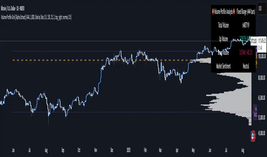
Volume Profile Grid [Alpha Extract]A sophisticated volume distribution analysis system that transforms market activity into institutional-grade visual profiles, revealing hidden support/resistance zones and market participant behavior. Utilizing advanced price level segmentation, bullish/bearish volume separation, and dynamic range analysis, the Volume Profile Grid delivers comprehensive market structure insights with Point of Control (POC) identification, Value Area boundaries, and volume delta analysis. The system features intelligent visualization modes, real-time sentiment analysis, and flexible range selection to provide traders with clear, actionable volume-based market context.
🔶 Dynamic Range Analysis Engine
Implements dual-mode range selection with visible chart analysis and fixed period lookback, automatically adjusting to current market view or analyzing specified historical periods. The system intelligently calculates optimal bar counts while maintaining performance through configurable maximum limits, ensuring responsive profile generation across all timeframes with institutional-grade precision.
// Dynamic period calculation with intelligent caching
get_analysis_period() =>
if i_use_visible_range
chart_start_time = chart.left_visible_bar_time
current_time = last_bar_time
time_span = current_time - chart_start_time
tf_seconds = timeframe.in_seconds()
estimated_bars = time_span / (tf_seconds * 1000)
range_bars = math.floor(estimated_bars)
final_bars = math.min(range_bars, i_max_visible_bars)
math.max(final_bars, 50) // Minimum threshold
else
math.max(i_periods, 50)
🔶 Advanced Bull/Bear Volume Separation
Employs sophisticated candle classification algorithms to separate bullish and bearish volume at each price level, with weighted distribution based on bar intersection ratios. The system analyzes open/close relationships to determine volume direction, applying proportional allocation for doji patterns and ensuring accurate representation of buying versus selling pressure across the entire price spectrum.
🔶 Multi-Mode Volume Visualization
Features three distinct display modes for bull/bear volume representation: Split mode creates mirrored profiles from a central axis, Side by Side mode displays sequential bull/bear segments, and Stacked mode separates volumes vertically. Each mode offers unique insights into market participant behavior with customizable width, thickness, and color parameters for optimal visual clarity.
// Bull/Bear volume calculation with weighted distribution
for bar_offset = 0 to actual_periods - 1
bar_high = high
bar_low = low
bar_volume = volume
// Calculate intersection weight
weight = math.min(bar_high, next_level) - math.max(bar_low, current_level)
weight := weight / (bar_high - bar_low)
weighted_volume = bar_volume * weight
// Classify volume direction
if bar_close > bar_open
level_bull_volume += weighted_volume
else if bar_close < bar_open
level_bear_volume += weighted_volume
else // Doji handling
level_bull_volume += weighted_volume * 0.5
level_bear_volume += weighted_volume * 0.5
🔶 Point of Control & Value Area Detection
Implements institutional-standard POC identification by locating the price level with maximum volume accumulation, providing critical support/resistance zones. The Value Area calculation uses sophisticated sorting algorithms to identify the price range containing 70% of trading volume, revealing the market's accepted value zone where institutional participants concentrate their activity.
🔶 Volume Delta Analysis System
Incorporates real-time volume delta calculation with configurable dominance thresholds to identify significant bull/bear imbalances. The system visually highlights price levels where buying or selling pressure exceeds threshold percentages, providing immediate insight into directional volume flow and potential reversal zones through color-coded delta indicators.
// Value Area calculation using 70% volume accumulation
total_volume_sum = array.sum(total_volumes)
target_volume = total_volume_sum * 0.70
// Sort volumes to find highest activity zones
for i = 0 to array.size(sorted_volumes) - 2
for j = i + 1 to array.size(sorted_volumes) - 1
if array.get(sorted_volumes, j) > array.get(sorted_volumes, i)
// Swap and track indices for value area boundaries
// Accumulate until 70% threshold reached
for i = 0 to array.size(sorted_indices) - 1
accumulated_volume += vol
array.push(va_levels, array.get(volume_levels, idx))
if accumulated_volume >= target_volume
break
❓How It Works
🔶 Weighted Volume Distribution
Implements proportional volume allocation based on the percentage of each bar that intersects with price levels. When a bar spans multiple levels, volume is distributed proportionally based on the intersection ratio, ensuring precise representation of trading activity across the entire price spectrum without double-counting or volume loss.
🔶 Real-Time Profile Generation
Profiles regenerate on each bar close when in visible range mode, automatically adapting to chart zoom and scroll actions. The system maintains optimal performance through intelligent caching mechanisms and selective line updates, ensuring smooth operation even with maximum resolution settings and extended analysis periods.
🔶 Market Sentiment Analysis
Features comprehensive volume analysis table displaying total volume metrics, bullish/bearish percentages, and overall market sentiment classification. The system calculates volume dominance ratios in real-time, providing immediate insight into whether buyers or sellers control the current price structure with percentage-based sentiment thresholds.
🔶 Visual Profile Mapping
Provides multi-layered visual feedback through colored volume bars, POC line highlighting, Value Area boundaries, and optional delta indicators. The system supports profile mirroring for alternative perspectives, line extension for future reference, and customizable label positioning with detailed price information at critical levels.
Why Choose Volume Profile Grid
The Volume Profile Grid represents the evolution of volume analysis tools, combining traditional volume profile concepts with modern visualization techniques and intelligent analysis algorithms. By integrating dynamic range selection, sophisticated bull/bear separation, and multi-mode visualization with POC/Value Area detection, it provides traders with institutional-quality market structure analysis that adapts to any trading style. The comprehensive delta analysis and sentiment monitoring system eliminates guesswork while the flexible visualization options ensure optimal clarity across all market conditions, making it an essential tool for traders seeking to understand true market dynamics through volume-based price discovery.
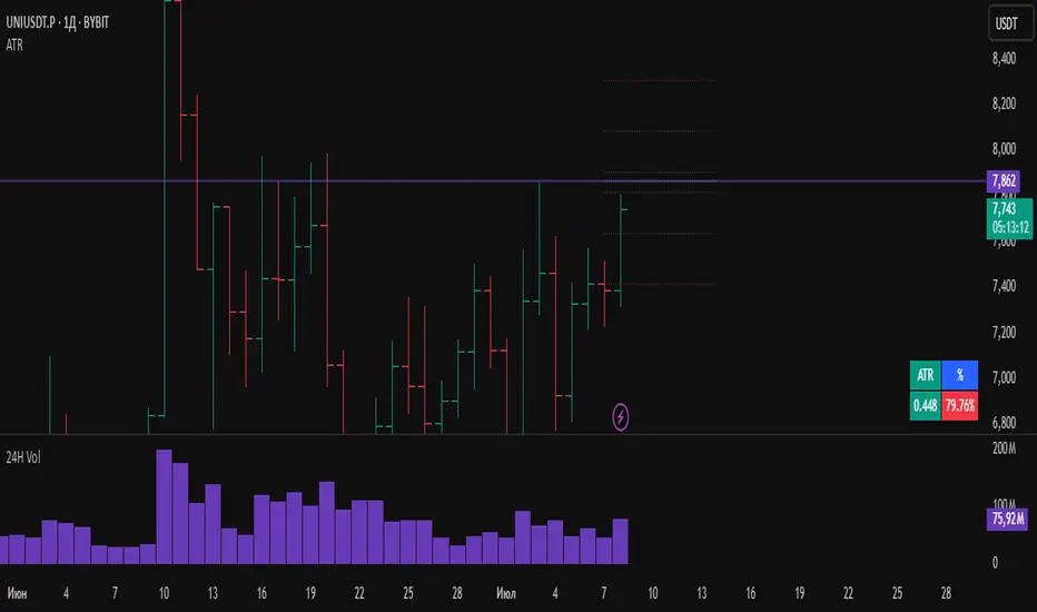
ATRWhat the Indicator Shows:
A compact table with four cells is displayed in the bottom-left corner of the chart:
| ATR | % | Level | Lvl+ATR |
Explanation of the Columns:
ATR — The averaged daily range (volatility) calculated with filtering of abnormal bars (extremely large or small daily candles are ignored).
% — The percentage of the daily ATR that the price has already covered today (the difference between the daily Open and Close relative to ATR).
Level — A custom user-defined level set through the indicator settings.
Lvl+ATR — The sum of the daily ATR and the user-defined level. This can be used, for example, as a target or stop-loss reference.
Color Highlighting of the "%" Cell:
The background color of the "%" ATR cell changes depending on the value:
✅ If the value is less than 10% — the cell is green (market is calm, small movement).
➖ If the value is between 10% and 50% — no highlighting (average movement, no signal).
🟡 If the value is between 50% and 70% — the cell is yellow (movement is increasing, be alert).
🔴 If the value is above 70% — the cell is red (the market is actively moving, high volatility).
Key Features:
✔ All ATR calculations and percentage progress are performed strictly based on daily data, regardless of the chart's current timeframe.
✔ The indicator is ideal for intraday traders who want to monitor daily volatility levels.
✔ The table always displays up-to-date information for quick decision-making.
✔ Filtering of abnormal bars makes ATR more stable and objective.
What is Adaptive ATR in this Indicator:
Instead of the classic ATR, which simply averages the true range, this indicator uses a custom algorithm:
✅ It analyzes daily bars over the past 100 days.
✅ Calculates the range High - Low for each bar.
✅ If the bar's range deviates too much from the average (more than 1.8 times higher or lower), the bar is considered abnormal and ignored.
✅ Only "normal" bars are included in the calculation.
✅ The average range of these normal bars is the adaptive ATR.
Detailed Algorithm of the getAdaptiveATR() Function:
The function takes the number of bars to include in the calculation (for example, 5):
The average of the last 5 normal bars is calculated.
pinescript
Копировать
Редактировать
adaptiveATR = getAdaptiveATR(5)
Step-by-Step Process:
An empty array ranges is created to store the ranges.
Daily bars with indices from 1 to 100 are iterated over.
For each bar:
🔹 The daily High and Low with the required offset are loaded via request.security().
🔹 The range High - Low is calculated.
🔹 The temporary average range of the current array is calculated.
🔹 The bar is checked for abnormality (too large or too small).
🔹 If the bar is normal or it's the first bar — its range is added to the array.
Once the array accumulates the required number of bars (count), their average is calculated — this is the adaptive ATR.
If it's not possible to accumulate the required number of bars — na is returned.
Что показывает индикатор:
На графике внизу слева отображается компактная таблица из четырех ячеек:
ATR % Уровень Ур+ATR
Пояснения к столбцам:
ATR — усреднённый дневной диапазон (волатильность), рассчитанный с фильтрацией аномальных баров (слишком большие или маленькие дневные свечи игнорируются).
% — процент дневного ATR, который уже "прошла" цена на текущий день (разница между открытием и закрытием относительно ATR).
Уровень — пользовательский уровень, который задаётся вручную через настройки индикатора.
Ур+ATR — сумма уровня и дневного ATR. Может использоваться, например, как ориентир для целей или стопов.
Цветовая подсветка ячейки "%":
Цвет фона ячейки с процентом ATR меняется в зависимости от значения:
✅ Если значение меньше 10% — ячейка зелёная (рынок пока спокоен, маленькое движение).
➖ Если значение от 10% до 50% — фон не подсвечивается (среднее движение, нет сигнала).
🟡 Если значение от 50% до 70% — ячейка жёлтая (движение усиливается, повышенное внимание).
🔴 Если значение выше 70% — ячейка красная (рынок активно движется, высокая волатильность).
Особенности работы:
✔ Все расчёты ATR и процентного прохождения производятся исключительно по дневным данным, независимо от текущего таймфрейма графика.
✔ Индикатор подходит для трейдеров, которые торгуют внутри дня, но хотят ориентироваться на дневные уровни волатильности.
✔ В таблице всегда отображается актуальная информация для принятия быстрых торговых решений.
✔ Фильтрация аномальных баров делает ATR более устойчивым и объективным.
Что такое адаптивный ATR в этом индикаторе
Вместо классического ATR, который просто усредняет истинный диапазон, здесь используется собственный алгоритм:
✅ Он берет дневные бары за последние 100 дней.
✅ Для каждого из них рассчитывает диапазон High - Low.
✅ Если диапазон бара слишком сильно отличается от среднего (более чем в 1.8 раза больше или меньше), бар считается аномальным и игнорируется.
✅ Только нормальные бары попадают в расчёт.
✅ В итоге считается среднее из диапазонов этих нормальных баров — это и есть адаптивный ATR.
Подробный алгоритм функции getAdaptiveATR()
Функция принимает количество баров для расчёта (например, 5):
Считается 5 последних нормальных баров
pinescript
Копировать
Редактировать
adaptiveATR = getAdaptiveATR(5)
Пошагово:
Создаётся пустой массив ranges для хранения диапазонов.
Перебираются дневные бары с индексами от 1 до 100.
Для каждого бара:
🔹 Через request.security() подгружаются дневные High и Low с нужным смещением.
🔹 Считается диапазон High - Low.
🔹 Считается временное среднее диапазона по текущему массиву.
🔹 Проверяется, не является ли бар аномальным (слишком большой или маленький).
🔹 Если бар нормальный или это самый первый бар — его диапазон добавляется в массив.
Как только массив набирает заданное количество баров (count), берётся их среднее значение — это и есть адаптивный ATR.
Если не удалось набрать нужное количество баров — возвращается na.
Aetherium Institutional Market Resonance EngineAetherium Institutional Market Resonance Engine (AIMRE)
A Three-Pillar Framework for Decoding Institutional Activity
🎓 THEORETICAL FOUNDATION
The Aetherium Institutional Market Resonance Engine (AIMRE) is a multi-faceted analysis system designed to move beyond conventional indicators and decode the market's underlying structure as dictated by institutional capital flow. Its philosophy is built on a singular premise: significant market moves are preceded by a convergence of context , location , and timing . Aetherium quantifies these three dimensions through a revolutionary three-pillar architecture.
This system is not a simple combination of indicators; it is an integrated engine where each pillar's analysis feeds into a central logic core. A signal is only generated when all three pillars achieve a state of resonance, indicating a high-probability alignment between market organization, key liquidity levels, and cyclical momentum.
⚡ THE THREE-PILLAR ARCHITECTURE
1. 🌌 PILLAR I: THE COHERENCE ENGINE (THE 'CONTEXT')
Purpose: To measure the degree of organization within the market. This pillar answers the question: " Is the market acting with a unified purpose, or is it chaotic and random? "
Conceptual Framework: Institutional campaigns (accumulation or distribution) create a non-random, organized market environment. Retail-driven or directionless markets are characterized by "noise" and chaos. The Coherence Engine acts as a filter to ensure we only engage when institutional players are actively steering the market.
Formulaic Concept:
Coherence = f(Dominance, Synchronization)
Dominance Factor: Calculates the absolute difference between smoothed buying pressure (volume-weighted bullish candles) and smoothed selling pressure (volume-weighted bearish candles), normalized by total pressure. A high value signifies a clear winner between buyers and sellers.
Synchronization Factor: Measures the correlation between the streams of buying and selling pressure over the analysis window. A high positive correlation indicates synchronized, directional activity, while a negative correlation suggests choppy, conflicting action.
The final Coherence score (0-100) represents the percentage of market organization. A high score is a prerequisite for any signal, filtering out unpredictable market conditions.
2. 💎 PILLAR II: HARMONIC LIQUIDITY MATRIX (THE 'LOCATION')
Purpose: To identify and map high-impact institutional footprints. This pillar answers the question: " Where have institutions previously committed significant capital? "
Conceptual Framework: Large institutional orders leave indelible marks on the market in the form of anomalous volume spikes at specific price levels. These are not random occurrences but are areas of intense historical interest. The Harmonic Liquidity Matrix finds these footprints and consolidates them into actionable support and resistance zones called "Harmonic Nodes."
Algorithmic Process:
Footprint Identification: The engine scans the historical lookback period for candles where volume > average_volume * Institutional_Volume_Filter. This identifies statistically significant volume events.
Node Creation: A raw node is created at the mean price of the identified candle.
Dynamic Clustering: The engine uses an ATR-based proximity algorithm. If a new footprint is identified within Node_Clustering_Distance (ATR) of an existing Harmonic Node, it is merged. The node's price is volume-weighted, and its magnitude is increased. This prevents chart clutter and consolidates nearby institutional orders into a single, more significant level.
Node Decay: Nodes that are older than the Institutional_Liquidity_Scanback period are automatically removed from the chart, ensuring the analysis remains relevant to recent market dynamics.
3. 🌊 PILLAR III: CYCLICAL RESONANCE MATRIX (THE 'TIMING')
Purpose: To identify the market's dominant rhythm and its current phase. This pillar answers the question: " Is the market's immediate energy flowing up or down? "
Conceptual Framework: Markets move in waves and cycles of varying lengths. Trading in harmony with the current cyclical phase dramatically increases the probability of success. Aetherium employs a simplified wavelet analysis concept to decompose price action into short, medium, and long-term cycles.
Algorithmic Process:
Cycle Decomposition: The engine calculates three oscillators based on the difference between pairs of Exponential Moving Averages (e.g., EMA8-EMA13 for short cycle, EMA21-EMA34 for medium cycle).
Energy Measurement: The 'energy' of each cycle is determined by its recent volatility (standard deviation). The cycle with the highest energy is designated as the "Dominant Cycle."
Phase Analysis: The engine determines if the dominant cycles are in a bullish phase (rising from a trough) or a bearish phase (falling from a peak).
Cycle Sync: The highest conviction timing signals occur when multiple cycles (e.g., short and medium) are synchronized in the same direction, indicating broad-based momentum.
🔧 COMPREHENSIVE INPUT SYSTEM
Pillar I: Market Coherence Engine
Coherence Analysis Window (10-50, Default: 21): The lookback period for the Coherence Engine.
Lower Values (10-15): Highly responsive to rapid shifts in market control. Ideal for scalping but can be sensitive to noise.
Balanced (20-30): Excellent for day trading, capturing the ebb and flow of institutional sessions.
Higher Values (35-50): Smoother, more stable reading. Best for swing trading and identifying long-term institutional campaigns.
Coherence Activation Level (50-90%, Default: 70%): The minimum market organization required to enable signal generation.
Strict (80-90%): Only allows signals in extremely clear, powerful trends. Fewer, but potentially higher quality signals.
Standard (65-75%): A robust filter that effectively removes choppy conditions while capturing most valid institutional moves.
Lenient (50-60%): Allows signals in less-organized markets. Can be useful in ranging markets but may increase false signals.
Pillar II: Harmonic Liquidity Matrix
Institutional Liquidity Scanback (100-400, Default: 200): How far back the engine looks for institutional footprints.
Short (100-150): Focuses on recent institutional activity, providing highly relevant, immediate levels.
Long (300-400): Identifies major, long-term structural levels. These nodes are often extremely powerful but may be less frequent.
Institutional Volume Filter (1.3-3.0, Default: 1.8): The multiplier for detecting a volume spike.
High (2.5-3.0): Only registers climactic, undeniable institutional volume. Fewer, but more significant nodes.
Low (1.3-1.7): More sensitive, identifying smaller but still relevant institutional interest.
Node Clustering Distance (0.2-0.8 ATR, Default: 0.4): The ATR-based distance for merging nearby nodes.
High (0.6-0.8): Creates wider, more consolidated zones of liquidity.
Low (0.2-0.3): Creates more numerous, precise, and distinct levels.
Pillar III: Cyclical Resonance Matrix
Cycle Resonance Analysis (30-100, Default: 50): The lookback for determining cycle energy and dominance.
Short (30-40): Tunes the engine to faster, shorter-term market rhythms. Best for scalping.
Long (70-100): Aligns the timing component with the larger primary trend. Best for swing trading.
Institutional Signal Architecture
Signal Quality Mode (Professional, Elite, Supreme): Controls the strictness of the three-pillar confluence.
Professional: Loosest setting. May generate signals if two of the three pillars are in strong alignment. Increases signal frequency.
Elite: Balanced setting. Requires a clear, unambiguous resonance of all three pillars. The recommended default.
Supreme: Most stringent. Requires perfect alignment of all three pillars, with each pillar exhibiting exceptionally strong readings (e.g., coherence > 85%). The highest conviction signals.
Signal Spacing Control (5-25, Default: 10): The minimum bars between signals to prevent clutter and redundant alerts.
🎨 ADVANCED VISUAL SYSTEM
The visual architecture of Aetherium is designed not merely for aesthetics, but to provide an intuitive, at-a-glance understanding of the complex data being processed.
Harmonic Liquidity Nodes: The core visual element. Displayed as multi-layered, semi-transparent horizontal boxes.
Magnitude Visualization: The height and opacity of a node's "glow" are proportional to its volume magnitude. More significant nodes appear brighter and larger, instantly drawing the eye to key levels.
Color Coding: Standard nodes are blue/purple, while exceptionally high-magnitude nodes are highlighted in an accent color to denote critical importance.
🌌 Quantum Resonance Field: A dynamic background gradient that visualizes the overall market environment.
Color: Shifts from cool blues/purples (low coherence) to energetic greens/cyans (high coherence and organization), providing instant context.
Intensity: The brightness and opacity of the field are influenced by total market energy (a composite of coherence, momentum, and volume), making powerful market states visually apparent.
💎 Crystalline Lattice Matrix: A geometric web of lines projected from a central moving average.
Mathematical Basis: Levels are projected using multiples of the Golden Ratio (Phi ≈ 1.618) and the ATR. This visualizes the natural harmonic and fractal structure of the market. It is not arbitrary but is based on mathematical principles of market geometry.
🧠 Synaptic Flow Network: A dynamic particle system visualizing the engine's "thought process."
Node Density & Activation: The number of particles and their brightness/color are tied directly to the Market Coherence score. In high-coherence states, the network becomes a dense, bright, and organized web. In chaotic states, it becomes sparse and dim.
⚡ Institutional Energy Waves: Flowing sine waves that visualize market volatility and rhythm.
Amplitude & Speed: The height and speed of the waves are directly influenced by the ATR and volume, providing a feel for market energy.
📊 INSTITUTIONAL CONTROL MATRIX (DASHBOARD)
The dashboard is the central command console, providing a real-time, quantitative summary of each pillar's status.
Header: Displays the script title and version.
Coherence Engine Section:
State: Displays a qualitative assessment of market organization: ◉ PHASE LOCK (High Coherence), ◎ ORGANIZING (Moderate Coherence), or ○ CHAOTIC (Low Coherence). Color-coded for immediate recognition.
Power: Shows the precise Coherence percentage and a directional arrow (↗ or ↘) indicating if organization is increasing or decreasing.
Liquidity Matrix Section:
Nodes: Displays the total number of active Harmonic Liquidity Nodes currently being tracked.
Target: Shows the price level of the nearest significant Harmonic Node to the current price, representing the most immediate institutional level of interest.
Cycle Matrix Section:
Cycle: Identifies the currently dominant market cycle (e.g., "MID ") based on cycle energy.
Sync: Indicates the alignment of the cyclical forces: ▲ BULLISH , ▼ BEARISH , or ◆ DIVERGENT . This is the core timing confirmation.
Signal Status Section:
A unified status bar that provides the final verdict of the engine. It will display "QUANTUM SCAN" during neutral periods, or announce the tier and direction of an active signal (e.g., "◉ TIER 1 BUY ◉" ), highlighted with the appropriate color.
🎯 SIGNAL GENERATION LOGIC
Aetherium's signal logic is built on the principle of strict, non-negotiable confluence.
Condition 1: Context (Coherence Filter): The Market Coherence must be above the Coherence Activation Level. No signals can be generated in a chaotic market.
Condition 2: Location (Liquidity Node Interaction): Price must be actively interacting with a significant Harmonic Liquidity Node.
For a Buy Signal: Price must be rejecting the Node from below (testing it as support).
For a Sell Signal: Price must be rejecting the Node from above (testing it as resistance).
Condition 3: Timing (Cycle Alignment): The Cyclical Resonance Matrix must confirm that the dominant cycles are synchronized with the intended trade direction.
Signal Tiering: The Signal Quality Mode input determines how strictly these three conditions must be met. 'Supreme' mode, for example, might require not only that the conditions are met, but that the Market Coherence is exceptionally high and the interaction with the Node is accompanied by a significant volume spike.
Signal Spacing: A final filter ensures that signals are spaced by a minimum number of bars, preventing over-alerting in a single move.
🚀 ADVANCED TRADING STRATEGIES
The Primary Confluence Strategy: The intended use of the system. Wait for a Tier 1 (Elite/Supreme) or Tier 2 (Professional/Elite) signal to appear on the chart. This represents the alignment of all three pillars. Enter after the signal bar closes, with a stop-loss placed logically on the other side of the Harmonic Node that triggered the signal.
The Coherence Context Strategy: Use the Coherence Engine as a standalone market filter. When Coherence is high (>70%), favor trend-following strategies. When Coherence is low (<50%), avoid new directional trades or favor range-bound strategies. A sharp drop in Coherence during a trend can be an early warning of a trend's exhaustion.
Node-to-Node Trading: In a high-coherence environment, use the Harmonic Liquidity Nodes as both entry points and profit targets. For example, after a BUY signal is generated at one Node, the next Node above it becomes a logical first profit target.
⚖️ RESPONSIBLE USAGE AND LIMITATIONS
Decision Support, Not a Crystal Ball: Aetherium is an advanced decision-support tool. It is designed to identify high-probability conditions based on a model of institutional behavior. It does not predict the future.
Risk Management is Paramount: No indicator can replace a sound risk management plan. Always use appropriate position sizing and stop-losses. The signals provided are probabilistic, not certainties.
Past Performance Disclaimer: The market models used in this script are based on historical data. While robust, there is no guarantee that these patterns will persist in the future. Market conditions can and do change.
Not a "Set and Forget" System: The indicator performs best when its user understands the concepts behind the three pillars. Use the dashboard and visual cues to build a comprehensive view of the market before acting on a signal.
Backtesting is Essential: Before applying this tool to live trading, it is crucial to backtest and forward-test it on your preferred instruments and timeframes to understand its unique behavior and characteristics.
🔮 CONCLUSION
The Aetherium Institutional Market Resonance Engine represents a paradigm shift from single-variable analysis to a holistic, multi-pillar framework. By quantifying the abstract concepts of market context, location, and timing into a unified, logical system, it provides traders with an unprecedented lens into the mechanics of institutional market operations.
It is not merely an indicator, but a complete analytical engine designed to foster a deeper understanding of market dynamics. By focusing on the core principles of institutional order flow, Aetherium empowers traders to filter out market noise, identify key structural levels, and time their entries in harmony with the market's underlying rhythm.
"In all chaos there is a cosmos, in all disorder a secret order." - Carl Jung
— Dskyz, Trade with insight. Trade with confluence. Trade with Aetherium.

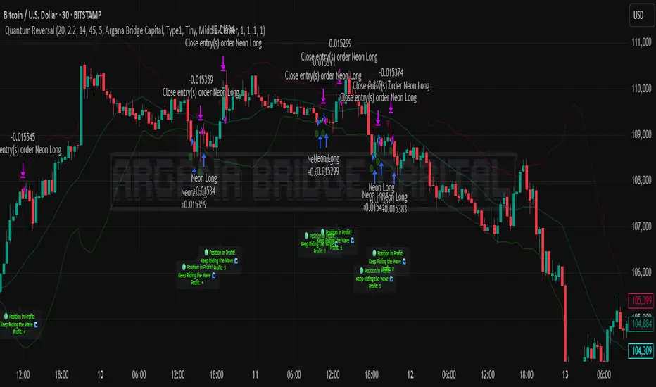
Quantum Reversal# 🧠 Quantum Reversal
## **Quantitative Mean Reversion Framework**
This algorithmic trading system employs **statistical mean reversion theory** combined with **adaptive volatility modeling** to capitalize on Bitcoin's inherent price oscillations around its statistical mean. The strategy integrates multiple technical indicators through a **multi-layered signal processing architecture**.
---
## ⚡ **Core Technical Architecture**
### 📊 **Statistical Foundation**
- **Bollinger Band Mean Reversion Model**: Utilizes 20-period moving average with 2.2 standard deviation bands for volatility-adjusted entry signals
- **Adaptive Volatility Threshold**: Dynamic standard deviation multiplier accounts for Bitcoin's heteroscedastic volatility patterns
- **Price Action Confluence**: Entry triggered when price breaches lower volatility band, indicating statistical oversold conditions
### 🔬 **Momentum Analysis Layer**
- **RSI Oscillator Integration**: 14-period Relative Strength Index with modified oversold threshold at 45
- **Signal Smoothing Algorithm**: 5-period simple moving average applied to RSI reduces noise and false signals
- **Momentum Divergence Detection**: Captures mean reversion opportunities when momentum indicators show oversold readings
### ⚙️ **Entry Logic Architecture**
```
Entry Condition = (Price ≤ Lower_BB) OR (Smoothed_RSI < 45)
```
- **Dual-Condition Framework**: Either statistical price deviation OR momentum oversold condition triggers entry
- **Boolean Logic Gate**: OR-based entry system increases signal frequency while maintaining statistical validity
- **Position Sizing**: Fixed 10% equity allocation per trade for consistent risk exposure
### 🎯 **Exit Strategy Optimization**
- **Profit-Lock Mechanism**: Positions only closed when showing positive unrealized P&L
- **Trend Continuation Logic**: Allows winning trades to run until momentum exhaustion
- **Dynamic Exit Timing**: No fixed profit targets - exits based on profitability state rather than arbitrary levels
---
## 📈 **Statistical Properties**
### **Risk Management Framework**
- **Long-Only Exposure**: Eliminates short-squeeze risk inherent in cryptocurrency markets
- **Mean Reversion Bias**: Exploits Bitcoin's tendency to revert to statistical mean after extreme moves
- **Position Management**: Single position limit prevents over-leveraging
### **Signal Processing Characteristics**
- **Noise Reduction**: SMA smoothing on RSI eliminates high-frequency oscillations
- **Volatility Adaptation**: Bollinger Bands automatically adjust to changing market volatility
- **Multi-Timeframe Coherence**: Indicators operate on consistent timeframe for signal alignment
---
## 🔧 **Parameter Configuration**
| Technical Parameter | Value | Statistical Significance |
|-------------------|-------|-------------------------|
| Bollinger Period | 20 | Standard statistical lookback for volatility calculation |
| Std Dev Multiplier | 2.2 | Optimized for Bitcoin's volatility distribution (95.4% confidence interval) |
| RSI Period | 14 | Traditional momentum oscillator period |
| RSI Threshold | 45 | Modified oversold level accounting for Bitcoin's momentum characteristics |
| Smoothing Period | 5 | Noise reduction filter for momentum signals |
---
## 📊 **Algorithmic Advantages**
✅ **Statistical Edge**: Exploits documented mean reversion tendency in Bitcoin markets
✅ **Volatility Adaptation**: Dynamic bands adjust to changing market conditions
✅ **Signal Confluence**: Multiple indicator confirmation reduces false positives
✅ **Momentum Integration**: RSI smoothing improves signal quality and timing
✅ **Risk-Controlled Exposure**: Systematic position sizing and long-only bias
---
## 🔬 **Mathematical Foundation**
The strategy leverages **Bollinger Band theory** (developed by John Bollinger) which assumes that prices tend to revert to the mean after extreme deviations. The RSI component adds **momentum confirmation** to the statistical price deviation signal.
**Statistical Basis:**
- Mean reversion follows the principle that extreme price deviations from the moving average are temporary
- The 2.2 standard deviation multiplier captures approximately 97.2% of price movements under normal distribution
- RSI momentum smoothing reduces noise inherent in oscillator calculations
---
## ⚠️ **Risk Considerations**
This algorithm is designed for traders with understanding of **quantitative finance principles** and **cryptocurrency market dynamics**. The strategy assumes mean-reverting behavior which may not persist during trending market phases. Proper risk management and position sizing are essential.
---
## 🎯 **Implementation Notes**
- **Market Regime Awareness**: Most effective in ranging/consolidating markets
- **Volatility Sensitivity**: Performance may vary during extreme volatility events
- **Backtesting Recommended**: Historical performance analysis advised before live implementation
- **Capital Allocation**: 10% per trade sizing assumes diversified portfolio approach
---
**Engineered for quantitative traders seeking systematic mean reversion exposure in Bitcoin markets through statistically-grounded technical analysis.**
Tensor Market Analysis Engine (TMAE)# Tensor Market Analysis Engine (TMAE)
## Advanced Multi-Dimensional Mathematical Analysis System
*Where Quantum Mathematics Meets Market Structure*
---
## 🎓 THEORETICAL FOUNDATION
The Tensor Market Analysis Engine represents a revolutionary synthesis of three cutting-edge mathematical frameworks that have never before been combined for comprehensive market analysis. This indicator transcends traditional technical analysis by implementing advanced mathematical concepts from quantum mechanics, information theory, and fractal geometry.
### 🌊 Multi-Dimensional Volatility with Jump Detection
**Hawkes Process Implementation:**
The TMAE employs a sophisticated Hawkes process approximation for detecting self-exciting market jumps. Unlike traditional volatility measures that treat price movements as independent events, the Hawkes process recognizes that market shocks cluster and exhibit memory effects.
**Mathematical Foundation:**
```
Intensity λ(t) = μ + Σ α(t - Tᵢ)
```
Where market jumps at times Tᵢ increase the probability of future jumps through the decay function α, controlled by the Hawkes Decay parameter (0.5-0.99).
**Mahalanobis Distance Calculation:**
The engine calculates volatility jumps using multi-dimensional Mahalanobis distance across up to 5 volatility dimensions:
- **Dimension 1:** Price volatility (standard deviation of returns)
- **Dimension 2:** Volume volatility (normalized volume fluctuations)
- **Dimension 3:** Range volatility (high-low spread variations)
- **Dimension 4:** Correlation volatility (price-volume relationship changes)
- **Dimension 5:** Microstructure volatility (intrabar positioning analysis)
This creates a volatility state vector that captures market behavior impossible to detect with traditional single-dimensional approaches.
### 📐 Hurst Exponent Regime Detection
**Fractal Market Hypothesis Integration:**
The TMAE implements advanced Rescaled Range (R/S) analysis to calculate the Hurst exponent in real-time, providing dynamic regime classification:
- **H > 0.6:** Trending (persistent) markets - momentum strategies optimal
- **H < 0.4:** Mean-reverting (anti-persistent) markets - contrarian strategies optimal
- **H ≈ 0.5:** Random walk markets - breakout strategies preferred
**Adaptive R/S Analysis:**
Unlike static implementations, the TMAE uses adaptive windowing that adjusts to market conditions:
```
H = log(R/S) / log(n)
```
Where R is the range of cumulative deviations and S is the standard deviation over period n.
**Dynamic Regime Classification:**
The system employs hysteresis to prevent regime flipping, requiring sustained Hurst values before regime changes are confirmed. This prevents false signals during transitional periods.
### 🔄 Transfer Entropy Analysis
**Information Flow Quantification:**
Transfer entropy measures the directional flow of information between price and volume, revealing lead-lag relationships that indicate future price movements:
```
TE(X→Y) = Σ p(yₜ₊₁, yₜ, xₜ) log
```
**Causality Detection:**
- **Volume → Price:** Indicates accumulation/distribution phases
- **Price → Volume:** Suggests retail participation or momentum chasing
- **Balanced Flow:** Market equilibrium or transition periods
The system analyzes multiple lag periods (2-20 bars) to capture both immediate and structural information flows.
---
## 🔧 COMPREHENSIVE INPUT SYSTEM
### Core Parameters Group
**Primary Analysis Window (10-100, Default: 50)**
The fundamental lookback period affecting all calculations. Optimization by timeframe:
- **1-5 minute charts:** 20-30 (rapid adaptation to micro-movements)
- **15 minute-1 hour:** 30-50 (balanced responsiveness and stability)
- **4 hour-daily:** 50-100 (smooth signals, reduced noise)
- **Asset-specific:** Cryptocurrency 20-35, Stocks 35-50, Forex 40-60
**Signal Sensitivity (0.1-2.0, Default: 0.7)**
Master control affecting all threshold calculations:
- **Conservative (0.3-0.6):** High-quality signals only, fewer false positives
- **Balanced (0.7-1.0):** Optimal risk-reward ratio for most trading styles
- **Aggressive (1.1-2.0):** Maximum signal frequency, requires careful filtering
**Signal Generation Mode:**
- **Aggressive:** Any component signals (highest frequency)
- **Confluence:** 2+ components agree (balanced approach)
- **Conservative:** All 3 components align (highest quality)
### Volatility Jump Detection Group
**Volatility Dimensions (2-5, Default: 3)**
Determines the mathematical space complexity:
- **2D:** Price + Volume volatility (suitable for clean markets)
- **3D:** + Range volatility (optimal for most conditions)
- **4D:** + Correlation volatility (advanced multi-asset analysis)
- **5D:** + Microstructure volatility (maximum sensitivity)
**Jump Detection Threshold (1.5-4.0σ, Default: 3.0σ)**
Standard deviations required for volatility jump classification:
- **Cryptocurrency:** 2.0-2.5σ (naturally volatile)
- **Stock Indices:** 2.5-3.0σ (moderate volatility)
- **Forex Major Pairs:** 3.0-3.5σ (typically stable)
- **Commodities:** 2.0-3.0σ (varies by commodity)
**Jump Clustering Decay (0.5-0.99, Default: 0.85)**
Hawkes process memory parameter:
- **0.5-0.7:** Fast decay (jumps treated as independent)
- **0.8-0.9:** Moderate clustering (realistic market behavior)
- **0.95-0.99:** Strong clustering (crisis/event-driven markets)
### Hurst Exponent Analysis Group
**Calculation Method Options:**
- **Classic R/S:** Original Rescaled Range (fast, simple)
- **Adaptive R/S:** Dynamic windowing (recommended for trading)
- **DFA:** Detrended Fluctuation Analysis (best for noisy data)
**Trending Threshold (0.55-0.8, Default: 0.60)**
Hurst value defining persistent market behavior:
- **0.55-0.60:** Weak trend persistence
- **0.65-0.70:** Clear trending behavior
- **0.75-0.80:** Strong momentum regimes
**Mean Reversion Threshold (0.2-0.45, Default: 0.40)**
Hurst value defining anti-persistent behavior:
- **0.35-0.45:** Weak mean reversion
- **0.25-0.35:** Clear ranging behavior
- **0.15-0.25:** Strong reversion tendency
### Transfer Entropy Parameters Group
**Information Flow Analysis:**
- **Price-Volume:** Classic flow analysis for accumulation/distribution
- **Price-Volatility:** Risk flow analysis for sentiment shifts
- **Multi-Timeframe:** Cross-timeframe causality detection
**Maximum Lag (2-20, Default: 5)**
Causality detection window:
- **2-5 bars:** Immediate causality (scalping)
- **5-10 bars:** Short-term flow (day trading)
- **10-20 bars:** Structural flow (swing trading)
**Significance Threshold (0.05-0.3, Default: 0.15)**
Minimum entropy for signal generation:
- **0.05-0.10:** Detect subtle information flows
- **0.10-0.20:** Clear causality only
- **0.20-0.30:** Very strong flows only
---
## 🎨 ADVANCED VISUAL SYSTEM
### Tensor Volatility Field Visualization
**Five-Layer Resonance Bands:**
The tensor field creates dynamic support/resistance zones that expand and contract based on mathematical field strength:
- **Core Layer (Purple):** Primary tensor field with highest intensity
- **Layer 2 (Neutral):** Secondary mathematical resonance
- **Layer 3 (Info Blue):** Tertiary harmonic frequencies
- **Layer 4 (Warning Gold):** Outer field boundaries
- **Layer 5 (Success Green):** Maximum field extension
**Field Strength Calculation:**
```
Field Strength = min(3.0, Mahalanobis Distance × Tensor Intensity)
```
The field amplitude adjusts to ATR and mathematical distance, creating dynamic zones that respond to market volatility.
**Radiation Line Network:**
During active tensor states, the system projects directional radiation lines showing field energy distribution:
- **8 Directional Rays:** Complete angular coverage
- **Tapering Segments:** Progressive transparency for natural visual flow
- **Pulse Effects:** Enhanced visualization during volatility jumps
### Dimensional Portal System
**Portal Mathematics:**
Dimensional portals visualize regime transitions using category theory principles:
- **Green Portals (◉):** Trending regime detection (appear below price for support)
- **Red Portals (◎):** Mean-reverting regime (appear above price for resistance)
- **Yellow Portals (○):** Random walk regime (neutral positioning)
**Tensor Trail Effects:**
Each portal generates 8 trailing particles showing mathematical momentum:
- **Large Particles (●):** Strong mathematical signal
- **Medium Particles (◦):** Moderate signal strength
- **Small Particles (·):** Weak signal continuation
- **Micro Particles (˙):** Signal dissipation
### Information Flow Streams
**Particle Stream Visualization:**
Transfer entropy creates flowing particle streams indicating information direction:
- **Upward Streams:** Volume leading price (accumulation phases)
- **Downward Streams:** Price leading volume (distribution phases)
- **Stream Density:** Proportional to information flow strength
**15-Particle Evolution:**
Each stream contains 15 particles with progressive sizing and transparency, creating natural flow visualization that makes information transfer immediately apparent.
### Fractal Matrix Grid System
**Multi-Timeframe Fractal Levels:**
The system calculates and displays fractal highs/lows across five Fibonacci periods:
- **8-Period:** Short-term fractal structure
- **13-Period:** Intermediate-term patterns
- **21-Period:** Primary swing levels
- **34-Period:** Major structural levels
- **55-Period:** Long-term fractal boundaries
**Triple-Layer Visualization:**
Each fractal level uses three-layer rendering:
- **Shadow Layer:** Widest, darkest foundation (width 5)
- **Glow Layer:** Medium white core line (width 3)
- **Tensor Layer:** Dotted mathematical overlay (width 1)
**Intelligent Labeling System:**
Smart spacing prevents label overlap using ATR-based minimum distances. Labels include:
- **Fractal Period:** Time-based identification
- **Topological Class:** Mathematical complexity rating (0, I, II, III)
- **Price Level:** Exact fractal price
- **Mahalanobis Distance:** Current mathematical field strength
- **Hurst Exponent:** Current regime classification
- **Anomaly Indicators:** Visual strength representations (○ ◐ ● ⚡)
### Wick Pressure Analysis
**Rejection Level Mathematics:**
The system analyzes candle wick patterns to project future pressure zones:
- **Upper Wick Analysis:** Identifies selling pressure and resistance zones
- **Lower Wick Analysis:** Identifies buying pressure and support zones
- **Pressure Projection:** Extends lines forward based on mathematical probability
**Multi-Layer Glow Effects:**
Wick pressure lines use progressive transparency (1-8 layers) creating natural glow effects that make pressure zones immediately visible without cluttering the chart.
### Enhanced Regime Background
**Dynamic Intensity Mapping:**
Background colors reflect mathematical regime strength:
- **Deep Transparency (98% alpha):** Subtle regime indication
- **Pulse Intensity:** Based on regime strength calculation
- **Color Coding:** Green (trending), Red (mean-reverting), Neutral (random)
**Smoothing Integration:**
Regime changes incorporate 10-bar smoothing to prevent background flicker while maintaining responsiveness to genuine regime shifts.
### Color Scheme System
**Six Professional Themes:**
- **Dark (Default):** Professional trading environment optimization
- **Light:** High ambient light conditions
- **Classic:** Traditional technical analysis appearance
- **Neon:** High-contrast visibility for active trading
- **Neutral:** Minimal distraction focus
- **Bright:** Maximum visibility for complex setups
Each theme maintains mathematical accuracy while optimizing visual clarity for different trading environments and personal preferences.
---
## 📊 INSTITUTIONAL-GRADE DASHBOARD
### Tensor Field Status Section
**Field Strength Display:**
Real-time Mahalanobis distance calculation with dynamic emoji indicators:
- **⚡ (Lightning):** Extreme field strength (>1.5× threshold)
- **● (Solid Circle):** Strong field activity (>1.0× threshold)
- **○ (Open Circle):** Normal field state
**Signal Quality Rating:**
Democratic algorithm assessment:
- **ELITE:** All 3 components aligned (highest probability)
- **STRONG:** 2 components aligned (good probability)
- **GOOD:** 1 component active (moderate probability)
- **WEAK:** No clear component signals
**Threshold and Anomaly Monitoring:**
- **Threshold Display:** Current mathematical threshold setting
- **Anomaly Level (0-100%):** Combined volatility and volume spike measurement
- **>70%:** High anomaly (red warning)
- **30-70%:** Moderate anomaly (orange caution)
- **<30%:** Normal conditions (green confirmation)
### Tensor State Analysis Section
**Mathematical State Classification:**
- **↑ BULL (Tensor State +1):** Trending regime with bullish bias
- **↓ BEAR (Tensor State -1):** Mean-reverting regime with bearish bias
- **◈ SUPER (Tensor State 0):** Random walk regime (neutral)
**Visual State Gauge:**
Five-circle progression showing tensor field polarity:
- **🟢🟢🟢⚪⚪:** Strong bullish mathematical alignment
- **⚪⚪🟡⚪⚪:** Neutral/transitional state
- **⚪⚪🔴🔴🔴:** Strong bearish mathematical alignment
**Trend Direction and Phase Analysis:**
- **📈 BULL / 📉 BEAR / ➡️ NEUTRAL:** Primary trend classification
- **🌪️ CHAOS:** Extreme information flow (>2.0 flow strength)
- **⚡ ACTIVE:** Strong information flow (1.0-2.0 flow strength)
- **😴 CALM:** Low information flow (<1.0 flow strength)
### Trading Signals Section
**Real-Time Signal Status:**
- **🟢 ACTIVE / ⚪ INACTIVE:** Long signal availability
- **🔴 ACTIVE / ⚪ INACTIVE:** Short signal availability
- **Components (X/3):** Active algorithmic components
- **Mode Display:** Current signal generation mode
**Signal Strength Visualization:**
Color-coded component count:
- **Green:** 3/3 components (maximum confidence)
- **Aqua:** 2/3 components (good confidence)
- **Orange:** 1/3 components (moderate confidence)
- **Gray:** 0/3 components (no signals)
### Performance Metrics Section
**Win Rate Monitoring:**
Estimated win rates based on signal quality with emoji indicators:
- **🔥 (Fire):** ≥60% estimated win rate
- **👍 (Thumbs Up):** 45-59% estimated win rate
- **⚠️ (Warning):** <45% estimated win rate
**Mathematical Metrics:**
- **Hurst Exponent:** Real-time fractal dimension (0.000-1.000)
- **Information Flow:** Volume/price leading indicators
- **📊 VOL:** Volume leading price (accumulation/distribution)
- **💰 PRICE:** Price leading volume (momentum/speculation)
- **➖ NONE:** Balanced information flow
- **Volatility Classification:**
- **🔥 HIGH:** Above 1.5× jump threshold
- **📊 NORM:** Normal volatility range
- **😴 LOW:** Below 0.5× jump threshold
### Market Structure Section (Large Dashboard)
**Regime Classification:**
- **📈 TREND:** Hurst >0.6, momentum strategies optimal
- **🔄 REVERT:** Hurst <0.4, contrarian strategies optimal
- **🎲 RANDOM:** Hurst ≈0.5, breakout strategies preferred
**Mathematical Field Analysis:**
- **Dimensions:** Current volatility space complexity (2D-5D)
- **Hawkes λ (Lambda):** Self-exciting jump intensity (0.00-1.00)
- **Jump Status:** 🚨 JUMP (active) / ✅ NORM (normal)
### Settings Summary Section (Large Dashboard)
**Active Configuration Display:**
- **Sensitivity:** Current master sensitivity setting
- **Lookback:** Primary analysis window
- **Theme:** Active color scheme
- **Method:** Hurst calculation method (Classic R/S, Adaptive R/S, DFA)
**Dashboard Sizing Options:**
- **Small:** Essential metrics only (mobile/small screens)
- **Normal:** Balanced information density (standard desktop)
- **Large:** Maximum detail (multi-monitor setups)
**Position Options:**
- **Top Right:** Standard placement (avoids price action)
- **Top Left:** Wide chart optimization
- **Bottom Right:** Recent price focus (scalping)
- **Bottom Left:** Maximum price visibility (swing trading)
---
## 🎯 SIGNAL GENERATION LOGIC
### Multi-Component Convergence System
**Component Signal Architecture:**
The TMAE generates signals through sophisticated component analysis rather than simple threshold crossing:
**Volatility Component:**
- **Jump Detection:** Mahalanobis distance threshold breach
- **Hawkes Intensity:** Self-exciting process activation (>0.2)
- **Multi-dimensional:** Considers all volatility dimensions simultaneously
**Hurst Regime Component:**
- **Trending Markets:** Price above SMA-20 with positive momentum
- **Mean-Reverting Markets:** Price at Bollinger Band extremes
- **Random Markets:** Bollinger squeeze breakouts with directional confirmation
**Transfer Entropy Component:**
- **Volume Leadership:** Information flow from volume to price
- **Volume Spike:** Volume 110%+ above 20-period average
- **Flow Significance:** Above entropy threshold with directional bias
### Democratic Signal Weighting
**Signal Mode Implementation:**
- **Aggressive Mode:** Any single component triggers signal
- **Confluence Mode:** Minimum 2 components must agree
- **Conservative Mode:** All 3 components must align
**Momentum Confirmation:**
All signals require momentum confirmation:
- **Long Signals:** RSI >50 AND price >EMA-9
- **Short Signals:** RSI <50 AND price 0.6):**
- **Increase Sensitivity:** Catch momentum continuation
- **Lower Mean Reversion Threshold:** Avoid counter-trend signals
- **Emphasize Volume Leadership:** Institutional accumulation/distribution
- **Tensor Field Focus:** Use expansion for trend continuation
- **Signal Mode:** Aggressive or Confluence for trend following
**Range-Bound Markets (Hurst <0.4):**
- **Decrease Sensitivity:** Avoid false breakouts
- **Lower Trending Threshold:** Quick regime recognition
- **Focus on Price Leadership:** Retail sentiment extremes
- **Fractal Grid Emphasis:** Support/resistance trading
- **Signal Mode:** Conservative for high-probability reversals
**Volatile Markets (High Jump Frequency):**
- **Increase Hawkes Decay:** Recognize event clustering
- **Higher Jump Threshold:** Avoid noise signals
- **Maximum Dimensions:** Capture full volatility complexity
- **Reduce Position Sizing:** Risk management adaptation
- **Enhanced Visuals:** Maximum information for rapid decisions
**Low Volatility Markets (Low Jump Frequency):**
- **Decrease Jump Threshold:** Capture subtle movements
- **Lower Hawkes Decay:** Treat moves as independent
- **Reduce Dimensions:** Simplify analysis
- **Increase Position Sizing:** Capitalize on compressed volatility
- **Minimal Visuals:** Reduce distraction in quiet markets
---
## 🚀 ADVANCED TRADING STRATEGIES
### The Mathematical Convergence Method
**Entry Protocol:**
1. **Fractal Grid Approach:** Monitor price approaching significant fractal levels
2. **Tensor Field Confirmation:** Verify field expansion supporting direction
3. **Portal Signal:** Wait for dimensional portal appearance
4. **ELITE/STRONG Quality:** Only trade highest quality mathematical signals
5. **Component Consensus:** Confirm 2+ components agree in Confluence mode
**Example Implementation:**
- Price approaching 21-period fractal high
- Tensor field expanding upward (bullish mathematical alignment)
- Green portal appears below price (trending regime confirmation)
- ELITE quality signal with 3/3 components active
- Enter long position with stop below fractal level
**Risk Management:**
- **Stop Placement:** Below/above fractal level that generated signal
- **Position Sizing:** Based on Mahalanobis distance (higher distance = smaller size)
- **Profit Targets:** Next fractal level or tensor field resistance
### The Regime Transition Strategy
**Regime Change Detection:**
1. **Monitor Hurst Exponent:** Watch for persistent moves above/below thresholds
2. **Portal Color Change:** Regime transitions show different portal colors
3. **Background Intensity:** Increasing regime background intensity
4. **Mathematical Confirmation:** Wait for regime confirmation (hysteresis)
**Trading Implementation:**
- **Trending Transitions:** Trade momentum breakouts, follow trend
- **Mean Reversion Transitions:** Trade range boundaries, fade extremes
- **Random Transitions:** Trade breakouts with tight stops
**Advanced Techniques:**
- **Multi-Timeframe:** Confirm regime on higher timeframe
- **Early Entry:** Enter on regime transition rather than confirmation
- **Regime Strength:** Larger positions during strong regime signals
### The Information Flow Momentum Strategy
**Flow Detection Protocol:**
1. **Monitor Transfer Entropy:** Watch for significant information flow shifts
2. **Volume Leadership:** Strong edge when volume leads price
3. **Flow Acceleration:** Increasing flow strength indicates momentum
4. **Directional Confirmation:** Ensure flow aligns with intended trade direction
**Entry Signals:**
- **Volume → Price Flow:** Enter during accumulation/distribution phases
- **Price → Volume Flow:** Enter on momentum confirmation breaks
- **Flow Reversal:** Counter-trend entries when flow reverses
**Optimization:**
- **Scalping:** Use immediate flow detection (2-5 bar lag)
- **Swing Trading:** Use structural flow (10-20 bar lag)
- **Multi-Asset:** Compare flow between correlated assets
### The Tensor Field Expansion Strategy
**Field Mathematics:**
The tensor field expansion indicates mathematical pressure building in market structure:
**Expansion Phases:**
1. **Compression:** Field contracts, volatility decreases
2. **Tension Building:** Mathematical pressure accumulates
3. **Expansion:** Field expands rapidly with directional movement
4. **Resolution:** Field stabilizes at new equilibrium
**Trading Applications:**
- **Compression Trading:** Prepare for breakout during field contraction
- **Expansion Following:** Trade direction of field expansion
- **Reversion Trading:** Fade extreme field expansion
- **Multi-Dimensional:** Consider all field layers for confirmation
### The Hawkes Process Event Strategy
**Self-Exciting Jump Trading:**
Understanding that market shocks cluster and create follow-on opportunities:
**Jump Sequence Analysis:**
1. **Initial Jump:** First volatility jump detected
2. **Clustering Phase:** Hawkes intensity remains elevated
3. **Follow-On Opportunities:** Additional jumps more likely
4. **Decay Period:** Intensity gradually decreases
**Implementation:**
- **Jump Confirmation:** Wait for mathematical jump confirmation
- **Direction Assessment:** Use other components for direction
- **Clustering Trades:** Trade subsequent moves during high intensity
- **Decay Exit:** Exit positions as Hawkes intensity decays
### The Fractal Confluence System
**Multi-Timeframe Fractal Analysis:**
Combining fractal levels across different periods for high-probability zones:
**Confluence Zones:**
- **Double Confluence:** 2 fractal levels align
- **Triple Confluence:** 3+ fractal levels cluster
- **Mathematical Confirmation:** Tensor field supports the level
- **Information Flow:** Transfer entropy confirms direction
**Trading Protocol:**
1. **Identify Confluence:** Find 2+ fractal levels within 1 ATR
2. **Mathematical Support:** Verify tensor field alignment
3. **Signal Quality:** Wait for STRONG or ELITE signal
4. **Risk Definition:** Use fractal level for stop placement
5. **Profit Targeting:** Next major fractal confluence zone
---
## ⚠️ COMPREHENSIVE RISK MANAGEMENT
### Mathematical Position Sizing
**Mahalanobis Distance Integration:**
Position size should inversely correlate with mathematical field strength:
```
Position Size = Base Size × (Threshold / Mahalanobis Distance)
```
**Risk Scaling Matrix:**
- **Low Field Strength (<2.0):** Standard position sizing
- **Moderate Field Strength (2.0-3.0):** 75% position sizing
- **High Field Strength (3.0-4.0):** 50% position sizing
- **Extreme Field Strength (>4.0):** 25% position sizing or no trade
### Signal Quality Risk Adjustment
**Quality-Based Position Sizing:**
- **ELITE Signals:** 100% of planned position size
- **STRONG Signals:** 75% of planned position size
- **GOOD Signals:** 50% of planned position size
- **WEAK Signals:** No position or paper trading only
**Component Agreement Scaling:**
- **3/3 Components:** Full position size
- **2/3 Components:** 75% position size
- **1/3 Components:** 50% position size or skip trade
### Regime-Adaptive Risk Management
**Trending Market Risk:**
- **Wider Stops:** Allow for trend continuation
- **Trend Following:** Trade with regime direction
- **Higher Position Size:** Trend probability advantage
- **Momentum Stops:** Trail stops based on momentum indicators
**Mean-Reverting Market Risk:**
- **Tighter Stops:** Quick exits on trend continuation
- **Contrarian Positioning:** Trade against extremes
- **Smaller Position Size:** Higher reversal failure rate
- **Level-Based Stops:** Use fractal levels for stops
**Random Market Risk:**
- **Breakout Focus:** Trade only clear breakouts
- **Tight Initial Stops:** Quick exit if breakout fails
- **Reduced Frequency:** Skip marginal setups
- **Range-Based Targets:** Profit targets at range boundaries
### Volatility-Adaptive Risk Controls
**High Volatility Periods:**
- **Reduced Position Size:** Account for wider price swings
- **Wider Stops:** Avoid noise-based exits
- **Lower Frequency:** Skip marginal setups
- **Faster Exits:** Take profits more quickly
**Low Volatility Periods:**
- **Standard Position Size:** Normal risk parameters
- **Tighter Stops:** Take advantage of compressed ranges
- **Higher Frequency:** Trade more setups
- **Extended Targets:** Allow for compressed volatility expansion
### Multi-Timeframe Risk Alignment
**Higher Timeframe Trend:**
- **With Trend:** Standard or increased position size
- **Against Trend:** Reduced position size or skip
- **Neutral Trend:** Standard position size with tight management
**Risk Hierarchy:**
1. **Primary:** Current timeframe signal quality
2. **Secondary:** Higher timeframe trend alignment
3. **Tertiary:** Mathematical field strength
4. **Quaternary:** Market regime classification
---
## 📚 EDUCATIONAL VALUE AND MATHEMATICAL CONCEPTS
### Advanced Mathematical Concepts
**Tensor Analysis in Markets:**
The TMAE introduces traders to tensor analysis, a branch of mathematics typically reserved for physics and advanced engineering. Tensors provide a framework for understanding multi-dimensional market relationships that scalar and vector analysis cannot capture.
**Information Theory Applications:**
Transfer entropy implementation teaches traders about information flow in markets, a concept from information theory that quantifies directional causality between variables. This provides intuition about market microstructure and participant behavior.
**Fractal Geometry in Trading:**
The Hurst exponent calculation exposes traders to fractal geometry concepts, helping understand that markets exhibit self-similar patterns across multiple timeframes. This mathematical insight transforms how traders view market structure.
**Stochastic Process Theory:**
The Hawkes process implementation introduces concepts from stochastic process theory, specifically self-exciting point processes. This provides mathematical framework for understanding why market events cluster and exhibit memory effects.
### Learning Progressive Complexity
**Beginner Mathematical Concepts:**
- **Volatility Dimensions:** Understanding multi-dimensional analysis
- **Regime Classification:** Learning market personality types
- **Signal Democracy:** Algorithmic consensus building
- **Visual Mathematics:** Interpreting mathematical concepts visually
**Intermediate Mathematical Applications:**
- **Mahalanobis Distance:** Statistical distance in multi-dimensional space
- **Rescaled Range Analysis:** Fractal dimension measurement
- **Information Entropy:** Quantifying uncertainty and causality
- **Field Theory:** Understanding mathematical fields in market context
**Advanced Mathematical Integration:**
- **Tensor Field Dynamics:** Multi-dimensional market force analysis
- **Stochastic Self-Excitation:** Event clustering and memory effects
- **Categorical Composition:** Mathematical signal combination theory
- **Topological Market Analysis:** Understanding market shape and connectivity
### Practical Mathematical Intuition
**Developing Market Mathematics Intuition:**
The TMAE serves as a bridge between abstract mathematical concepts and practical trading applications. Traders develop intuitive understanding of:
- **How markets exhibit mathematical structure beneath apparent randomness**
- **Why multi-dimensional analysis reveals patterns invisible to single-variable approaches**
- **How information flows through markets in measurable, predictable ways**
- **Why mathematical models provide probabilistic edges rather than certainties**
---
## 🔬 IMPLEMENTATION AND OPTIMIZATION
### Getting Started Protocol
**Phase 1: Observation (Week 1)**
1. **Apply with defaults:** Use standard settings on your primary trading timeframe
2. **Study visual elements:** Learn to interpret tensor fields, portals, and streams
3. **Monitor dashboard:** Observe how metrics change with market conditions
4. **No trading:** Focus entirely on pattern recognition and understanding
**Phase 2: Pattern Recognition (Week 2-3)**
1. **Identify signal patterns:** Note what market conditions produce different signal qualities
2. **Regime correlation:** Observe how Hurst regimes affect signal performance
3. **Visual confirmation:** Learn to read tensor field expansion and portal signals
4. **Component analysis:** Understand which components drive signals in different markets
**Phase 3: Parameter Optimization (Week 4-5)**
1. **Asset-specific tuning:** Adjust parameters for your specific trading instrument
2. **Timeframe optimization:** Fine-tune for your preferred trading timeframe
3. **Sensitivity adjustment:** Balance signal frequency with quality
4. **Visual customization:** Optimize colors and intensity for your trading environment
**Phase 4: Live Implementation (Week 6+)**
1. **Paper trading:** Test signals with hypothetical trades
2. **Small position sizing:** Begin with minimal risk during learning phase
3. **Performance tracking:** Monitor actual vs. expected signal performance
4. **Continuous optimization:** Refine settings based on real performance data
### Performance Monitoring System
**Signal Quality Tracking:**
- **ELITE Signal Win Rate:** Track highest quality signals separately
- **Component Performance:** Monitor which components provide best signals
- **Regime Performance:** Analyze performance across different market regimes
- **Timeframe Analysis:** Compare performance across different session times
**Mathematical Metric Correlation:**
- **Field Strength vs. Performance:** Higher field strength should correlate with better performance
- **Component Agreement vs. Win Rate:** More component agreement should improve win rates
- **Regime Alignment vs. Success:** Trading with mathematical regime should outperform
### Continuous Optimization Process
**Monthly Review Protocol:**
1. **Performance Analysis:** Review win rates, profit factors, and maximum drawdown
2. **Parameter Assessment:** Evaluate if current settings remain optimal
3. **Market Adaptation:** Adjust for changes in market character or volatility
4. **Component Weighting:** Consider if certain components should receive more/less emphasis
**Quarterly Deep Analysis:**
1. **Mathematical Model Validation:** Verify that mathematical relationships remain valid
2. **Regime Distribution:** Analyze time spent in different market regimes
3. **Signal Evolution:** Track how signal characteristics change over time
4. **Correlation Analysis:** Monitor correlations between different mathematical components
---
## 🌟 UNIQUE INNOVATIONS AND CONTRIBUTIONS
### Revolutionary Mathematical Integration
**First-Ever Implementations:**
1. **Multi-Dimensional Volatility Tensor:** First indicator to implement true tensor analysis for market volatility
2. **Real-Time Hawkes Process:** First trading implementation of self-exciting point processes
3. **Transfer Entropy Trading Signals:** First practical application of information theory for trade generation
4. **Democratic Component Voting:** First algorithmic consensus system for signal generation
5. **Fractal-Projected Signal Quality:** First system to predict signal quality at future price levels
### Advanced Visualization Innovations
**Mathematical Visualization Breakthroughs:**
- **Tensor Field Radiation:** Visual representation of mathematical field energy
- **Dimensional Portal System:** Category theory visualization for regime transitions
- **Information Flow Streams:** Real-time visual display of market information transfer
- **Multi-Layer Fractal Grid:** Intelligent spacing and projection system
- **Regime Intensity Mapping:** Dynamic background showing mathematical regime strength
### Practical Trading Innovations
**Trading System Advances:**
- **Quality-Weighted Signal Generation:** Signals rated by mathematical confidence
- **Regime-Adaptive Strategy Selection:** Automatic strategy optimization based on market personality
- **Anti-Spam Signal Protection:** Mathematical prevention of signal clustering
- **Component Performance Tracking:** Real-time monitoring of algorithmic component success
- **Field-Strength Position Sizing:** Mathematical volatility integration for risk management
---
## ⚖️ RESPONSIBLE USAGE AND LIMITATIONS
### Mathematical Model Limitations
**Understanding Model Boundaries:**
While the TMAE implements sophisticated mathematical concepts, traders must understand fundamental limitations:
- **Markets Are Not Purely Mathematical:** Human psychology, news events, and fundamental factors create unpredictable elements
- **Past Performance Limitations:** Mathematical relationships that worked historically may not persist indefinitely
- **Model Risk:** Complex models can fail during unprecedented market conditions
- **Overfitting Potential:** Highly optimized parameters may not generalize to future market conditions
### Proper Implementation Guidelines
**Risk Management Requirements:**
- **Never Risk More Than 2% Per Trade:** Regardless of signal quality
- **Diversification Mandatory:** Don't rely solely on mathematical signals
- **Position Sizing Discipline:** Use mathematical field strength for sizing, not confidence
- **Stop Loss Non-Negotiable:** Every trade must have predefined risk parameters
**Realistic Expectations:**
- **Mathematical Edge, Not Certainty:** The indicator provides probabilistic advantages, not guaranteed outcomes
- **Learning Curve Required:** Complex mathematical concepts require time to master
- **Market Adaptation Necessary:** Parameters must evolve with changing market conditions
- **Continuous Education Important:** Understanding underlying mathematics improves application
### Ethical Trading Considerations
**Market Impact Awareness:**
- **Information Asymmetry:** Advanced mathematical analysis may provide advantages over other market participants
- **Position Size Responsibility:** Large positions based on mathematical signals can impact market structure
- **Sharing Knowledge:** Consider educational contributions to trading community
- **Fair Market Participation:** Use mathematical advantages responsibly within market framework
### Professional Development Path
**Skill Development Sequence:**
1. **Basic Mathematical Literacy:** Understand fundamental concepts before advanced application
2. **Risk Management Mastery:** Develop disciplined risk control before relying on complex signals
3. **Market Psychology Understanding:** Combine mathematical analysis with behavioral market insights
4. **Continuous Learning:** Stay updated on mathematical finance developments and market evolution
---
## 🔮 CONCLUSION
The Tensor Market Analysis Engine represents a quantum leap forward in technical analysis, successfully bridging the gap between advanced pure mathematics and practical trading applications. By integrating multi-dimensional volatility analysis, fractal market theory, and information flow dynamics, the TMAE reveals market structure invisible to conventional analysis while maintaining visual clarity and practical usability.
### Mathematical Innovation Legacy
This indicator establishes new paradigms in technical analysis:
- **Tensor analysis for market volatility understanding**
- **Stochastic self-excitation for event clustering prediction**
- **Information theory for causality-based trade generation**
- **Democratic algorithmic consensus for signal quality enhancement**
- **Mathematical field visualization for intuitive market understanding**
### Practical Trading Revolution
Beyond mathematical innovation, the TMAE transforms practical trading:
- **Quality-rated signals replace binary buy/sell decisions**
- **Regime-adaptive strategies automatically optimize for market personality**
- **Multi-dimensional risk management integrates mathematical volatility measures**
- **Visual mathematical concepts make complex analysis immediately interpretable**
- **Educational value creates lasting improvement in trading understanding**
### Future-Proof Design
The mathematical foundations ensure lasting relevance:
- **Universal mathematical principles transcend market evolution**
- **Multi-dimensional analysis adapts to new market structures**
- **Regime detection automatically adjusts to changing market personalities**
- **Component democracy allows for future algorithmic additions**
- **Mathematical visualization scales with increasing market complexity**
### Commitment to Excellence
The TMAE represents more than an indicator—it embodies a philosophy of bringing rigorous mathematical analysis to trading while maintaining practical utility and visual elegance. Every component, from the multi-dimensional tensor fields to the democratic signal generation, reflects a commitment to mathematical accuracy, trading practicality, and educational value.
### Trading with Mathematical Precision
In an era where markets grow increasingly complex and computational, the TMAE provides traders with mathematical tools previously available only to institutional quantitative research teams. Yet unlike academic mathematical models, the TMAE translates complex concepts into intuitive visual representations and practical trading signals.
By combining the mathematical rigor of tensor analysis, the statistical power of multi-dimensional volatility modeling, and the information-theoretic insights of transfer entropy, traders gain unprecedented insight into market structure and dynamics.
### Final Perspective
Markets, like nature, exhibit profound mathematical beauty beneath apparent chaos. The Tensor Market Analysis Engine serves as a mathematical lens that reveals this hidden order, transforming how traders perceive and interact with market structure.
Through mathematical precision, visual elegance, and practical utility, the TMAE empowers traders to see beyond the noise and trade with the confidence that comes from understanding the mathematical principles governing market behavior.
Trade with mathematical insight. Trade with the power of tensors. Trade with the TMAE.
*"In mathematics, you don't understand things. You just get used to them." - John von Neumann*
*With the TMAE, mathematical market understanding becomes not just possible, but intuitive.*
— Dskyz, Trade with insight. Trade with anticipation.

Institutional Volume Profile# Institutional Volume Profile (IVP) - Advanced Volume Analysis Indicator
## Overview
The Institutional Volume Profile (IVP) is a sophisticated technical analysis tool that combines traditional volume profile analysis with institutional volume detection algorithms. This indicator helps traders identify key price levels where significant institutional activity has occurred, providing insights into market structure and potential support/resistance zones.
## Key Features
### 🎯 Volume Profile Analysis
- **Point of Control (POC)**: Identifies the price level with the highest volume activity
- **Value Area**: Highlights the price range containing a specified percentage (default 70%) of total volume
- **Multi-Row Distribution**: Displays volume distribution across 10-50 price levels for detailed analysis
- **Customizable Period**: Analyze volume profiles over 10-500 bars
### 🏛️ Institutional Volume Detection
- **Pocket Pivot Volume (PPV)**: Detects bullish institutional buying when up-volume exceeds recent down-volume peaks
- **Pivot Negative Volume (PNV)**: Identifies bearish institutional selling when down-volume exceeds recent up-volume peaks
- **Accumulation Detection**: Spots potential accumulation phases with high volume and narrow price ranges
- **Distribution Analysis**: Identifies distribution patterns with high volume but minimal price movement
### 🎨 Visual Customization Options
- **Multiple Color Schemes**: Heat Map, Institutional, Monochrome, and Rainbow themes
- **Bar Styles**: Solid, Gradient, Outlined, and 3D Effect rendering
- **Volume Intensity Display**: Visual intensity based on volume magnitude
- **Flexible Positioning**: Left or right side profile placement
- **Current Price Highlighting**: Real-time price level indication
### 📊 Advanced Visual Features
- **Volume Labels**: Display volume amounts at key price levels
- **Gradient Effects**: Multi-step gradient rendering for enhanced visibility
- **3D Styling**: Shadow effects for professional appearance
- **Opacity Control**: Adjustable transparency (10-100%)
- **Border Customization**: Configurable border width and styling
## How It Works
### Volume Distribution Algorithm
The indicator analyzes each bar within the specified period and distributes its volume proportionally across the price levels it touches. This creates an accurate representation of where trading activity has been concentrated.
### Institutional Detection Logic
- **PPV Trigger**: Current up-bar volume > highest down-volume in lookback period + above volume MA
- **PNV Trigger**: Current down-bar volume > highest up-volume in lookback period + above volume MA
- **Accumulation**: High volume + narrow range + bullish close
- **Distribution**: Very high volume + minimal price movement
### Value Area Calculation
Starting from the POC, the algorithm expands both upward and downward, adding volume until reaching the specified percentage of total volume (default 70%).
## Configuration Parameters
### Profile Settings
- **Profile Period**: 10-500 bars (default: 50)
- **Number of Rows**: 10-50 levels (default: 24)
- **Profile Width**: 10-100% of screen (default: 30%)
- **Value Area %**: 50-90% (default: 70%)
### Institutional Analysis
- **PPV Lookback Days**: 5-20 periods (default: 10)
- **Volume MA Length**: 10-200 periods (default: 50)
- **Institutional Threshold**: 1.0-2.0x multiplier (default: 1.2)
### Visual Controls
- **Bar Style**: Solid, Gradient, Outlined, 3D Effect
- **Color Scheme**: Heat Map, Institutional, Monochrome, Rainbow
- **Profile Position**: Left or Right side
- **Opacity**: 10-100%
- **Show Labels**: Volume amount display toggle
## Interpretation Guide
### Volume Profile Elements
- **Thick Horizontal Bars**: High volume nodes (strong support/resistance)
- **Thin Horizontal Bars**: Low volume nodes (weak levels)
- **White Line (POC)**: Strongest support/resistance level
- **Blue Highlighted Area**: Value Area (fair value zone)
### Institutional Signals
- **Blue Triangles (PPV)**: Bullish institutional buying detected
- **Orange Triangles (PNV)**: Bearish institutional selling detected
- **Color-Coded Bars**: Different colors indicate institutional activity types
### Color Scheme Meanings
- **Heat Map**: Red (high volume) → Orange → Yellow → Gray (low volume)
- **Institutional**: Blue (PPV), Orange (PNV), Aqua (Accumulation), Yellow (Distribution)
- **Monochrome**: Grayscale intensity based on volume
- **Rainbow**: Color-coded by price level position
## Trading Applications
### Support and Resistance
- POC acts as dynamic support/resistance
- High volume nodes indicate strong price levels
- Low volume areas suggest potential breakout zones
### Institutional Activity
- PPV above Value Area: Strong bullish signal
- PNV below Value Area: Strong bearish signal
- Accumulation patterns: Potential upward breakouts
- Distribution patterns: Potential downward pressure
### Market Structure Analysis
- Value Area defines fair value range
- Profile shape indicates market sentiment
- Volume gaps suggest potential price targets
## Alert Conditions
- PPV Detection at current price level
- PNV Detection at current price level
- PPV above Value Area (strong bullish)
- PNV below Value Area (strong bearish)
## Best Practices
1. Use multiple timeframes for confirmation
2. Combine with price action analysis
3. Pay attention to volume context (above/below average)
4. Monitor institutional signals near key levels
5. Consider overall market conditions
## Technical Notes
- Maximum 500 boxes and 100 labels for optimal performance
- Real-time calculations update on each bar close
- Historical analysis uses complete bar data
- Compatible with all TradingView chart types and timeframes
---
*This indicator is designed for educational and informational purposes. Always combine with other analysis methods and risk management strategies.*

DisplayUtilitiesLibrary "DisplayUtilities"
Display utilities for color management and visual presentation
get_direction_color(direction, up_excessive, up_normal, neutral, down_normal, down_excessive)
Get candle color based on direction and color scheme
Parameters:
direction (int) : Direction value (-2, -1, 0, 1, 2)
up_excessive (color) : Color for +2 direction
up_normal (color) : Color for +1 direction
neutral (color) : Color for 0 direction
down_normal (color) : Color for -1 direction
down_excessive (color) : Color for -2 direction
Returns: Appropriate color for the direction
get_candle_paint_directions(paint_opt, body_dir, bar_dir, breakout_dir, combined_dir)
Get candle directions for different painting algorithms
Parameters:
paint_opt (string) : Painting option algorithm
body_dir (int) : Body direction
bar_dir (int) : Bar direction
breakout_dir (int) : Breakout direction
combined_dir (int) : Combined direction
Returns:
get_bias_paint_directions(paint_bias, unified_dir)
Get paint directions based on bias filter
Parameters:
paint_bias (string) : Paint bias option ("All", "Bull Bias", "Bear Bias")
unified_dir (int) : Unified direction
Returns: Directions for two plotcandle series
get_transparency_levels(sf_filtered, fade_option, fade_opacity)
Calculate transparency levels for strength factor filtering
Parameters:
sf_filtered (bool) : Is strength factor filtered
fade_option (string) : Fade option ("Disabled", "Fade Candle", "Do Not Fade Wick", "Do Not Fade Wick and Border")
fade_opacity (int) : Fade opacity percentage
Returns:
get_strength_factor_filter(filter_option, individual_filters)
Generate strength factor filter conditions
Parameters:
filter_option (string) : Filter option string
individual_filters (map) : Map of individual filter conditions
Returns: Boolean filter result
get_signal_bar_condition(signal_option, individual_filters)
Generate signal bar conditions (inverted filters)
Parameters:
signal_option (string) : Signal bar option string
individual_filters (map) : Map of individual filter conditions
Returns: Boolean signal bar result
get_zscore_signal_condition(z_signal_option, z_filters)
Get Z-score signal bar conditions
Parameters:
z_signal_option (string) : Z-score signal option
z_filters (map) : Map of Z-score filters
Returns: Boolean Z-score signal condition
get_standard_colors()
Create a standard color scheme for directions
Returns: Standard color set
apply_zscore_modification(original_dir, z_filtered)
Modify directions for Z-score excess display
Parameters:
original_dir (int) : Original direction
z_filtered (bool) : Is Z-score filtered (shows excess)
Returns: Modified direction (doubled if excess detected)
get_default_fade_colors()
Get default fade colors for strength factor overlay
Returns: Default colors for TV overlay
should_paint_candles(paint_algo)
Check if paint algorithm should show candles
Parameters:
paint_algo (string) : Paint algorithm option
Returns: True if algorithm should display candles
get_signal_bar_char(signal_type, is_bullish)
Get signal bar character based on signal type
Parameters:
signal_type (string) : Signal type ("strength_factor" or "zscore")
is_bullish (bool) : Direction is bullish
Returns: Character and location for plotchar
get_signal_bar_color(signal_type, is_bullish)
Get signal bar colors
Parameters:
signal_type (string) : Signal type ("strength_factor" or "zscore")
is_bullish (bool) : Direction is bullish
Returns: Signal bar color

Why EMA Isn't What You Think It IsMany new traders adopt the Exponential Moving Average (EMA) believing it's simply a "better Simple Moving Average (SMA)". This common misconception leads to fundamental misunderstandings about how EMA works and when to use it.
EMA and SMA differ at their core. SMA use a window of finite number of data points, giving equal weight to each data point in the calculation period. This makes SMA a Finite Impulse Response (FIR) filter in signal processing terms. Remember that FIR means that "all that we need is the 'period' number of data points" to calculate the filter value. Anything beyond the given period is not relevant to FIR filters – much like how a security camera with 14-day storage automatically overwrites older footage, making last month's activity completely invisible regardless of how important it might have been.
EMA, however, is an Infinite Impulse Response (IIR) filter. It uses ALL historical data, with each past price having a diminishing - but never zero - influence on the calculated value. This creates an EMA response that extends infinitely into the past—not just for the last N periods. IIR filters cannot be precise if we give them only a 'period' number of data to work on - they will be off-target significantly due to lack of context, like trying to understand Game of Thrones by watching only the final season and wondering why everyone's so upset about that dragon lady going full pyromaniac.
If we only consider a number of data points equal to the EMA's period, we are capturing no more than 86.5% of the total weight of the EMA calculation. Relying on he period window alone (the warm-up period) will provide only 1 - (1 / e^2) weights, which is approximately 1−0.1353 = 0.8647 = 86.5%. That's like claiming you've read a book when you've skipped the first few chapters – technically, you got most of it, but you probably miss some crucial early context.
▶️ What is period in EMA used for?
What does a period parameter really mean for EMA? When we select a 15-period EMA, we're not selecting a window of 15 data points as with an SMA. Instead, we are using that number to calculate a decay factor (α) that determines how quickly older data loses influence in EMA result. Every trader knows EMA calculation: α = 1 / (1+period) – or at least every trader claims to know this while secretly checking the formula when they need it.
Thinking in terms of "period" seriously restricts EMA. The α parameter can be - should be! - any value between 0.0 and 1.0, offering infinite tuning possibilities of the indicator. When we limit ourselves to whole-number periods that we use in FIR indicators, we can only access a small subset of possible IIR calculations – it's like having access to the entire RGB color spectrum with 16.7 million possible colors but stubbornly sticking to the 8 basic crayons in a child's first art set because the coloring book only mentioned those by name.
For example:
Period 10 → alpha = 0.1818
Period 11 → alpha = 0.1667
What about wanting an alpha of 0.17, which might yield superior returns in your strategy that uses EMA? No whole-number period can provide this! Direct α parameterization offers more precision, much like how an analog tuner lets you find the perfect radio frequency while digital presets force you to choose only from predetermined stations, potentially missing the clearest signal sitting right between channels.
Sidenote: the choice of α = 1 / (1+period) is just a convention from 1970s, probably started by J. Welles Wilder, who popularized the use of the 14-day EMA. It was designed to create an approximate equivalence between EMA and SMA over the same number of periods, even thought SMA needs a period window (as it is FIR filter) and EMA doesn't. In reality, the decay factor α in EMA should be allowed any valye between 0.0 and 1.0, not just some discrete values derived from an integer-based period! Algorithmic systems should find the best α decay for EMA directly, allowing the system to fine-tune at will and not through conversion of integer period to float α decay – though this might put a few traditionalist traders into early retirement. Well, to prevent that, most traditionalist implementations of EMA only use period and no alpha at all. Heaven forbid we disturb people who print their charts on paper, draw trendlines with rulers, and insist the market "feels different" since computers do algotrading!
▶️ Calculating EMAs Efficiently
The standard textbook formula for EMA is:
EMA = CurrentPrice × alpha + PreviousEMA × (1 - alpha)
But did you know that a more efficient version exists, once you apply a tiny bit of high school algebra:
EMA = alpha × (CurrentPrice - PreviousEMA) + PreviousEMA
The first one requires three operations: 2 multiplications + 1 addition. The second one also requires three ops: 1 multiplication + 1 addition + 1 subtraction.
That's pathetic, you say? Not worth implementing? In most computational models, multiplications cost much more than additions/subtractions – much like how ordering dessert costs more than asking for a water refill at restaurants.
Relative CPU cost of float operations :
Addition/Subtraction: ~1 cycle
Multiplication: ~5 cycles (depending on precision and architecture)
Now you see the difference? 2 * 5 + 1 = 11 against 5 + 1 + 1 = 7. That is ≈ 36.36% efficiency gain just by swapping formulas around! And making your high school math teacher proud enough to finally put your test on the refrigerator.
▶️ The Warmup Problem: how to start the EMA sequence right
How do we calculate the first EMA value when there's no previous EMA available? Let's see some possible options used throughout the history:
Start with zero : EMA(0) = 0. This creates stupidly large distortion until enough bars pass for the horrible effect to diminish – like starting a trading account with zero balance but backdating a year of missed trades, then watching your balance struggle to climb out of a phantom debt for months.
Start with first price : EMA(0) = first price. This is better than starting with zero, but still causes initial distortion that will be extra-bad if the first price is an outlier – like forming your entire opinion of a stock based solely on its IPO day price, then wondering why your model is tanking for weeks afterward.
Use SMA for warmup : This is the tradition from the pencil-and-paper era of technical analysis – when calculators were luxury items and "algorithmic trading" meant your broker had neat handwriting. We first calculate an SMA over the initial period, then kickstart the EMA with this average value. It's widely used due to tradition, not merit, creating a mathematical Frankenstein that uses an FIR filter (SMA) during the initial period before abruptly switching to an IIR filter (EMA). This methodology is so aesthetically offensive (abrupt kink on the transition from SMA to EMA) that charting platforms hide these early values entirely, pretending EMA simply doesn't exist until the warmup period passes – the technical analysis equivalent of sweeping dust under the rug.
Use WMA for warmup : This one was never popular because it is harder to calculate with a pencil - compared to using simple SMA for warmup. Weighted Moving Average provides a much better approximation of a starting value as its linear descending profile is much closer to the EMA's decay profile.
These methods all share one problem: they produce inaccurate initial values that traders often hide or discard, much like how hedge funds conveniently report awesome performance "since strategy inception" only after their disastrous first quarter has been surgically removed from the track record.
▶️ A Better Way to start EMA: Decaying compensation
Think of it this way: An ideal EMA uses an infinite history of prices, but we only have data starting from a specific point. This creates a problem - our EMA starts with an incorrect assumption that all previous prices were all zero, all close, or all average – like trying to write someone's biography but only having information about their life since last Tuesday.
But there is a better way. It requires more than high school math comprehension and is more computationally intensive, but is mathematically correct and numerically stable. This approach involves compensating calculated EMA values for the "phantom data" that would have existed before our first price point.
Here's how phantom data compensation works:
We start our normal EMA calculation:
EMA_today = EMA_yesterday + α × (Price_today - EMA_yesterday)
But we add a correction factor that adjusts for the missing history:
Correction = 1 at the start
Correction = Correction × (1-α) after each calculation
We then apply this correction:
True_EMA = Raw_EMA / (1-Correction)
This correction factor starts at 1 (full compensation effect) and gets exponentially smaller with each new price bar. After enough data points, the correction becomes so small (i.e., below 0.0000000001) that we can stop applying it as it is no longer relevant.
Let's see how this works in practice:
For the first price bar:
Raw_EMA = 0
Correction = 1
True_EMA = Price (since 0 ÷ (1-1) is undefined, we use the first price)
For the second price bar:
Raw_EMA = α × (Price_2 - 0) + 0 = α × Price_2
Correction = 1 × (1-α) = (1-α)
True_EMA = α × Price_2 ÷ (1-(1-α)) = Price_2
For the third price bar:
Raw_EMA updates using the standard formula
Correction = (1-α) × (1-α) = (1-α)²
True_EMA = Raw_EMA ÷ (1-(1-α)²)
With each new price, the correction factor shrinks exponentially. After about -log₁₀(1e-10)/log₁₀(1-α) bars, the correction becomes negligible, and our EMA calculation matches what we would get if we had infinite historical data.
This approach provides accurate EMA values from the very first calculation. There's no need to use SMA for warmup or discard early values before output converges - EMA is mathematically correct from first value, ready to party without the awkward warmup phase.
Here is Pine Script 6 implementation of EMA that can take alpha parameter directly (or period if desired), returns valid values from the start, is resilient to dirty input values, uses decaying compensator instead of SMA, and uses the least amount of computational cycles possible.
// Enhanced EMA function with proper initialization and efficient calculation
ema(series float source, simple int period=0, simple float alpha=0)=>
// Input validation - one of alpha or period must be provided
if alpha<=0 and period<=0
runtime.error("Alpha or period must be provided")
// Calculate alpha from period if alpha not directly specified
float a = alpha > 0 ? alpha : 2.0 / math.max(period, 1)
// Initialize variables for EMA calculation
var float ema = na // Stores raw EMA value
var float result = na // Stores final corrected EMA
var float e = 1.0 // Decay compensation factor
var bool warmup = true // Flag for warmup phase
if not na(source)
if na(ema)
// First value case - initialize EMA to zero
// (we'll correct this immediately with the compensation)
ema := 0
result := source
else
// Standard EMA calculation (optimized formula)
ema := a * (source - ema) + ema
if warmup
// During warmup phase, apply decay compensation
e *= (1-a) // Update decay factor
float c = 1.0 / (1.0 - e) // Calculate correction multiplier
result := c * ema // Apply correction
// Stop warmup phase when correction becomes negligible
if e <= 1e-10
warmup := false
else
// After warmup, EMA operates without correction
result := ema
result // Return the properly compensated EMA value
▶️ CONCLUSION
EMA isn't just a "better SMA"—it is a fundamentally different tool, like how a submarine differs from a sailboat – both float, but the similarities end there. EMA responds to inputs differently, weighs historical data differently, and requires different initialization techniques.
By understanding these differences, traders can make more informed decisions about when and how to use EMA in trading strategies. And as EMA is embedded in so many other complex and compound indicators and strategies, if system uses tainted and inferior EMA calculatiomn, it is doing a disservice to all derivative indicators too – like building a skyscraper on a foundation of Jell-O.
The next time you add an EMA to your chart, remember: you're not just looking at a "faster moving average." You're using an INFINITE IMPULSE RESPONSE filter that carries the echo of all previous price actions, properly weighted to help make better trading decisions.
EMA done right might significantly improve the quality of all signals, strategies, and trades that rely on EMA somewhere deep in its algorithmic bowels – proving once again that math skills are indeed useful after high school, no matter what your guidance counselor told you.
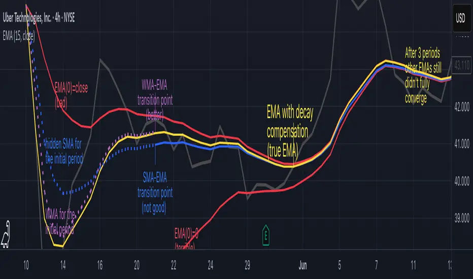
Smarter Money Concepts - OBs [PhenLabs]📊 Smarter Money Concepts - OBs
Version: PineScript™ v6
📌 Description
Smarter Money Concepts - OBs (Order Blocks) is an advanced technical analysis tool designed to identify and visualize institutional order zones on your charts. Order blocks represent significant areas of liquidity where smart money has entered positions before major moves. By tracking these zones, traders can anticipate potential reversals, continuations, and key reaction points in price action.
This indicator incorporates volume filtering technology to identify only the most significant order blocks, eliminating low-quality signals and focusing on areas where institutional participation is likely present. The combination of price structure analysis and volume confirmation provides traders with high-probability zones that may attract future price action for tests, rejections, or breakouts.
🚀 Points of Innovation
Volume-Filtered Block Detection : Identifies only order blocks formed with significant volume, focusing on areas with institutional participation
Advanced Break of Structure Logic : Uses sophisticated price action analysis to detect legitimate market structure breaks preceding order blocks
Dynamic Block Management : Intelligently tracks, extends, and removes order blocks based on price interaction and time-based expiration
Structure Recognition System : Employs technical analysis algorithms to find significant swing points for accurate order block identification
Dual Directional Tracking : Simultaneously monitors both bullish and bearish order blocks for comprehensive market structure analysis
🔧 Core Components
Order Block Detection : Identifies institutional entry zones by analyzing price action before significant breaks of structure, capturing where smart money has likely positioned before moves.
Volume Filtering Algorithm : Calculates relative volume compared to a moving average to qualify only order blocks formed with significant market participation, eliminating noise.
Structure Break Recognition : Uses price action analysis to detect legitimate breaks of market structure, ensuring order blocks are identified only at significant market turning points.
Dynamic Block Management : Continuously monitors price interaction with existing blocks, extending, maintaining, or removing them based on current market behavior.
🔥 Key Features
Volume-Based Filtering : Filter out insignificant blocks by requiring a minimum volume threshold, focusing only on zones with likely institutional activity
Visual Block Highlighting : Color-coded boxes clearly mark bullish and bearish order blocks with customizable appearance
Flexible Mitigation Options : Choose between “Wick” or “Close” methods for determining when a block has been tested or mitigated
Scan Range Adjustment : Customize how far back the indicator looks for structure points to adapt to different market conditions and timeframes
Break Source Selection : Configure which price component (close, open, high, low) is used to determine structure breaks for precise block identification
🎨 Visualization
Bullish Order Blocks : Blue-colored rectangles highlighting zones where bullish institutional orders were likely placed before upward moves, representing potential support areas.
Bearish Order Blocks : Red-colored rectangles highlighting zones where bearish institutional orders were likely placed before downward moves, representing potential resistance areas.
Block Extension : Order blocks extend to the right of the chart, providing clear visualization of these significant zones as price continues to develop.
📖 Usage Guidelines
Order Block Settings
Scan Range : Default: 25. Defines how many bars the indicator scans to determine significant structure points for order block identification.
Bull Break Price Source : Default: Close. Determines which price component is used to detect bullish breaks of structure.
Bear Break Price Source : Default: Close. Determines which price component is used to detect bearish breaks of structure.
Visual Settings
Bullish Blocks Color : Default: Blue with 85% transparency. Controls the appearance of bullish order blocks.
Bearish Blocks Color : Default: Red with 85% transparency. Controls the appearance of bearish order blocks.
General Options
Block Mitigation Method : Default: Wick, Options: Wick, Close. Determines how block mitigation is calculated - “Wick” uses high/low values while “Close” uses close values for more conservative mitigation criteria.
Remove Filled Blocks : Default: Disabled. When enabled, order blocks are removed once they’ve been mitigated by price action.
Volume Filter
Volume Filter Enabled : Default: Enabled. When activated, only shows order blocks formed with significant volume relative to recent average.
Volume SMA Period : Default: 15, Range: 1-50. Number of periods used to calculate the average volume baseline.
Min. Volume Ratio : Default: 1.5, Range: 0.5-10.0. Minimum volume ratio compared to average required to display an order block; higher values filter out more blocks.
✅ Best Use Cases
Identifying high-probability support and resistance zones for trade entries and exits
Finding optimal stop-loss placement behind significant order blocks
Detecting potential reversal areas where price may react after extended moves
Confirming breakout trades when price clears major order blocks
Building a comprehensive market structure map for medium to long-term trading decisions
Pinpointing areas where smart money may have positioned before major market moves
⚠️ Limitations
Most effective on higher timeframes (1H and above) where institutional activity is more clearly defined
Can generate multiple signals in choppy market conditions, requiring additional filtering
Volume filtering relies on accurate volume data, which may be less reliable for some securities
Recent market structure changes may invalidate older order blocks not yet automatically removed
Block identification is based on historical price action and may not predict future behavior with certainty
💡 What Makes This Unique
Volume Intelligence : Unlike basic order block indicators, this script incorporates volume analysis to identify only the most significant institutional zones, focusing on quality over quantity.
Structural Precision : Uses sophisticated break of structure algorithms to identify true market turning points, going beyond simple price pattern recognition.
Dynamic Block Management : Implements automatic block tracking, extension, and cleanup to maintain a clean and relevant chart display without manual intervention.
Institutional Focus : Designed specifically to highlight areas where smart money has likely positioned, helping retail traders align with institutional perspectives rather than retail noise.
🔬 How It Works
1. Structure Identification Process :
The indicator continuously scans price action to identify significant swing points and structure levels within the specified range, establishing a foundation for order block recognition.
2. Break Detection :
When price breaks an established structure level (crossing below a significant low for bearish breaks or above a significant high for bullish breaks), the indicator marks this as a potential zone for order block formation.
3. Volume Qualification :
For each potential order block, the algorithm calculates the relative volume compared to the configured period average. Only blocks formed with volume exceeding the minimum ratio threshold are displayed.
4. Block Creation and Management :
Valid order blocks are created, tracked, and managed as price continues to develop. Blocks extend to the right of the chart until they are either mitigated by price action or expire after the designated timeframe.
5. Continuous Monitoring :
The indicator constantly evaluates price interaction with existing blocks, determining when blocks have been tested, mitigated, or invalidated, and updates the visual representation accordingly.
💡 Note:
Order Blocks represent areas where institutional traders have likely established positions and may defend these zones during future price visits. For optimal results, use this indicator in conjunction with other confluent factors such as key support/resistance levels, trendlines, or additional confirmation indicators. The most reliable signals typically occur on higher timeframes where institutional activity is most prominent. Start with the default settings and adjust parameters gradually to match your specific trading instrument and style.
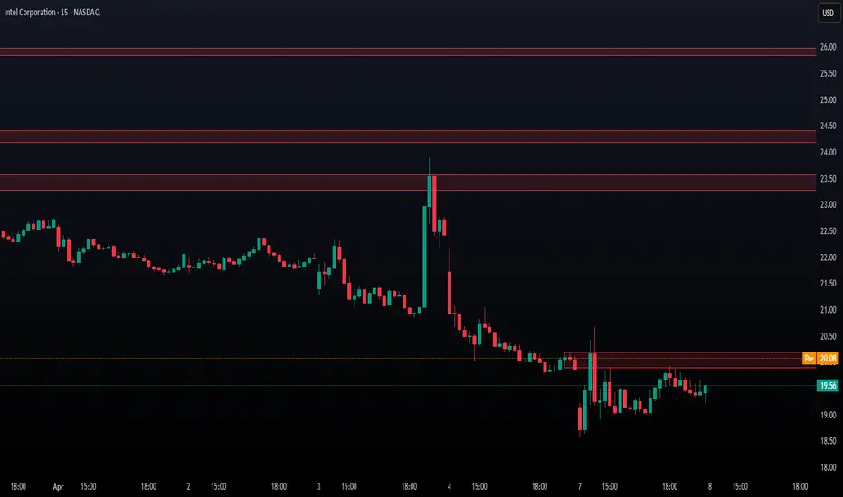
Adaptive Kalman Trend Filter (Zeiierman)█ Overview
The Adaptive Kalman Trend Filter indicator is an advanced trend-following tool designed to help traders accurately identify market trends. Utilizing the Kalman Filter—a statistical algorithm rooted in control theory and signal processing—this indicator adapts to changing market conditions, smoothing price data to filter out noise. By focusing on state vector-based calculations, it dynamically adjusts trend and range measurements, making it an excellent tool for both trend-following and range-based trading strategies. The indicator's adaptive nature is enhanced by options for volatility adjustment and three unique Kalman filter models, each tailored for different market conditions.
█ How It Works
The Kalman Filter works by maintaining a model of the market state through matrices that represent state variables, error covariances, and measurement uncertainties. Here’s how each component plays a role in calculating the indicator’s trend:
⚪ State Vector (X): The state vector is a two-dimensional array where each element represents a market property. The first element is an estimate of the true price, while the second element represents the rate of change or trend in that price. This vector is updated iteratively with each new price, maintaining an ongoing estimate of both price and trend direction.
⚪ Covariance Matrix (P): The covariance matrix represents the uncertainty in the state vector’s estimates. It continuously adapts to changing conditions, representing how much error we expect in our trend and price estimates. Lower covariance values suggest higher confidence in the estimates, while higher values indicate less certainty, often due to market volatility.
⚪ Process Noise (Q): The process noise matrix (Q) is used to account for uncertainties in price movements that aren’t explained by historical trends. By allowing some degree of randomness, it enables the Kalman Filter to remain responsive to new data without overreacting to minor fluctuations. This noise is particularly useful in smoothing out price movements in highly volatile markets.
⚪ Measurement Noise (R): Measurement noise is an external input representing the reliability of each new price observation. In this indicator, it is represented by the setting Measurement Noise and determines how much weight is given to each new price point. Higher measurement noise makes the indicator less reactive to recent prices, smoothing the trend further.
⚪ Update Equations:
Prediction: The state vector and covariance matrix are first projected forward using a state transition matrix (F), which includes market estimates based on past data. This gives a “predicted” state before the next actual price is known.
Kalman Gain Calculation: The Kalman gain is calculated by comparing the predicted state with the actual price, balancing between the covariance matrix and measurement noise. This gain determines how much of the observed price should influence the state vector.
Correction: The observed price is then compared to the predicted price, and the state vector is updated using this Kalman gain. The updated covariance matrix reflects any adjustment in uncertainty based on the latest data.
█ Three Kalman Filter Models
Standard Model: Assumes that market fluctuations follow a linear progression without external adjustments. It is best suited for stable markets.
Volume Adjusted Model: Adjusts the filter sensitivity based on trading volume. High-volume periods result in stronger trends, making this model suitable for volume-driven assets.
Parkinson Adjusted Model: Uses the Parkinson estimator, accounting for volatility through high-low price ranges, making it effective in markets with high intraday fluctuations.
These models enable traders to choose a filter that aligns with current market conditions, enhancing trend accuracy and responsiveness.
█ Trend Strength
The Trend Strength provides a visual representation of the current trend's strength as a percentage based on oscillator calculations from the Kalman filter. This table divides trend strength into color-coded segments, helping traders quickly assess whether the market is strongly trending or nearing a reversal point. A high trend strength percentage indicates a robust trend, while a low percentage suggests weakening momentum or consolidation.
█ Trend Range
The Trend Range section evaluates the market's directional movement over a specified lookback period, highlighting areas where price oscillations indicate a trend. This calculation assesses how prices vary within the range, offering an indication of trend stability or the likelihood of reversals. By adjusting the trend range setting, traders can fine-tune the indicator’s sensitivity to longer or shorter trends.
█ Sigma Bands
The Sigma Bands in the indicator are based on statistical standard deviations (sigma levels), which act as dynamic support and resistance zones. These bands are calculated using the Kalman Filter's trend estimates and adjusted for volatility (if enabled). The bands expand and contract according to market volatility, providing a unique visualization of price boundaries. In high-volatility periods, the bands widen, offering better protection against false breakouts. During low volatility, the bands narrow, closely tracking price movements. Traders can use these sigma bands to spot potential entry and exit points, aiming for reversion trades or trend continuation setups.
Trend Based
Volatility Based
█ How to Use
Trend Following:
When the Kalman Filter is green, it signals a bullish trend, and when it’s red, it indicates a bearish trend. The Sigma Cloud provides additional insights into trend strength. In a strong bullish trend, the cloud remains below the Kalman Filter line, while in a strong bearish trend, the cloud stays above it. Expansion and contraction of the Sigma Cloud indicate market momentum changes. Rapid expansion suggests an impulsive move, which could either signal the continuation of the trend or be an early sign of a possible trend reversal.
Mean Reversion: Watch for prices touching the upper or lower sigma bands, which often act as dynamic support and resistance.
Volatility Breakouts: Enable volatility-adjusted sigma bands. During high volatility, watch for price movements that extend beyond the bands as potential breakout signals.
Trend Continuation: When the Kalman Filter line aligns with a high trend strength, it signals a continuation in that direction.
█ Settings
Measurement Noise: Adjusts how sensitive the indicator is to price changes. Higher values smooth out fluctuations but delay reaction, while lower values increase sensitivity to short-term changes.
Kalman Filter Model: Choose between the standard, volume-adjusted, and Parkinson-adjusted models based on market conditions.
Band Sigma: Sets the standard deviation used for calculating the sigma bands, directly affecting the width of the dynamic support and resistance.
Volatility Adjusted Bands: Enables bands to dynamically adapt to volatility, increasing their effectiveness in fluctuating markets.
Trend Strength: Defines the lookback period for trend strength calculation. Shorter periods result in more responsive trend strength readings, while longer periods smooth out the calculation.
Trend Range: Specifies the lookback period for the trend range, affecting the assessment of trend stability over time.
-----------------
Disclaimer
The information contained in my Scripts/Indicators/Ideas/Algos/Systems does not constitute financial advice or a solicitation to buy or sell any securities of any type. I will not accept liability for any loss or damage, including without limitation any loss of profit, which may arise directly or indirectly from the use of or reliance on such information.
All investments involve risk, and the past performance of a security, industry, sector, market, financial product, trading strategy, backtest, or individual's trading does not guarantee future results or returns. Investors are fully responsible for any investment decisions they make. Such decisions should be based solely on an evaluation of their financial circumstances, investment objectives, risk tolerance, and liquidity needs.
My Scripts/Indicators/Ideas/Algos/Systems are only for educational purposes!
RSI (Kernel Optimized) | Flux Charts💎 GENERAL OVERVIEW
Introducing our new KDE Optimized RSI Indicator! This indicator adds a new aspect to the well-known RSI indicator, with the help of the KDE (Kernel Density Estimation) algorithm, estimates the probability of a candlestick will be a pivot or not. For more information about the process, please check the "HOW DOES IT WORK ?" section.
Features of the new KDE Optimized RSI Indicator :
A New Approach To Pivot Detection
Customizable KDE Algorithm
Realtime RSI & KDE Dashboard
Alerts For Possible Pivots
Customizable Visuals
❓ HOW TO INTERPRET THE KDE %
The KDE % is a critical metric that reflects how closely the current RSI aligns with the KDE (Kernel Density Estimation) array. In simple terms, it represents the likelihood that the current candlestick is forming a pivot point based on historical data patterns. a low percentage suggests a lower probability of the current candlestick being a pivot point. In these cases, price action is less likely to reverse, and existing trends may continue. At moderate levels, the possibility of a pivot increases, indicating potential trend shifts or consolidations.Traders should start monitoring closely for confirmation signals. An even higher KDE % suggests a strong likelihood that the current candlestick could form a pivot point, which could lead to a reversal or significant price movement. These points often align with overbought or oversold conditions in traditional RSI analysis, making them key moments for potential trade entry or exit.
📌 HOW DOES IT WORK ?
The RSI (Relative Strength Index) is a widely used oscillator among traders. It outputs a value between 0 - 100 and gives a glimpse about the current momentum of the price action. This indicator then calculates the RSI for each candlesticks, and saves them into an array if the candlestick is a pivot. The low & high pivot RSIs' are inserted into two different arrays. Then the a KDE array is calculated for both of the low & high pivot RSI arrays. Explaining the KDE might be too much for this write-up, but for a brief explanation, here are the steps :
1. Define the necessary options for the KDE function. These are : Bandwidth & Nº Steps, Array Range (Array Max - Array Min)
2. After that, create a density range array. The array has (steps * 2 - 1) elements and they are calculated by (arrMin + i * stepCount), i being the index.
3. Then, define a kernel function. This indicator has 3 different kernel distribution modes : Uniform, Gaussian and Sigmoid
4. Then, define a temporary value for the current element of KDE array.
5. For each element E in the pivot RSI array, add "kernel(densityRange.get(i) - E, 1.0 / bandwidth)" to the temporary value.
6. Add 1.0 / arrSize * to the KDE array.
Then the prefix sum array of the KDE array is calculated. For each candlestick, the index closest to it's RSI value in the KDE array is found using binary search. Then for the low pivot KDE calculation, the sum of KDE values from found index to max index is calculated. For the high pivot KDE, the sum of 0 to found index is used. Then if high or low KDE value is greater than the activation threshold determined in the settings, a bearish or bullish arrow is plotted after bar confirmation respectively. The arrows are drawn as long as the KDE value of current candlestick is greater than the threshold. When the KDE value is out of the threshold, a less transparent arrow is drawn, indicating a possible pivot point.
🚩 UNIQUENESS
This indicator combines RSI & KDE Algorithm to get a foresight of possible pivot points. Pivot points are important entry, confirmation and exit points for traders. But to their nature, they can be only detected after more candlesticks are rendered after them. The purpose of this indicator is to alert the traders of possible pivot points using KDE algorithm right away when they are confirmed. The indicator also has a dashboard for realtime view of the current RSI & Bullish or Bearish KDE value. You can fully customize the KDE algorithm and set up alerts for pivot detection.
⚙️ SETTINGS
1. RSI Settings
RSI Length -> The amount of bars taken into account for RSI calculation.
Source -> The source value for RSI calculation.
2. Pivots
Pivot Lengths -> Pivot lengths for both high & low pivots. For example, if this value is set to 21; 21 bars before AND 21 bars after a candlestick must be higher for a candlestick to be a low pivot.
3. KDE
Activation Threshold -> This setting determines the amount of arrows shown. Higher options will result in more arrows being rendered.
Kernel -> The kernel function as explained in the upper section.
Bandwidth -> The bandwidth variable as explained in the upper section. The smoothness of the KDE function is tied to this setting.
Nº Bins -> The Nº Steps variable as explained in the upper section. It determines the precision of the KDE algorithm.
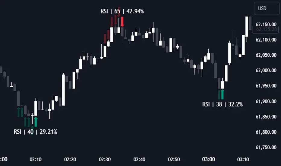
Multiple Naked LevelsPURPOSE OF THE INDICATOR
This indicator autogenerates and displays naked levels and gaps of multiple types collected into one simple and easy to use indicator.
VALUE PROPOSITION OF THE INDICATOR AND HOW IT IS ORIGINAL AND USEFUL
1) CONVENIENCE : The purpose of this indicator is to offer traders with one coherent and robust indicator providing useful, valuable, and often used levels - in one place.
2) CLUSTERS OF CONFLUENCES : With this indicator it is easy to identify levels and zones on the chart with multiple confluences increasing the likelihood of a potential reversal zone.
THE TYPES OF LEVELS AND GAPS INCLUDED IN THE INDICATOR
The types of levels include the following:
1) PIVOT levels (Daily/Weekly/Monthly) depicted in the chart as: dnPIV, wnPIV, mnPIV.
2) POC (Point of Control) levels (Daily/Weekly/Monthly) depicted in the chart as: dnPoC, wnPoC, mnPoC.
3) VAH/VAL STD 1 levels (Value Area High/Low with 1 std) (Daily/Weekly/Monthly) depicted in the chart as: dnVAH1/dnVAL1, wnVAH1/wnVAL1, mnVAH1/mnVAL1
4) VAH/VAL STD 2 levels (Value Area High/Low with 2 std) (Daily/Weekly/Monthly) depicted in the chart as: dnVAH2/dnVAL2, wnVAH2/wnVAL2, mnVAH1/mnVAL2
5) FAIR VALUE GAPS (Daily/Weekly/Monthly) depicted in the chart as: dnFVG, wnFVG, mnFVG.
6) CME GAPS (Daily) depicted in the chart as: dnCME.
7) EQUILIBRIUM levels (Daily/Weekly/Monthly) depicted in the chart as dnEQ, wnEQ, mnEQ.
HOW-TO ACTIVATE LEVEL TYPES AND TIMEFRAMES AND HOW-TO USE THE INDICATOR
You can simply choose which of the levels to be activated and displayed by clicking on the desired radio button in the settings menu.
You can locate the settings menu by clicking into the Object Tree window, left-click on the Multiple Naked Levels and select Settings.
You will then get a menu of different level types and timeframes. Click the checkboxes for the level types and timeframes that you want to display on the chart.
You can then go into the chart and check out which naked levels that have appeared. You can then use those levels as part of your technical analysis.
The levels displayed on the chart can serve as additional confluences or as part of your overall technical analysis and indicators.
In order to back-test the impact of the different naked levels you can also enable tapped levels to be depicted on the chart. Do this by toggling the 'Show tapped levels' checkbox.
Keep in mind however that Trading View can not shom more than 500 lines and text boxes so the indocator will not be able to give you the complete history back to the start for long duration assets.
In order to clean up the charts a little bit there are two additional settings that can be used in the Settings menu:
- Selecting the price range (%) from the current price to be included in the chart. The default is 25%. That means that all levels below or above 20% will not be displayed. You can set this level yourself from 0 up to 100%.
- Selecting the minimum gap size to include on the chart. The default is 1%. That means that all gaps/ranges below 1% in price difference will not be displayed on the chart. You can set the minimum gap size yourself.
BASIC DESCRIPTION OF THE INNER WORKINGS OF THE INDICTATOR
The way the indicator works is that it calculates and identifies all levels from the list of levels type and timeframes above. The indicator then adds this level to a list of untapped levels.
Then for each bar after, it checks if the level has been tapped. If the level has been tapped or a gap/range completely filled, this level is removed from the list so that the levels displayed in the end are only naked/untapped levels.
Below is a descrition of each of the level types and how it is caluclated (algorithm):
PIVOT
Daily, Weekly and Monthly levels in trading refer to significant price points that traders monitor within the context of a single trading day. These levels can provide insights into market behavior and help traders make informed decisions regarding entry and exit points.
Traders often use D/W/M levels to set entry and exit points for trades. For example, entering long positions near support (daily close) or selling near resistance (daily close).
Daily levels are used to set stop-loss orders. Placing stops just below the daily close for long positions or above the daily close for short positions can help manage risk.
The relationship between price movement and daily levels provides insights into market sentiment. For instance, if the price fails to break above the daily high, it may signify bearish sentiment, while a strong breakout can indicate bullish sentiment.
The way these levels are calculated in this indicator is based on finding pivots in the chart on D/W/M timeframe. The level is then set to previous D/W/M close = current D/W/M open.
In addition, when price is going up previous D/W/M open must be smaller than previous D/W/M close and current D/W/M close must be smaller than the current D/W/M open. When price is going down the opposite.
POINT OF CONTROL
The Point of Control (POC) is a key concept in volume profile analysis, which is commonly used in trading.
It represents the price level at which the highest volume of trading occurred during a specific period.
The POC is derived from the volume traded at various price levels over a defined time frame. In this indicator the timeframes are Daily, Weekly, and Montly.
It identifies the price level where the most trades took place, indicating strong interest and activity from traders at that price.
The POC often acts as a significant support or resistance level. If the price approaches the POC from above, it may act as a support level, while if approached from below, it can serve as a resistance level. Traders monitor the POC to gauge potential reversals or breakouts.
The way the POC is calculated in this indicator is by an approximation by analysing intrabars for the respective timeperiod (D/W/M), assigning the volume for each intrabar into the price-bins that the intrabar covers and finally identifying the bin with the highest aggregated volume.
The POC is the price in the middle of this bin.
The indicator uses a sample space for intrabars on the Daily timeframe of 15 minutes, 35 minutes for the Weekly timeframe, and 140 minutes for the Monthly timeframe.
The indicator has predefined the size of the bins to 0.2% of the price at the range low. That implies that the precision of the calulated POC og VAH/VAL is within 0.2%.
This reduction of precision is a tradeoff for performance and speed of the indicator.
This also implies that the bigger the difference from range high prices to range low prices the more bins the algorithm will iterate over. This is typically the case when calculating the monthly volume profile levels and especially high volatility assets such as alt coins.
Sometimes the number of iterations becomes too big for Trading View to handle. In these cases the bin size will be increased even more to reduce the number of iterations.
In such cases the bin size might increase by a factor of 2-3 decreasing the accuracy of the Volume Profile levels.
Anyway, since these Volume Profile levels are approximations and since precision is traded for performance the user should consider the Volume profile levels(POC, VAH, VAL) as zones rather than pin point accurate levels.
VALUE AREA HIGH/LOW STD1/STD2
The Value Area High (VAH) and Value Area Low (VAL) are important concepts in volume profile analysis, helping traders understand price levels where the majority of trading activity occurs for a given period.
The Value Area High/Low is the upper/lower boundary of the value area, representing the highest price level at which a certain percentage of the total trading volume occurred within a specified period.
The VAH/VAL indicates the price point above/below which the majority of trading activity is considered less valuable. It can serve as a potential resistance/support level, as prices above/below this level may experience selling/buying pressure from traders who view the price as overvalued/undervalued
In this indicator the timeframes are Daily, Weekly, and Monthly. This indicator provides two boundaries that can be selected in the menu.
The first boundary is 70% of the total volume (=1 standard deviation from mean). The second boundary is 95% of the total volume (=2 standard deviation from mean).
The way VAH/VAL is calculated is based on the same algorithm as for the POC.
However instead of identifying the bin with the highest volume, we start from range low and sum up the volume for each bin until the aggregated volume = 30%/70% for VAL1/VAH1 and aggregated volume = 5%/95% for VAL2/VAH2.
Then we simply set the VAL/VAH equal to the low of the respective bin.
FAIR VALUE GAPS
Fair Value Gaps (FVG) is a concept primarily used in technical analysis and price action trading, particularly within the context of futures and forex markets. They refer to areas on a price chart where there is a noticeable lack of trading activity, often highlighted by a significant price movement away from a previous level without trading occurring in between.
FVGs represent price levels where the market has moved significantly without any meaningful trading occurring. This can be seen as a "gap" on the price chart, where the price jumps from one level to another, often due to a rapid market reaction to news, events, or other factors.
These gaps typically appear when prices rise or fall quickly, creating a space on the chart where no transactions have taken place. For example, if a stock opens sharply higher and there are no trades at the prices in between the two levels, it creates a gap. The areas within these gaps can be areas of liquidity that the market may return to “fill” later on.
FVGs highlight inefficiencies in pricing and can indicate areas where the market may correct itself. When the market moves rapidly, it may leave behind price levels that traders eventually revisit to establish fair value.
Traders often watch for these gaps as potential reversal or continuation points. Many traders believe that price will eventually “fill” the gap, meaning it will return to those price levels, providing potential entry or exit points.
This indicator calculate FVGs on three different timeframes, Daily, Weekly and Montly.
In this indicator the FVGs are identified by looking for a three-candle pattern on a chart, signalling a discrete imbalance in order volume that prompts a quick price adjustment. These gaps reflect moments where the market sentiment strongly leans towards buying or selling yet lacks the opposite orders to maintain price stability.
The indicator sets the gap to the difference from the high of the first bar to the low of the third bar when price is moving up or from the low of the first bar to the high of the third bar when price is moving down.
CME GAPS (BTC only)
CME gaps refer to price discrepancies that can occur in charts for futures contracts traded on the Chicago Mercantile Exchange (CME). These gaps typically arise from the fact that many futures markets, including those on the CME, operate nearly 24 hours a day but may have significant price movements during periods when the market is closed.
CME gaps occur when there is a difference between the closing price of a futures contract on one trading day and the opening price on the following trading day. This difference can create a "gap" on the price chart.
Opening Gaps: These usually happen when the market opens significantly higher or lower than the previous day's close, often influenced by news, economic data releases, or other market events occurring during non-trading hours.
Gaps can result from reactions to major announcements or developments, such as earnings reports, geopolitical events, or changes in economic indicators, leading to rapid price movements.
The importance of CME Gaps in Trading is the potential for Filling Gaps: Many traders believe that prices often "fill" gaps, meaning that prices may return to the gap area to establish fair value.
This can create potential trading opportunities based on the expectation of gap filling. Gaps can act as significant support or resistance levels. Traders monitor these levels to identify potential reversal points in price action.
The way the gap is identified in this indicator is by checking if current open is higher than previous bar close when price is moving up or if current open is lower than previous day close when price is moving down.
EQUILIBRIUM
Equilibrium in finance and trading refers to a state where supply and demand in a market balance each other, resulting in stable prices. It is a key concept in various economic and trading contexts. Here’s a concise description:
Market Equilibrium occurs when the quantity of a good or service supplied equals the quantity demanded at a specific price level. At this point, there is no inherent pressure for the price to change, as buyers and sellers are in agreement.
Equilibrium Price is the price at which the market is in equilibrium. It reflects the point where the supply curve intersects the demand curve on a graph. At the equilibrium price, the market clears, meaning there are no surplus goods or shortages.
In this indicator the equilibrium level is calculated simply by finding the midpoint of the Daily, Weekly, and Montly candles respectively.
NOTES
1) Performance. The algorithms are quite resource intensive and the time it takes the indicator to calculate all the levels could be 5 seconds or more, depending on the number of bars in the chart and especially if Montly Volume Profile levels are selected (POC, VAH or VAL).
2) Levels displayed vs the selected chart timeframe. On a timeframe smaller than the daily TF - both Daily, Weekly, and Monthly levels will be displayed. On a timeframe bigger than the daily TF but smaller than the weekly TF - the Weekly and Monthly levels will be display but not the Daily levels. On a timeframe bigger than the weekly TF but smaller than the monthly TF - only the Monthly levels will be displayed. Not Daily and Weekly.
CREDITS
The core algorithm for calculating the POC levels is based on the indicator "Naked Intrabar POC" developed by rumpypumpydumpy (https:www.tradingview.com/u/rumpypumpydumpy/).
The "Naked intrabar POC" indicator calculates the POC on the current chart timeframe.
This indicator (Multiple Naked Levels) adds two new features:
1) It calculates the POC on three specific timeframes, the Daily, Weekly, and Monthly timeframes - not only the current chart timeframe.
2) It adds functionaly by calculating the VAL and VAH of the volume profile on the Daily, Weekly, Monthly timeframes .
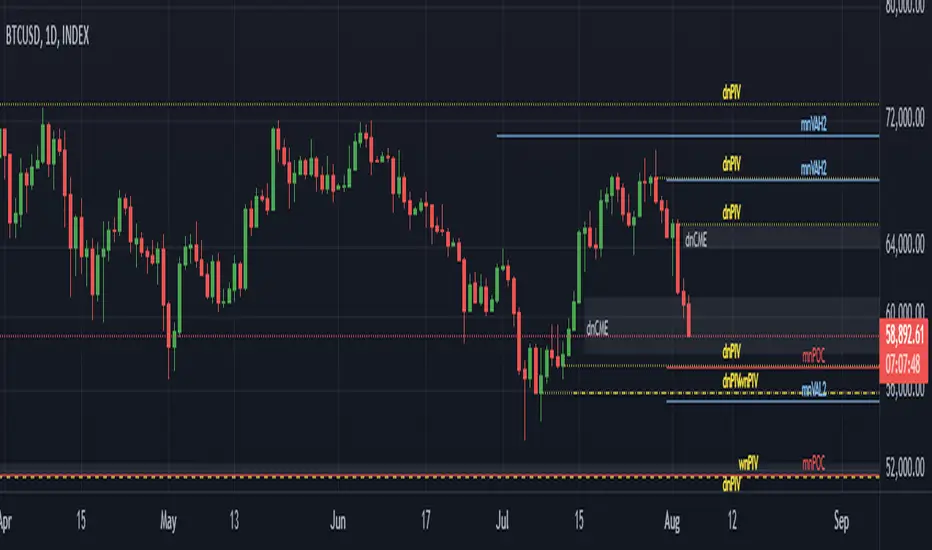
ICT Power Of Three | Flux Charts💎 GENERAL OVERVIEW
Introducing our new ICT Power Of Three Indicator! This indicator is built around the ICT's "Power Of Three" strategy. This strategy makes use of these 3 key smart money concepts : Accumulation, Manipulation and Distribution. Each step is explained in detail within this write-up. For more information about the process, check the "HOW DOES IT WORK" section.
Features of the new ICT Power Of Three Indicator :
Implementation of ICT's Power Of Three Strategy
Different Algorithm Modes
Customizable Execution Settings
Customizable Backtesting Dashboard
Alerts for Buy, Sell, TP & SL Signals
📌 HOW DOES IT WORK ?
The "Power Of Three" comes from these three keywords "Accumulation, Manipulation and Distribution". Here is a brief explanation of each keyword :
Accumulation -> Accumulation phase is when the smart money accumulate their positions in a fixed range. This phase indicates price stability, generally meaning that the price constantly switches between up & down trend between a low and a high pivot point. When the indicator detects an accumulation zone, the Power Of Three strategy begins.
Manipulation -> When the smart money needs to increase their position sizes, they need retail traders' positions for liquidity. So, they manipulate the market into the opposite direction of their intended direction. This will result in retail traders opening positions the way that the smart money intended them to do, creating liquidity. After this step, the real move that the smart money intended begins.
Distribution -> This is when the real intention of the smart money comes into action. With the new liquidity thanks to the manipulation phase, the smart money add their positions towards the opposite direction of the retail mindset. The purpose of this indicator is to detect the accumulation and manipulation phases, and help the trader move towards the same direction as the smart money for their trades.
Detection Methods Of The Indicator :
Accumulation -> The indicator detects accumulation zones as explained step-by-step :
1. Draw two lines from the lowest point and the highest point of the latest X bars.
2. If the (high line - low line) is lower than Average True Range (ATR) * accumulationConstant
3. After the condition is validated, an accumulation zone is detected. The accumulation zone will be invalidated and manipulation phase will begin when the range is broken.
Manipulation -> If the accumulation range is broken, check if the current bar closes / wicks above the (high line + ATR * manipulationConstant) or below the (low line - ATR * manipulationConstant). If the condition is met, the indicator detects a manipulation zone.
Distribution -> The purpose of this indicator is to try to foresee the distribution zone, so instead of a detection, after the manipulation zone is detected the indicator automatically create a "shadow" distribution zone towards the opposite direction of the freshly detected manipulation zone. This shadow distribution zone comes with a take-profit and stop-loss layout, customizable by the trader in the settings.
The X bars, accumulationConstant and manipulationConstant are subject to change with the "Algorithm Mode" setting. Read the "Settings" section for more information.
This indicator follows these steps and inform you step by step by plotting them in your chart.
🚩UNIQUENESS
This indicator is an all-in-one suite for the ICT's Power Of Three concept. It's capable of plotting the strategy, giving signals, a backtesting dashboard and alerts feature. Different and customizable algorithm modes will help the trader fine-tune the indicator for the asset they are currently trading. The backtesting dashboard allows you to see how your settings perform in the current ticker. You can also set up alerts to get informed when the strategy is executable for different tickers.
⚙️SETTINGS
1. General Configuration
Algorithm Mode -> The indicator offers 3 different detection algorithm modes according to your needs. Here is the explanation of each mode.
a) Small Manipulation
This mode has the default bar length for the accumulation detection, but a lower manipulation constant, meaning that slighter imbalances in the price action can be detected as manipulation. This setting can be useful on tickers that have lower liquidity, thus can be manipulated easier.
b) Big Manipulation
This mode has the default bar length for the accumulation detection, but a higher manipulation constant, meaning that heavier imbalances on the price action are required in order to detect manipulation zones. This setting can be useful on tickers that have higher liquidity, thus can be manipulated harder.
c) Short Accumulation
This mode has a ~70% lower bar length requirement for accumulation zone detection, and the default manipulation constant. This setting can be useful on tickers that are highly volatile and do not enter accumulation phases too often.
Breakout Method -> If "Close" is selected, bar close price will be taken into calculation when Accumulation & Manipulation zone invalidation. If "Wick" is selected, a wick will be enough to validate the corresponding zone.
2. TP / SL
TP / SL Method -> If "Fixed" is selected, you can adjust the TP / SL ratios from the settings below. If "Dynamic" is selected, the TP / SL zones will be auto-determined by the algorithm.
Risk -> The risk you're willing to take if "Dynamic" TP / SL Method is selected. Higher risk usually means a better winrate at the cost of losing more if the strategy fails. This setting is has a crucial effect on the performance of the indicator, as different tickers may have different volatility so the indicator may have increased performance when this setting is correctly adjusted.
3. Visuals
Show Zones -> Enables / Disables rendering of Accumulation (yellow) and Manipulation (red) zones.

ICT Concept [TradingFinder] Order Block | FVG | Liquidity Sweeps🔵 Introduction
The "ICT" style is one of the subsets of "Price Action" technical analysis. ICT is a method created by "Michael Huddleston", a professional forex trader and experienced mentor. The acronym ICT stands for "Inner Circle Trader".
The main objective of the ICT trading strategy is to combine "Price Action" and the concept of "Smart Money" to identify optimal entry points into trades. However, finding suitable entry points is not the only strength of this approach. With the ICT style, traders can better understand price behavior and adapt their trading approach to market structure accordingly.
Numerous concepts are discussed in this style, but the key practical concepts for trading in financial markets include "Order Block," "Liquidity," and "FVG".
🔵 How to Use
🟣Order Block
Order blocks are a specific type of "Supply and Demand" zones formed when a series of orders are placed in a block. These orders could be created by banks or other major players. Banks typically execute large orders in blocks during their trading sessions. If they were to enter the market directly with a small quantity, significant price movements would occur before the orders are fully executed, resulting in less profit. To avoid this, they divide their orders into smaller, manageable positions. Traders should look for "buy" opportunities in "demand order blocks" areas and "sell" opportunities in "supply order blocks".
🟣Liquidity
These levels are where traders aim to exit their trades. "Market Makers" or smart money usually collects or distributes their trading positions near levels where many retail traders have placed their "Stop Loss" orders. When the liquidity resulting from these losses is collected, the price often reverses direction.
A "Stop Hunt" is a move designed to neutralize liquidity generated by triggered stop losses. Banks often use significant news events to trigger stop hunts and acquire the liquidity released in the market. If, for example, they intend to execute heavy buy orders, they encourage others to sell through stop hunts.
As a result, if there is liquidity in the market before reaching the order block region, the credibility of that order block is higher. Conversely, if liquidity is near the order block, meaning the price reaches the order block before reaching the liquidity area, the credibility of that order block is lower.
🟣FVG (Fair Value Gap)
To identify the "Fair Value Gap" on the chart, one must analyze candle by candle. Focus on candles with large bodies, examining one candle and the one before it. The candles before and after this central candle should have long shadows, and their bodies should not overlap with the body of the central candle. The distance between the shadows of the first and third candles is called the FVG range.
These zone function in two ways :
•Supply and Demand zone: In this case, the price reacts to these zone, and its trend reverses.
•Liquidity zone: In this scenario, the price "fills" the zone and then reaches the order block.
Important Note: In most cases, FVG zone with very small width act as supply and demand zone, while zone with a significant width act as liquidity zone, absorbing the price.
🔵 Setting
🟣Order Block
Refine Order Block : When the option for refining order blocks is Off, the supply and demand zones encompass the entire length of the order block (from Low to High) in their standard state and remain unaltered. On the option for refining order blocks triggers the improvement of supply and demand zones using the error correction algorithm.
Refine Type : The enhancement of order blocks via the error correction algorithm can be executed through two methods: Defensive and Aggressive. In the Aggressive approach, the widest possible range is taken into account for order blocks.
Show High Levels : If major high levels are to be displayed, set the option for showing high level to Yes.
Show Low Levels : If major low levels are to be displayed, set the option for showing low level to Yes.
Show Last Support : If showing the last support is desired, set the option for showing last support to Yes.
Show Last Resistance : If showing the last resistance is desired, set the option for showing last resistance to Yes.
🟣 FVG
FVG Filter : When FVG filtering is activated, the number of FVG areas undergoes filtration based on the specified algorithm.
FVG Filter Types :
1. Very Aggressive : Apart from the initial condition, an additional condition is introduced. For an upward FVG, the maximum price of the last candle should exceed the maximum price of the middle candle. Similarly, for a downward FVG, the minimum price of the last candle should be lower than the minimum price of the middle candle. This mode eliminates a minimal number of FVGs.
2. Aggressive : In addition to the conditions of the Very Aggressive mode, this mode considers the size of the middle candle; it should not be small. Consequently, a larger number of FVGs are eliminated in this mode.
3. Defensive : Alongside the conditions of the Very Aggressive mode, this mode takes into account the size of the middle candle, which should be relatively large with the majority of it comprising the body. Furthermore, to identify upward FVGs, the second and third candles must be positive, whereas for downward FVGs, the second and third candles must be negative. This mode filters out a considerable number of FVGs, retaining only those of suitable quality.
4. Very Defensive : In addition to the conditions of the Defensive mode, the first and third candles should not be very small-bodied doji candles. This mode filters out the majority of FVGs, leaving only the highest quality ones. Show Demand FVG: Enables the display of demand-related boxes, which can be toggled between off and on. Show Supply FVG: Enables the display of supply-related boxes along the path, which can also be toggled between off and on.
🟣 Liquidity
Statics Liquidity Line Sensitivity : A value ranging from 0 to 0.4. Increasing this value reduces the sensitivity of the "Statics Liquidity Line Detection" function and increases the number of identified lines. The default value is 0.3.
Dynamics Liquidity Line Sensitivity : A value ranging from 0.4 to 1.95. Increasing this value enhances the sensitivity of the "Dynamics Liquidity Line Detection" function and decreases the number of identified lines. The default value is 1.
Statics Period Pivot : Default value is set to 8. By adjusting this value, you can specify the period for static liquidity line pivots.
Dynamics Period Pivot : Default value is set to 3. By adjusting this value, you can specify the period for dynamic liquidity line pivots.
You can activate or deactivate liquidity lines as necessary using the buttons labeled "Show Statics High Liquidity Line," "Show Statics Low Liquidity Line," "Show Dynamics High Liquidity Line," and "Show Dynamics Low Liquidity Line".
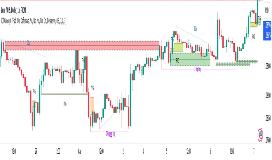
Double AI Super Trend Trading - Strategy [PresentTrading]█ Introduction and How It is Different
The Double AI Super Trend Trading Strategy is a cutting-edge approach that leverages the power of not one, but two AI algorithms, in tandem with the SuperTrend technical indicator. The strategy aims to provide traders with enhanced precision in market entry and exit points. It is designed to adapt to market conditions dynamically, offering the flexibility to trade in both bullish and bearish markets.
*The KNN part is mainly referred from @Zeiierman.
BTCUSD 8hr performance
ETHUSD 8hr performance
█ Strategy, How It Works: Detailed Explanation
1. SuperTrend Calculation
The SuperTrend is a popular indicator that captures market trends through a combination of the Volume-Weighted Moving Average (VWMA) and the Average True Range (ATR). This strategy utilizes two sets of SuperTrend calculations with varying lengths and factors to capture both short-term and long-term market trends.
2. KNN Algorithm
The strategy employs k-Nearest Neighbors (KNN) algorithms, which are supervised machine learning models. Two sets of KNN algorithms are used, each focused on different lengths of historical data and number of neighbors. The KNN algorithms classify the current SuperTrend data point as bullish or bearish based on the weighted sum of the labels of the k closest historical data points.
3. Signal Generation
Based on the KNN classifications and the SuperTrend indicator, the strategy generates signals for the start of a new trend and the continuation of an existing trend.
4. Trading Logic
The strategy uses these signals to enter long or short positions. It also incorporates dynamic trailing stops for exit conditions.
Local picture
█ Trade Direction
The strategy allows traders to specify their trading direction: long, short, or both. This enables the strategy to be versatile and adapt to various market conditions.
█ Usage
ToolTips: Comprehensive tooltips are provided for each parameter to guide the user through the customization process.
Inputs: Traders can customize numerous parameters including the number of neighbors in KNN, ATR multiplier, and types of moving averages.
Plotting: The strategy also provides visual cues on the chart to indicate bullish or bearish trends.
Order Execution: Based on the generated signals, the strategy will execute buy or sell orders automatically.
█ Default Settings
The default settings are configured to offer a balanced approach suitable for most scenarios:
Initial Capital: $10,000
Default Quantity Type: 10% of equity
Commission: 0.1%
Slippage: 1
Currency: USD
These settings can be modified to suit various trading styles and asset classes.
Fibonacci Structure & Trend Channel (Expo)█ Overview
The Fibonacci Structure & Trend Channel (Expo) is designed to identify trend direction and potential reversal levels and offer insights into price structure based on Fibonacci ratios. The algorithm plots a Fibonacci channel, making it easier for traders to identify potential retracement points. Additionally, the Fibonacci market structure is plotted to enhance traders' understanding of the underlying order flow.
█ How to Use
Identify Trends
Use the plotted Fibonacci Trend Line to identify the direction of the market trend. A green line typically signifies a bullish trend, while a red line signifies a bearish trend.
Retracement Levels
The plotted Fibonacci levels can act as potential support or resistance levels. Look for price action signs at these levels for entry or exit points.
Channel Trading
If you enable the Fibonacci channel, the upper and lower bounds can act as overbought or oversold levels.
Market Structure
The plotted Fibonacci market structure serves as a valuable tool for dissecting the underlying order flow and gauging the strength or weakness of a trend. By analyzing these structures, traders can identify key levels where supply and demand intersect, which often act as pivotal points for trend reversals or accelerations. This visual representation simplifies complex market dynamics. Whether you're looking to catch a new trend early or seeking confirmation for a potential reversal, understanding the market structure plotted by the Fibonacci ratios can provide actionable insights for various trading strategies.
Use the Table
The information table can provide quick insights into the current trend and when it started.
█ Settings
The Fibonacci settings allow traders to specify the Fibonacci retracement levels that will be used to calculate the trend and its channel.
The Fibonacci Structure Trend Channel structure settings enable traders to fine-tune how the indicator identifies and plots the underlying price structure.
-----------------
Disclaimer
The information contained in my Scripts/Indicators/Ideas/Algos/Systems does not constitute financial advice or a solicitation to buy or sell any securities of any type. I will not accept liability for any loss or damage, including without limitation any loss of profit, which may arise directly or indirectly from the use of or reliance on such information.
All investments involve risk, and the past performance of a security, industry, sector, market, financial product, trading strategy, backtest, or individual's trading does not guarantee future results or returns. Investors are fully responsible for any investment decisions they make. Such decisions should be based solely on an evaluation of their financial circumstances, investment objectives, risk tolerance, and liquidity needs.
My Scripts/Indicators/Ideas/Algos/Systems are only for educational purposes!
Grid by Volatility (Expo)█ Overview
The Grid by Volatility is designed to provide a dynamic grid overlay on your price chart. This grid is calculated based on the volatility and adjusts in real-time as market conditions change. The indicator uses Standard Deviation to determine volatility and is useful for traders looking to understand price volatility patterns, determine potential support and resistance levels, or validate other trading signals.
█ How It Works
The indicator initiates its computations by assessing the market volatility through an established statistical model: the Standard Deviation. Following the volatility determination, the algorithm calculates a central equilibrium line—commonly referred to as the "mid-line"—on the chart to serve as a baseline for additional computations. Subsequently, upper and lower grid lines are algorithmically generated and plotted equidistantly from the central mid-line, with the distance being dictated by the previously calculated volatility metrics.
█ How to Use
Trend Analysis: The grid can be used to analyze the underlying trend of the asset. For example, if the price is above the Average Line and moves toward the Upper Range, it indicates a strong bullish trend.
Support and Resistance: The grid lines can act as dynamic support and resistance levels. Price tends to bounce off these levels or breakthrough, providing potential trade opportunities.
Volatility Gauge: The distance between the grid lines serves as a measure of market volatility. Wider lines indicate higher volatility, while narrower lines suggest low volatility.
█ Settings
Volatility Length: Number of bars to calculate the Standard Deviation (Default: 200)
Squeeze Adjustment: Multiplier for the Standard Deviation (Default: 6)
Grid Confirmation Length: Number of bars to calculate the weighted moving average for smoothing the grid lines (Default: 2)
-----------------
Disclaimer
The information contained in my Scripts/Indicators/Ideas/Algos/Systems does not constitute financial advice or a solicitation to buy or sell any securities of any type. I will not accept liability for any loss or damage, including without limitation any loss of profit, which may arise directly or indirectly from the use of or reliance on such information.
All investments involve risk, and the past performance of a security, industry, sector, market, financial product, trading strategy, backtest, or individual's trading does not guarantee future results or returns. Investors are fully responsible for any investment decisions they make. Such decisions should be based solely on an evaluation of their financial circumstances, investment objectives, risk tolerance, and liquidity needs.
My Scripts/Indicators/Ideas/Algos/Systems are only for educational purposes!

Filtered Volume Profile [ChartPrime]The "Filtered Volume Profile" is a powerful tool that offers insights into market activity. It's a technical analysis tool used to understand the behavior of financial markets. It uses a fixed range volume profile to provide a histogram representing how much volume occurred at distinct price levels.
Profile in action with various significant levels displayed
How to Use
The script is designed to analyze cumulative trading volumes in different price bins over a certain period, also known as `'lookback'`. This lookback period can be defined by the user and it represents the number of bars to look back for calculating levels of support and resistance.
The `'Smoothing'` input determines the degree to which the output is smoothed. Higher values lead to smoother results but may impede the responsiveness of the indicator to rapid changes in volatility.
The `'Peak Sensitivity'` input is used to adjust the sensitivity of the script's peak detection algorithm. Setting this to a lower value makes the algorithm more sensitive to local changes in trading volume and may result in "noisier" outputs.
The `'Peak Threshold'` input specifies the number of bins that the peak detection mechanism should account for. Larger numbers imply that more volume bins are taken into account, and the resultant peaks are based on wider intervals.
The `'Mean Score Length'` input is used for scaling the mean score range. This is particularly important in defining the length of lookback bars that will be used to calculate the average close price.
Sinc Filter
The application of the sinc-filter to the Filtered Volume Profile reduces the risk of viewing artefacts that may misrepresent the underlying market behavior. Sinc filtering is a high-quality and sharp filter that doesn't manifest any ringing effects, making it an optimal choice for such volume profiling.
Histogram
On the histogram, the volume profile is colored based on the balance of bullish to bearish volume. If a particular bar is more intense in color, it represents a larger than usual volume during a single price bar. This is a clear signal of a strong buying or selling pressure at a particular price level.
Threshold for Peaks
The `peak_thresh` input determines the number of bins the algorithm takes in account for the peak detection feature. The 'peak' represents the level where a significant amount of volume trading has occurred, and usually is of interest as an indicative of support or resistance level.
By increasing the `peak_thresh`, you're raising the bar for what the algorithm perceives as a peak. This could result in fewer, but more significant peaks being identified.
History of Volume Profiles and Evolution into Sinc Filtering
Volume profiling has a rich history in market analysis, dating back to the 1950s when Richard D. Wyckoff, a legendary trader, introduced the concept of volume studies. He understood the critical significance of volume and its relationship with market price movement. The core of Wyckoff's technical analysis suite was the relationship between prices and volume, often termed as "Effort vs Results".
Moving forward, in the early 1800s, the esteemed mathematician J. R. Carson made key improvements to the sinc function, which formed the basis for sinc filtering application in time series data. Following these contributions, trading studies continued to create and integrate more advanced statistical measures into market analysis.
This culminated in the 1980s with J. Peter Steidlmayer’s introduction of Market Profile. He suggested that markets were a function of continuous two-way auction processes thus introducing the concept of viewing markets in price/time continuum and price distribution forms. Steidlmayer's Market Profile was the first wide-scale operation of organized volume and price data.
However, despite the introduction of such features, challenges in the analysis persisted, especially due to noise that could misinform trading decisions. This gap has given rise to the need for smoothing functions to help eliminate the noise and better interpret the data. Among such techniques, the sinc filter has become widely recognized within the trading community.
The sinc filter, because of its properties of constructing a smooth passing through all data points precisely and its ability to eliminate high-frequency noise, has been considered a natural transition in the evolution of volume profile strategies. The superior ability of the sinc filter to reduce noise and shield against over-fitting makes it an ideal choice for smoothing purposes in trading scripts, particularly where volume profiling forms the crux of the market analysis strategy, such as in Filtered Volume Profile.
Moving ahead, the use of volume-based studies seems likely to remain a core part of technical analysis. As long as markets operate based on supply and demand principles, understanding volume will remain key to discerning the intent behind price movements. And with the incorporation of advanced methods like sinc filtering, the accuracy and insight provided by these methodologies will only improve.
Mean Score
The mean score in the Filtered Volume Profile script plays an important role in probabilistic inferences regarding future price direction. This score essentially characterizes the statistical likelihood of price trends based on historical data.
The mean score is calculated over a configurable `'Mean Score Length'`. This variable sets the window or the timeframe for calculation of the mean score of the closing prices.
Statistically, this score takes advantage of the concept of z-scores and probabilities associated with the t-distribution (a type of probability distribution that is symmetric and bell-shaped, just like the standard normal distribution, but has heavier tails).
The z-score represents how many standard deviations an element is from the mean. In this case, the "element" is the price level (Point of Control).
The mean score section of the script calculates standard errors for the root mean squared error (RMSE) and addresses the uncertainty in the prediction of the future value of a random variable.
The RMSE of a model prediction concerning observed values is used to measure the differences between values predicted by a model and the values observed.
The lower the RMSE, the better the model is able to predict. A zero RMSE means a perfect fit to the data. In essence, it's a measure of how concentrated the data is around the line of best fit.
Through the mean score, the script effectively predicts the likelihood of the future close price being above or below our identified price level.
Summary
Filtered Volume Profile is a comprehensive trading view indicator which utilizes volume profiling, peak detection, mean score computations, and sinc-filter smoothing, altogether providing the finer details of market behavior.
It offers a customizable look back period, smoothing options, and peak sensitivity setting along with a uniquely set peak threshold. The application of the Sinc Filter ensures a high level of accuracy and noise reduction in volume profiling, making this script a reliable tool for gaining market insights.
Furthermore, the use of mean score calculations provides probabilistic insights into price movements, thus providing traders with a statistically sound foundation for their trading decisions. As trading markets advance, the use of such methodologies plays a pivotal role in formulating effective trading strategies and the Filtered Volume Profile is a successful embodiment of such advancements in the field of market analysis.
RibboNN Machine Learning [ChartPrime]The RibboNN ML indicator is a powerful tool designed to predict the direction of the market and display it through a ribbon-like visual representation, with colors changing based on the prediction outcome from a conditional class. The primary focus of this indicator is to assist traders in trend following trading strategies.
The RibboNN ML in action
Prediction Process:
Conditional Class: The indicator's predictive model relies on a conditional class, which combines information from both longcon (long condition) and short condition. These conditions are determined using specific rules and criteria, taking into account various market factors and indicators.
Direction Prediction: The conditional class provides the basis for predicting the direction of the market move. When the prediction value is greater than 0, it indicates an upward trend, while a value less than 0 suggests a downward trend.
Nearest Neighbor (NN): To attempt to enhance the accuracy of predictions, the RibboNN ML indicator incorporates a Nearest Neighbor algorithm. This algorithm analyzes historical data from the Ribbon ML's predictive model (RMF) and identifies patterns that closely resemble the current conditional prediction class, thereby offering more robust trend forecasts.
Ribbon Visualization:
The Ribbon ML indicator visually represents its predictions through a ribbon-like display. The ribbon changes colors based on the direction predicted by the conditional class. An upward trend is represented by a green color, while a downward trend is depicted by a red color, allowing traders to quickly identify potential market directions.
The introduction of the Nearest Neighbor algorithm provides the Ribbon ML indicator with unique and adaptive behaviors. By dynamically analyzing historical patterns and incorporating them into predictions, the indicator can adapt to changing market conditions and offer more reliable signals for trend following trading strategies.
Manipulation of the NN Settings:
Smaller Value of Neighbours Count:
When the value of "Neighbours Count" is small, the algorithm considers only a few nearest neighbors for making predictions.
A smaller value of "Neighbours Count" leads to more flexible decision boundaries, which can result in a more granular and sensitive model.
However, using a very small value might lead to overfitting, especially if the training data contains noise or outliers.
Larger Value of "Neighbours Count":
When the value of "Neighbours Count" is large, the algorithm considers a larger number of nearest neighbors for making predictions.
A larger value of "Neighbours Count" leads to smoother decision boundaries and helps capture the global patterns in the data.
However, setting a very large value might result in a loss of local patterns and make the model less sensitive to changes in the data.
Price & Volume Profile (Expo)█ Overview
The Price & Volume Profile provides a holistic perspective on market dynamics by simultaneously tracking price action and trading volume across a range of price levels. So it is not only a volume-based indicator but also a price-based one. In addition to illustrating volume distribution, it quantifies how frequently the price has fallen within a particular range, thus offering a holistic perspective on market dynamics.
This unique and comprehensive approach to market analysis by considering both price action and trading volume, two crucial dimensions of market activity. Its distinctive methodology offers several advantages:
Holistic Market View: By simultaneously tracking the frequency of specific price ranges (Price Profile) and the volume traded at those ranges (Volume Profile), this indicator provides a more complete picture of market behavior. It shows not only where the market is trading but also how much it's trading, reflecting both price acceptance levels and market participation intensity.
Point of Control (POC): The POC, as highlighted by this indicator, serves as a significant reference point for traders. It identifies the price level with the highest trading activity, thus indicating a strong consensus among market participants about the asset's fair value. Observing how price interacts with the POC can offer valuable insights into market sentiment and potential trend reversals.
Support and Resistance Levels: Price levels with high trading activity often act as support or resistance in future price movements. The indicator visually represents these levels, enabling traders to anticipate potential price reactions.
Price Profile
Price and Volume Profile
█ Calculations
The algorithm analyzes both trade frequency and volume across different price levels. It identifies these levels within the visible chart range, then examines each bar to determine if the selected price falls within these levels. If so, it increases a counter and adds the trading volume. This process repeats across the visible range and is visualized as a horizontal histogram, each bar representing a price level and the bar length reflecting trade frequency and volume. Additionally, it calculates the Point of Control (POC), signifying the price level with the highest activity.
In summary: The histogram presents a dual perspective - not only the traded volume at each price level but also the frequency of the price hitting each range. The longer the bar, the more times the price has frequented that specific range, revealing key insights into price behavior and acceptance levels. These frequently visited areas often emerge as strong support or resistance zones, helping traders navigate market movements.
Please note that the indicator adjusts to the visible price range, making it adaptable to changing market conditions. This dynamic analysis can provide more relevant and timely information than static indicators.
█ How to use
This indicator is beneficial for traders as it offers insights into the distribution of trading activity across different price levels. It helps identify key areas of support and resistance and gives a visual representation of market sentiment and liquidity.
The point of control (POC) , which is the price level with the highest traded volume or frequency count, becomes even more crucial in this context. It marks the price at which the most trading activity occurred, signaling a strong consensus among market participants about the asset's fair value. If the market price deviates significantly from the POC, it could suggest an overbought or oversold condition, potentially leading to a price reversion.
Fair Price Areas/gaps are specific price levels or zones where an asset has spent limited time in the past. These areas are considered interesting or significant because they may have an impact on future price action.
Similar to the concept of fair value gaps, which refers to discrepancies between an asset's market price and its estimated intrinsic value, Fair Price Areas/gaps focus on price levels that have been relatively underutilized in terms of trading activity. When an asset's price reaches a Fair Price Area/gap, traders and investors pay attention because they expect the price to react in some way. The rationale behind this concept is that price tends to gravitate towards areas where it has spent less time in the past, as the market perceives them as significant levels.
█ Settings
The indicator is customizable, allowing users to define the number of price levels (rows), the offset, the data source, and whether to display volume or frequency count. It also adjusts dynamically to the visible price range on the chart, ensuring that the analysis remains relevant and timely with changing market conditions.
Source: The price to use for the calculation. Typically, this is the closing price. By considering the user-selected Source (typically the closing price), the indicator determines the frequency with which the price lands within each designated price level (row) over the selected period. In essence, the indicator provides a count of bars where the Source price falls within each range, essentially creating a "Price Profile."
Row Size: The number of price levels (rows) to divide the visible price range into.
Display: Choose whether to display the number of bars ("Counter") or the total volume ("Volume") for each price level.
Offset: The distance of the histogram from the price chart.
Point of Control (POC): If enabled, the indicator will highlight the price level with the most activity.
-----------------
Disclaimer
The information contained in my Scripts/Indicators/Ideas/Algos/Systems does not constitute financial advice or a solicitation to buy or sell any securities of any type. I will not accept liability for any loss or damage, including without limitation any loss of profit, which may arise directly or indirectly from the use of or reliance on such information.
All investments involve risk, and the past performance of a security, industry, sector, market, financial product, trading strategy, backtest, or individual's trading does not guarantee future results or returns. Investors are fully responsible for any investment decisions they make. Such decisions should be based solely on an evaluation of their financial circumstances, investment objectives, risk tolerance, and liquidity needs.
My Scripts/Indicators/Ideas/Algos/Systems are only for educational purposes!